This is still experimental and I’m not sure how much farther I’ll pursue it, but I tried a straightforward way to add emission lines to non-parametric line of sight velocity distribution (LOSVD) models. The idea is simple enough: model the line profiles directly using Stan’s simplex data type with each modeled line represented by a vector of mostly zeroes and with the simplex centered on the line’s rest wavelength. Although not essential I’m assuming I will have estimates of redshift offsets for each fiber or spaxel in a MaNGA data file (RSS or cube), so any additional offsets should be small. I’ve chosen to ignore the fact that the discretized line profiles will differ between lines because their central wavelengths will fall at different points within their assigned wavelength bins. Also, different lines could arise from kinematically distinct regions, which is not uncommon in galaxies with broad line AGNs. The obvious solution to this is to allow multiple line profiles. For these initial exercises I’m using a single line profile for all modeled lines (I fit 18 at present). As I’ve done since I started these modeling exercises I am fitting emission lines and stellar contributions simultaneously, with the stellar part represented by a small set of eigenspectra derived from my usual EMILES based library.
Below the “fold” I’ve included the Stan code in it’s current (but certainly not final) form. About half of the code for modeling the stellar LOSVD, is adopted from the original version that I wrote about last year. The emission line model portion takes advantage of an odd feature of Stan, namely the ability to store a matrix in sparse form and perform one specific operation — matrix multiplication with a vector. I still haven’t figured out the particular matrix representation used, so I just create a dummy matrix for the emission lines in the transformed data section and extract the two vectors describing the positions of the non-zero elements of the matrix. In the model section the simplex vector representing the line profiles is repeated as many times as there are lines to fill in the non-zeros.
Another thing to note is that Stan doesn’t know how to work with missing data. In general there will be gaps in spectra that were masked for some reason, while the input templates must be complete over the covered spectrum (plus a few extra at each end for the convolution). This requires a bit of housekeeping that’s mostly done in the R code that sets up the input data.
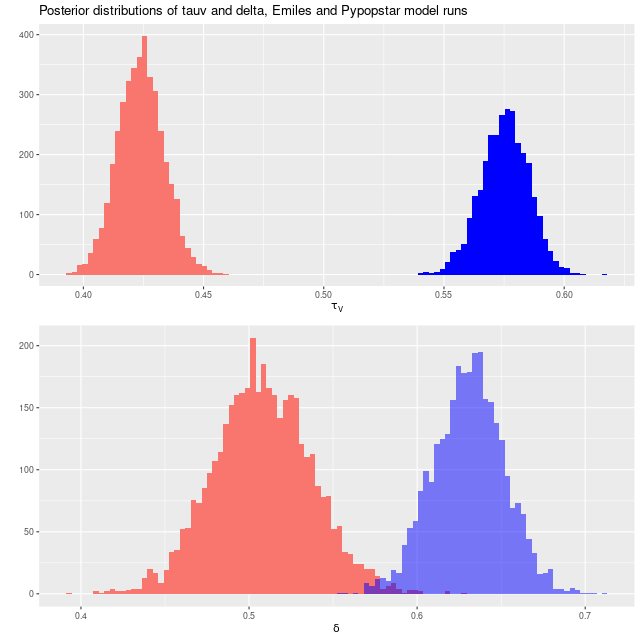
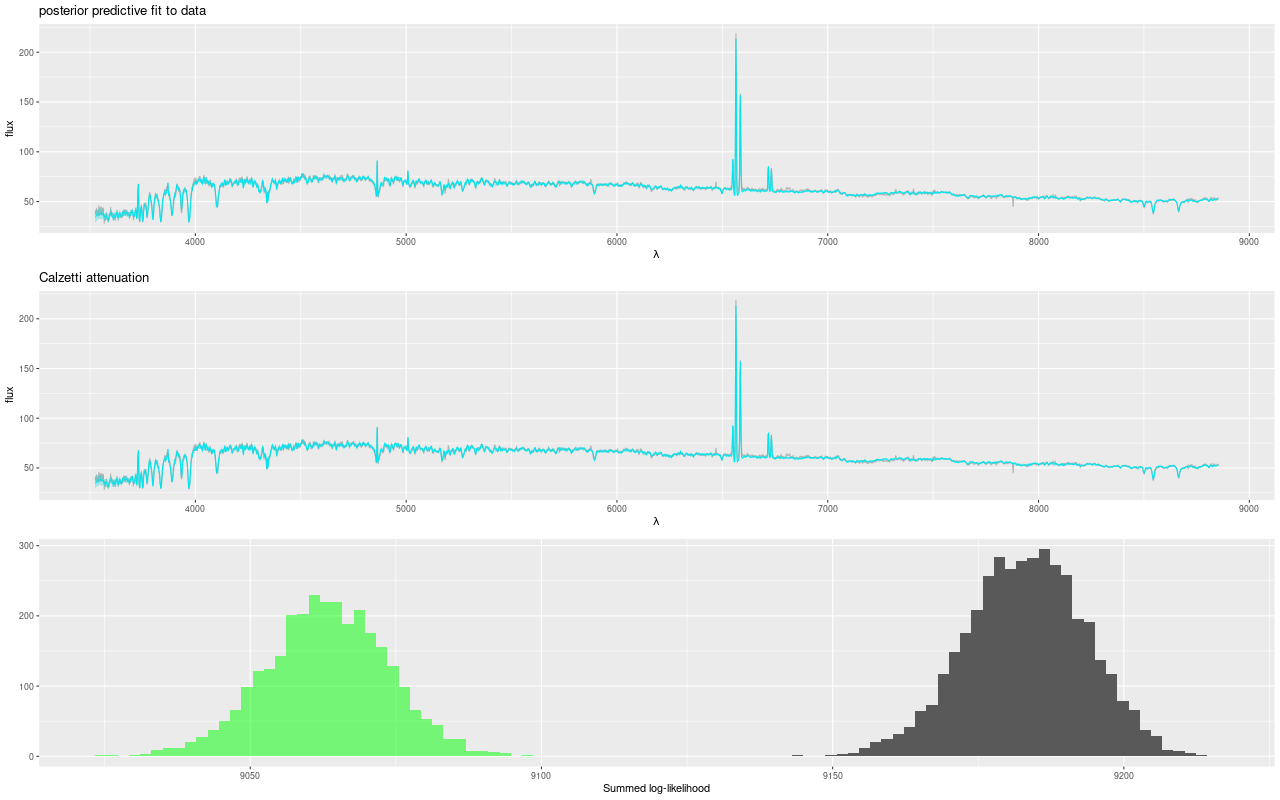
In the models I ran last year I ignored dust reddening since I didn’t expect it to be significant in the passively evolving Coma cluster galaxies I tested them on. In general reddening isn’t ignorable though and there’s the potential for template mismatch without some allowance for it. For now I inserted the function I use for “modified Calzetti” attenuation but it’s not actually used. In the one test I tried including attenuation in the model significantly increased execution time. I will probably look at using a multiplicative polynomial for the same purpose. A final thing to note is there are no explicit priors for the two simplex vectors that represent the stellar velocity convolution kernel and emission line profile, which means that the priors default to a maximally diffuse dirichlet distribution. This turns out to be an important issue that I will discuss further below.
I’ve run sets of models for a small sample of galaxies so far. so lets look at some results. For these runs I used 500 warmup and 500 post-warmup iterations per chain with 4 parallel chains for a total post-warmup sample size of 2000. The stellar templates are represented by 6 eigenspectra created from singular value decompositions of my standard EMILES based SSP library. I currently fit 18 emission lines — Balmer lines from Hα through Hζ and a selection of the stronger forbidden lines. Model runs typically take 2-3 minutes for sampling on my old 4th generation Intel core I7 based PC. This can undoubtedly be reduced by factors of at least several with multithreading.
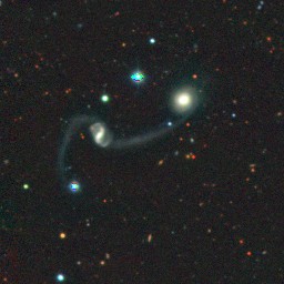
In this post I’m going to look in some detail at results for Markarian 888, which was the main topic of my last post. Recall this is one of Schawinski’s “blue early type galaxies” that turns out to have obvious spiral-like structure in its inner region and clear evidence for a relatively recent merger.
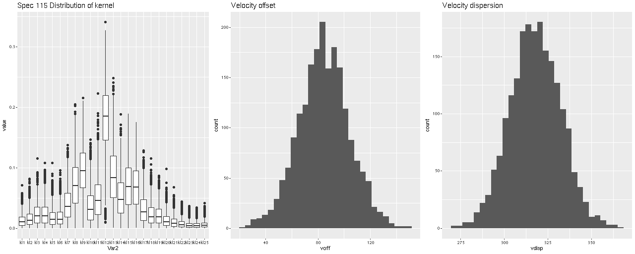
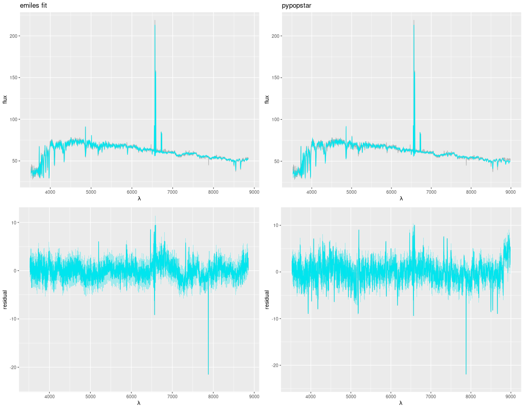
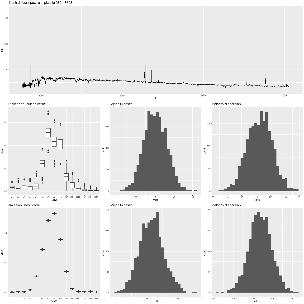
First, the graph below shows the central fiber spectrum, and below that the results of a model run for the stellar velocity convolution kernel. From those I can calculate velocity offsets1these formulas are approximate but close enough for the present purpose.
\( \delta v = 69 \times \sum\limits_{k = -\lfloor K/2 \rfloor}^{\lfloor K/2 \rfloor} k p_i \)and velocity dispersions
\(v_{disp} = 69 \times \sqrt{\sum\limits_{k = -\lfloor K/2 \rfloor}^{\lfloor K/2 \rfloor} k^2 p_i – \delta v^2}
\)
for each draw from the posteriors, and these are shown as histograms in the middle and right graphs. This was a high signal to noise spectrum with prominent emission and absorption lines, a favorable situation for this modeling exercise and in fact the results look very promising with an especially well determined distribution for the emission lines. In summary, the posterior mean stellar velocity offset was 25 km/sec. with a 95% credible interval of (19.8, 31.3), while the corresponding values for emission lines were 24.3 and (22.8, 25.9), so the credible interval for emission lines lies entirely within that for stars.
The corresponding values for velocity dispersions on the other hand differ quite a lot: 141 km/sec. for stars with a 95% credible interval of (133.6, 150.3) versus 109 km/sec and (106, 111) for gas. I’ll say some more about this below, but I think this is already a sign that the second moments (at least) of these velocity distributions need to be treated with caution.
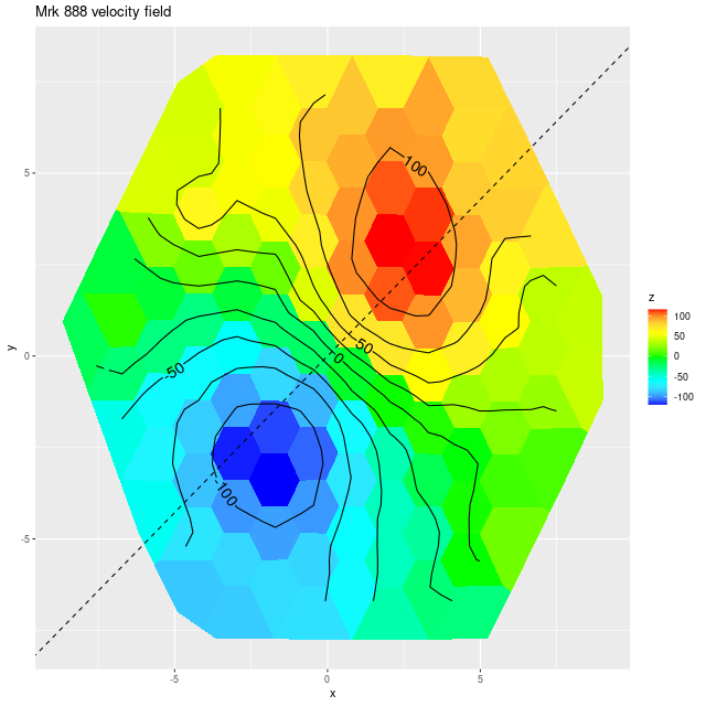
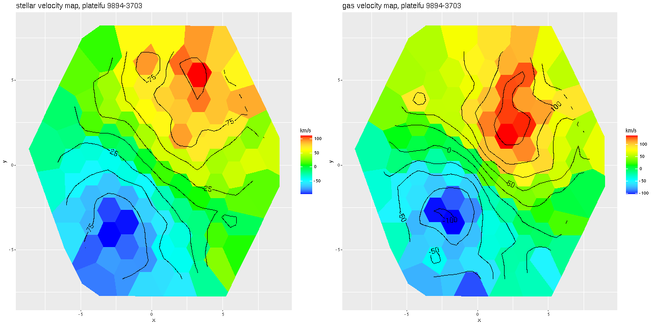
After running the code for every binned spectrum in the IFU I get stellar and gas velocity maps as shown below. These look similar to each other and to the map in the last post based on my hybrid red shift offset fitting routine, although a closer look will show a systematic decoupling of gas and stellar velocities.
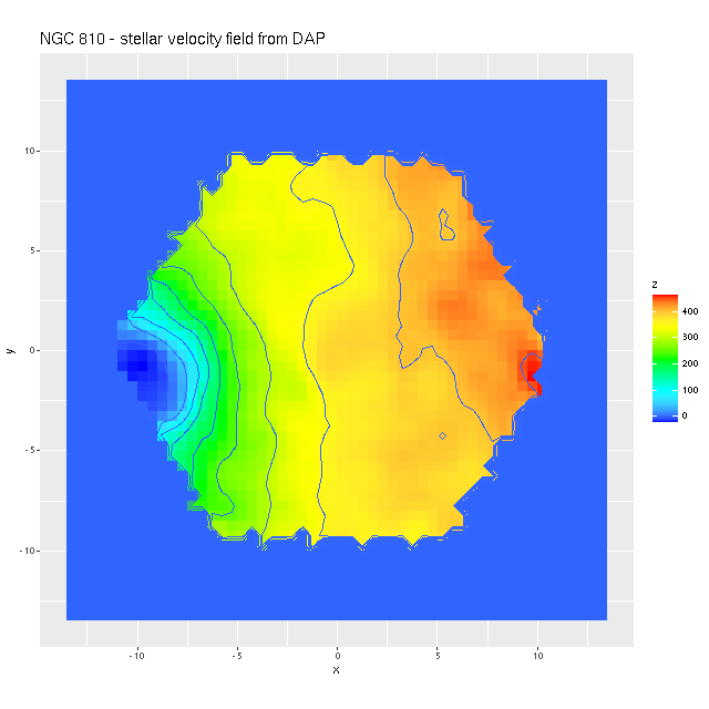
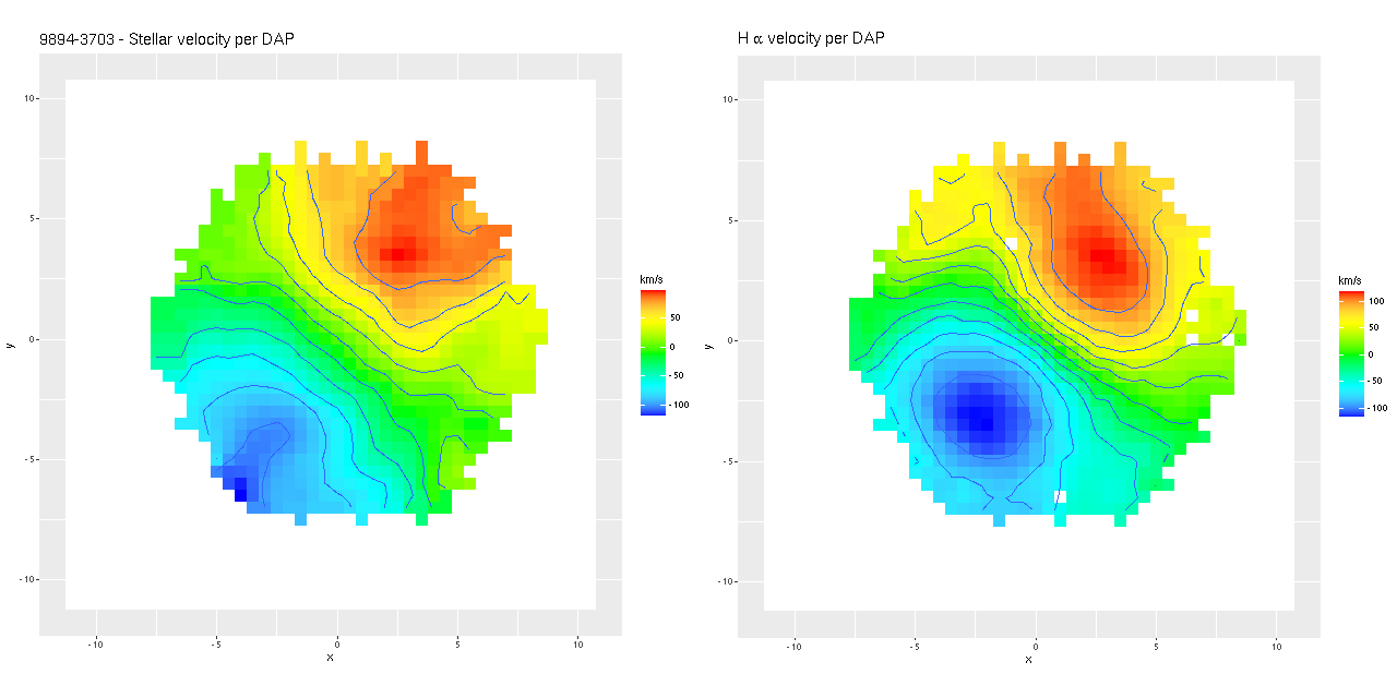
I often take a look at the official MaNGA data analysis pipeline results, usually through the “Marvin” interface. Generally my results look similar for any given quantity, but it’s hard to tell how closely since we’re looking at different things (binned RSS spectra vs. cubes, for one) and I’m really just doing a visual comparison. As more or less a one off exercise I decided to compare velocity fields from the cubes. First, here are stellar and Hα maps from the DAP. These are from the “HYB10-MILESHC-MASTARSSP” sequence, which refers to the binning strategy and template inputs.
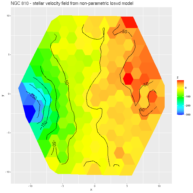
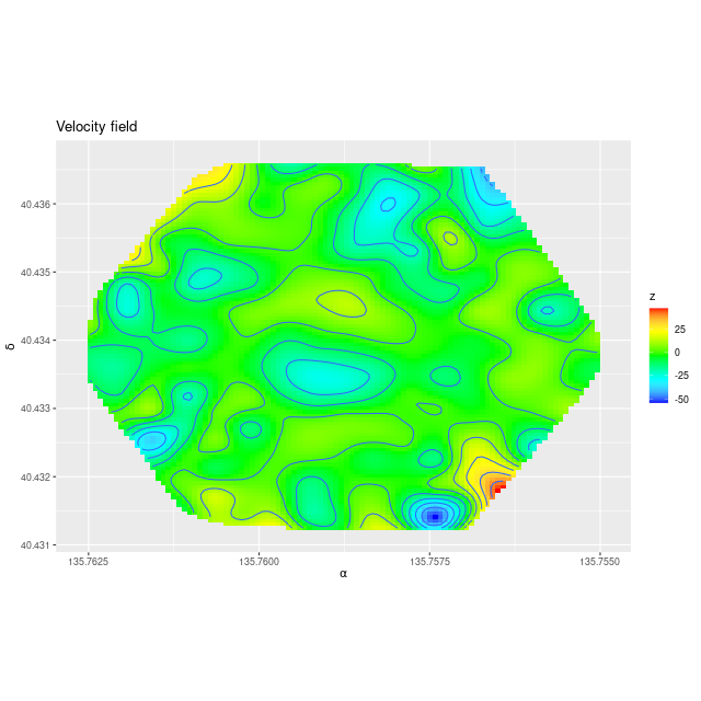
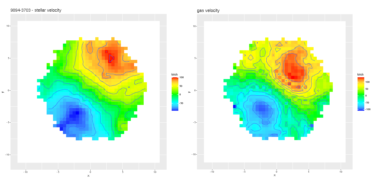
Next are my stellar and ionized gas velocity maps. Evidently these are considerably “noisier” in appearance, but similar overall. The noisiness may be due to different binning strategies: I modeled velocity distributions for every spaxel that met a minimal signal to noise requirement.
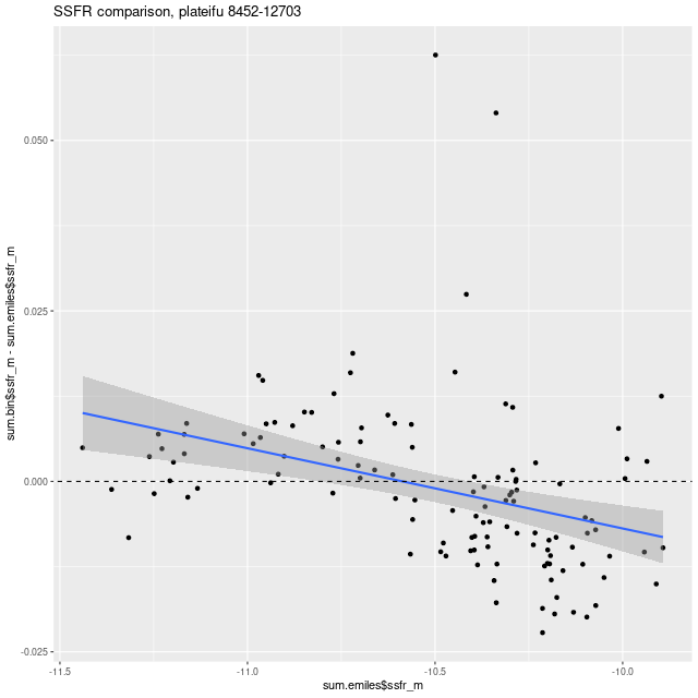
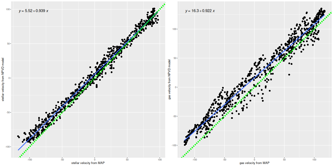
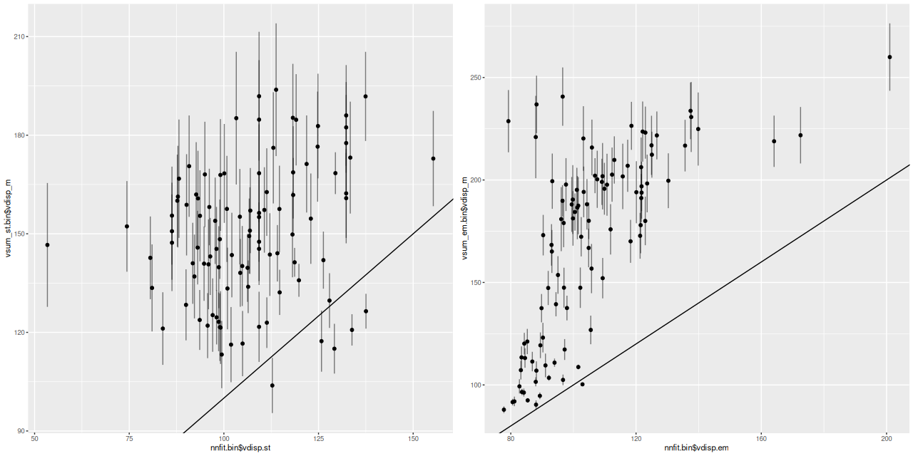
For a more quantitative comparison here are scatterplots of the mean stellar and gas velocity offsets from my runs against the MaNGA DAP. Both of these show slight tilts, that is the slopes are less than one, and small offsets. I’m tempted to suspect systematic errors somewhere, but I haven’t found any yet. And I have no hypothesis about the decidedly non-random behavior of the gas velocity plots. So there are still questions to be answered, but the magnitude of differences is no more than about ±1 wavelength bin (69 km/sec). For my main purposes this is good enough.
One more pair of graphs for this galaxy. In the initial maximum likelihood fit to a spectrum I estimate stellar and gas velocity dispersions with a single component gaussian. The graphs below plot the velocity dispersions from the Bayesian models calculated by the formula above against the ML fit values. The stellar velocity dispersions behave pretty much the same as I noted before: there’s a weak positive correlation between the non-parametric models and the maximum likelihood estimates with the former generally offset to higher values. The gas velocity dispersion estimates show an even larger discrepancy along with an apparently nonlinear trend.
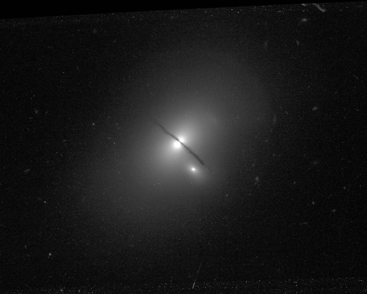
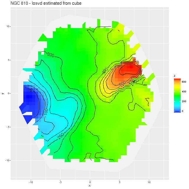
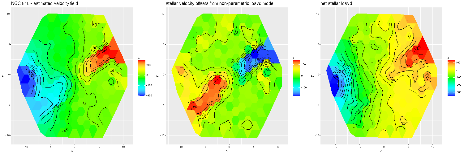
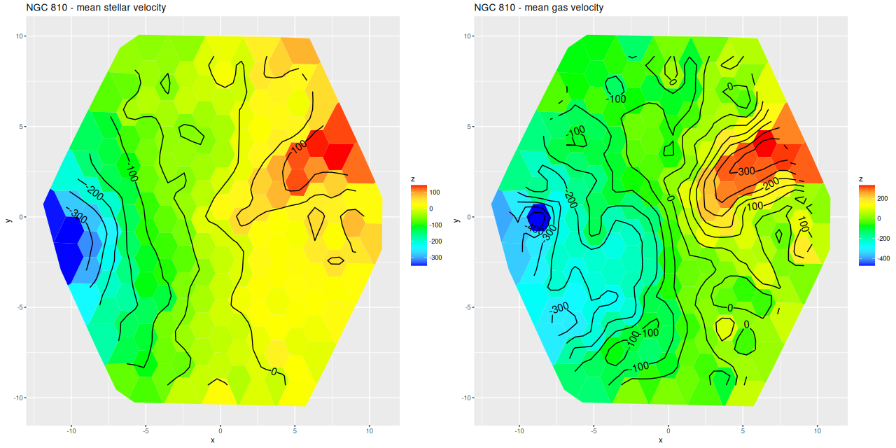
More briefly now, since this got longer than I wanted. I also ran models for the “Zoogems” target NGC 810, which I noted two posts ago has interesting kinematics, in particular a rapidly rotating disk that isn’t evident in the stellar velocity map from the DAP. From the maps below we see that the rapidly rotating component is the ionized gas, which has a mean rotation velocity as much as 150 km/sec larger than the stellar component.
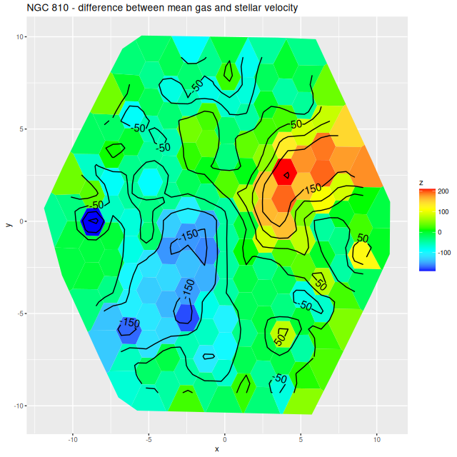
Finally, here are two more graphs of the kinematic models for the spectra with the largest positive and negative differences between stellar and gas velocity (these are the reddest and bluest patches in the map above. These show the spectra in the top row, followed by the posterior distribution of the stellar LOSVD and distributions of the first two moments, then the same for the emission line profiles.
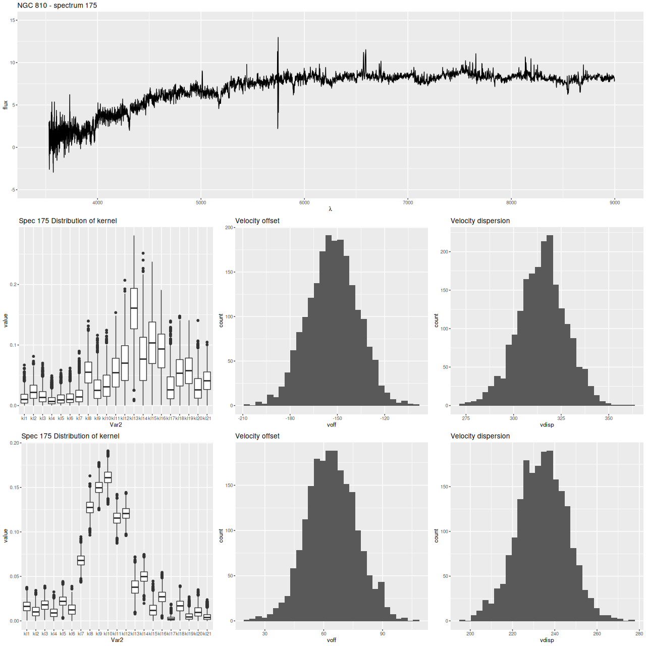
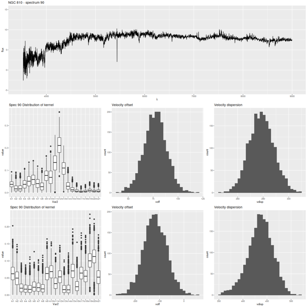
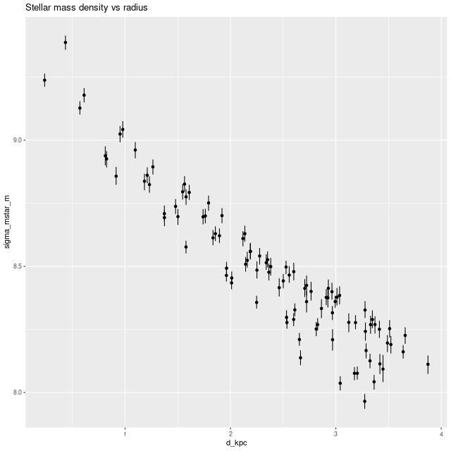
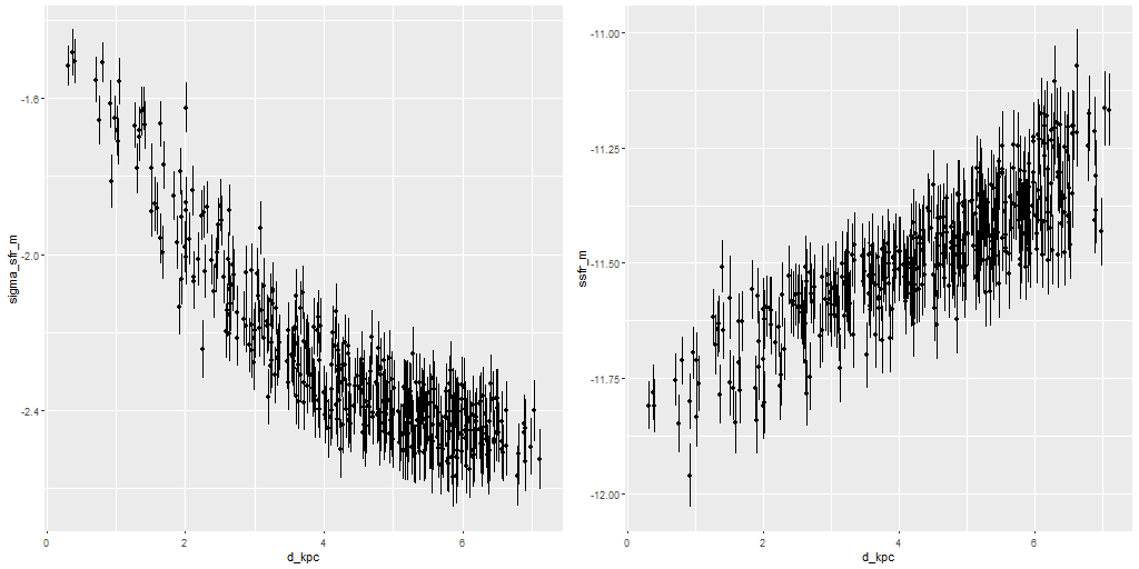
The second set of graphs illustrates a significant problem: when there’s poor data — in this case no detectable emission lines — the models tend to return the prior, which for now is a maximally diffuse dirichlet. This will bias second moment estimates to the high side and can lead to spurious correlations, for example the increase of velocity dispersion with radius that I noted in the last post on this topic.
At the same time this spectrum is in the region of overlap between the main galaxy and its companion, and two peaks in the stellar velocity distribution are clearly seen at about the right velocity offset (~340 km/sec).
A short to do list:
- Investigate informative priors.
- Allow for dust reddening. I tried using a modified Calzetti attenuation relation in the code (note its presence in the code below, although it’s not used in the model), but it adds too much to execution time. A low order multiplicative polynomial might suffice.
- Investigate systematics between my estimates and those in the DAP.