
It’s been available for a while actually, but not in a form I’ve been able to figure out how to use. That changed recently with the introduction of the reduce_sum “higher order function” in Stan 2.23.0. What reduce_sum does is allow data to be partitioned into conditionally independent slices that can be dispatched to parallel threads if the Stan program is compiled with threading enabled. My SFH modeling code turns out to be an ideal candidate for parallelization with this technique since flux errors given model coefficients and predictor values are treated as independent1This is an oversimplification since there is certainly some covariance between nearby wavelength bins. This is rarely if ever modeled though and I haven’t figured out how to do it. In any case adding covariance between measurements would complicate matters but not necessarily make it impossible to partition into independent chunks. Here is the line of Stan code that defines the log-likelihood for the current version of my model (see my last post for the complete listing):
    gflux ~ normal(a * (sp_st*b_st_s) .* calzetti_mod(lambda, tauv, delta)
                    + sp_em*b_em, g_std);
This just says the galaxy flux values are drawn from independent gaussians with mean given by the model and known standard deviations. Modifying the code for reduce_sum requires a function to compute a partial sum over any subset of the data for, in this case, the log-likelihood. The partial sum function has to have a specific but fairly flexible function signature. One thing that confused me initially is that the first argument to the partial sum function is a variable to be sliced over that, according to the documentation, must be an array of any type. What was confusing was that passing a variable of vector type as the first argument will fail to compile. In other words a declaration in the data block like
vector[N] y;
with, in the functions block:
real partial_sum(vector y, ...);
fails, while
real y[N];

real partial_sum(real[] y, ...);
works. The problem here is that all of the non-scalar model parameters and data are declared as vector and matrix types because the model involves vector and matrix operations that are more efficiently implemented with high level matrix expressions. Making gflux the sliced variable, which seemed the most obvious candidate, won’t work unless it’s declared as real[] and that won’t work in the sampling statement unless it is cast to a vector since the mean in the expression at the top of the post is a vector. Preliminary investigation with a simpler model indicated that approach works but is so slow that it’s not worth the effort. But, based on a suggestion in the Stan discussion forum a simple trick solved the issue: declare a dummy variable with an array type, pass it as the first argument to the partial sum function, and just don’t use it. So now the partial sum function, which is defined in the functions block is
  real sum_ll(int[] ind, int start, int end, matrix sp_st, matrix sp_em,
              vector gflux, vector g_std, vector lambda, real a, real tauv, real delta,
              vector b_st_s, vector b_em) {
    return normal_lpdf(gflux[start:end] | a * (sp_st[start:end, :]*b_st_s) .* calzetti_mod(lambda[start:end], tauv, delta)
                    + sp_em[start:end, :]*b_em, g_std[start:end]);
  }
I chose to declare the dummy variable ind in a transformed data block. I also declare a tuning variable grainsize there and set it to 1, which tells Stan to set the slice size automatically at run time.
transformed data {
  int grainsize = 1;
  int ind[nl] = rep_array(1, nl);
}
Then the sampling statement in the model block is
    target += reduce_sum(sum_ll, ind, grainsize, sp_st, sp_em, gflux, g_std, lambda,
                          a, tauv, delta, b_st_s, b_em);
The rest of the Stan code is the same as presented in the last post.
So why go to this much trouble? As it happens a couple years ago I built a new PC with what was at the time Intel’s second most powerful consumer level CPU, the I9-7960X, which has 16 physical cores and supports 32 threads. I’ve also installed 64GB of DRAM (recently upgraded from 32), which is overkill for most applications but great for running Stan programs which can be rather memory intensive. Besides managing my photo collection I use it for Stan models, but until now I haven’t really been able to make use of its full power. By default Stan runs 4 chains for MCMC sampling, and these can be run in parallel if at least 4 cores are available. It would certainly be possible to run more than 4 chains but this doesn’t buy much: increasing the effective sample size by a factor of 2 or even 4 doesn’t really improve the precision of posterior inferences enough to matter. Once I tried running 16 chains in parallel with a proportionate reduction in post-warmup iterations, but that turned out to be much slower than just using 4 chains. The introduction of reduce_sum raised at least the possibility of making full use of my CPU, and in fact working through the minimal example in Stan’s library of case studies indicated that close to factor of 4 speedups with 4 chains and 4 threads per chain are achievable. I got almost no further improvement setting the threads per chain to 8 and thus using all virtual cores, which apparently is expected at least with Intel CPUs. I haven’t yet tried other combinations, but using all physical cores with the default 4 chains seems likely to be close to optimal. I also haven’t experimented much with the single available tuning parameter, the grainsize. Setting it equal to the sample size divided by 4 and therefore presumably giving each thread an equal size slice did not work better than letting the system set it, in fact it was rather worse IIRC.
I’ve run both the threaded and unthreaded models on one complete set of data for one MaNGA galaxy. This particular data set used the smallest, 19 fiber IFU, which produces 57 spectra in the stacked RSS data. This was binned to 55 spectra, all with SNR > 5. The galaxy is a passively evolving S0 in or near the Coma cluster, but I’m not going to discuss its star formation history in any detail here. I’m only interested in comparative runtimes and the reproducibility of sampling. And here is the main result of interest, the runtimes (for sampling only) of the threaded and unthreaded code. All runs used 4 chains with 250 warmup iterations and 750 post-warmup. I’ve found 250 warmup iterations to be sufficient almost always and 3000 total samples is more than enough for my purposes. This is actually an increase from what had been my standard practice.
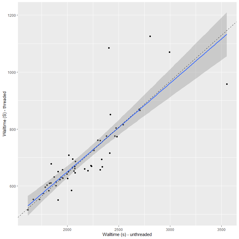
On average the threaded code ran a factor of 3.1 times faster than the unthreaded, and was never worse than about a factor 2 faster2but also never better than a factor 3.7 faster. This is in line with expectations. There’s some overhead involved in threading so speedups are rarely proportional to the number of threads. This is also what I found with the published minimal example and with a just slightly beyond minimal multiple regression model with lots of (fake) data I experimented with. I’ve also found the execution time for these models, particularly in the adaptation phase, to be highly variable with some chains occasionally much faster or slower than others. Stan’s developers are apparently working on communicating between chains during the warmup iterations (they currently do not) and this might reduce between chain disparities in execution time in the future.
I’m mostly interested in model star formation histories, so here’s the comparison of star formation rate densities for both sets of model runs on all 55 bins, ordered by distance from the IFU center (which coincides with the galaxy nucleus):
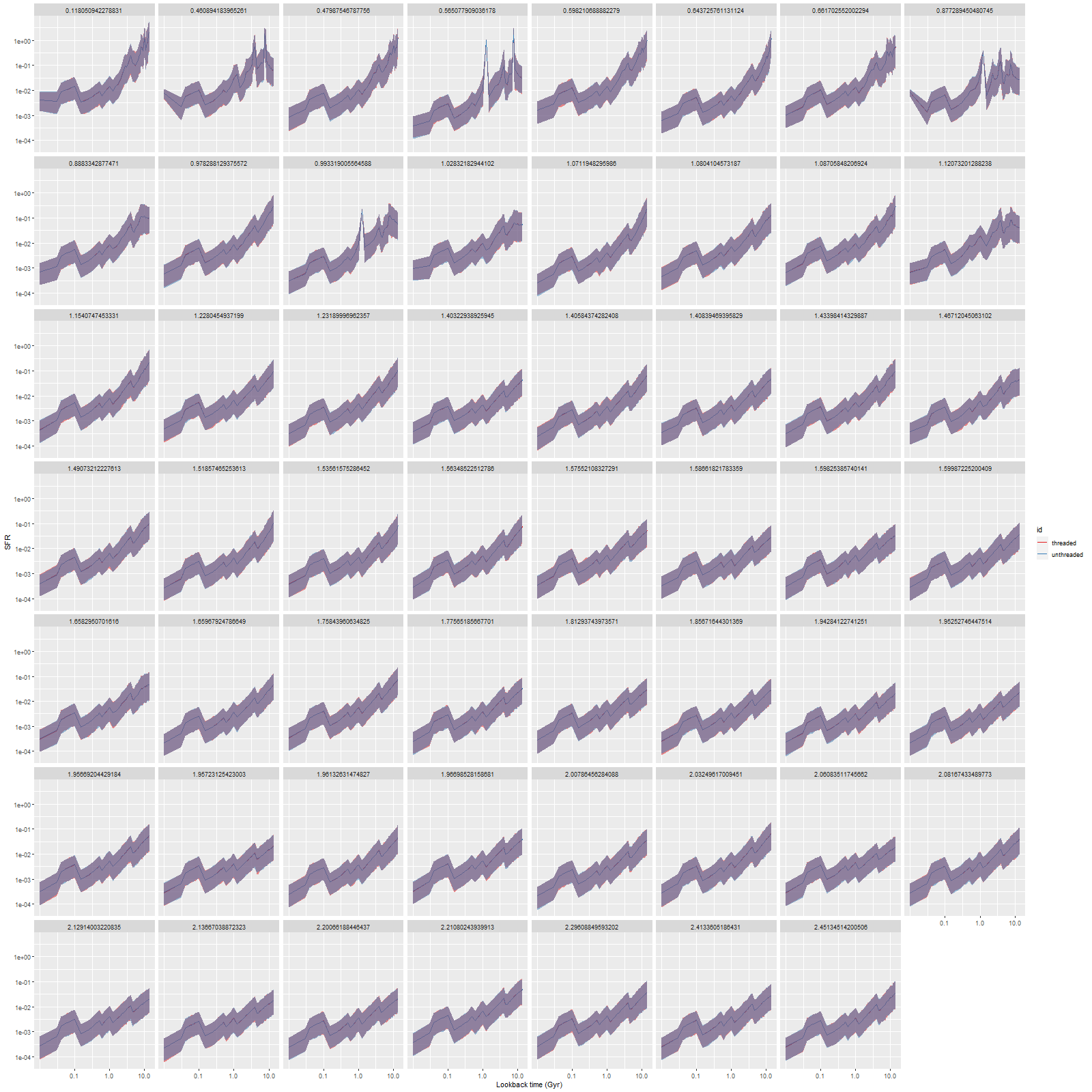
Notice that all the ribbons are purple (red + blue), indicating the two sets of runs were nearly enough identical. Exact reproducibility is apparently hard to achieve in multithreaded code, and I didn’t try. I only care about reproducibility within expected Monte Carlo variations, and that was clearly achieved here.
There are only a few down sides to multithreading. The main one is that rstan is currently several dot releases behind Stan itself and seems unlikely to catch up to 2.23.x before 2021. I do extensive pre- and post-processing in R and all of my visualization tools use ggplot2 (an R package) and various extensions. At present the best way to integrate R with a current release of Stan is a (so far) pre-release package called cmdstanr, which bills itself as a “lightweight interface to Stan for R users.” What it actually is is an interface between R and cmdstan, which is in turn the command line driven interface to Stan.
By following directions closely and with a few hints from various sources I was able to install cmdstan from source and with threading support in Windows 10 using Rtools 4.0. The development version of cmdstanr is trivial to install and seems to work exactly as advertised. It is not a drop in replacement for rstan though, and this required me to write some additional functions to fit it into my workflow. Fortunately there’s an rstan function that reads the output files from cmdstan and creates a stanfit object, and this enables me to use virtually all of my existing post-processing code intact.
The other consequence is that cmdstan uses R dump or json format files for input and outputs csv files, the inputs have to be created on the fly, and the outputs have to be read into memory. Cmdstanr with some help from rstan handles this automatically, but there’s some additional overhead compared to rstan which AFAIK keeps all data and sampler output in memory. On my machine the temporary directories reside on a SSD, so all this file I/O goes fairly quickly but still slower than in memory operations. I also worry a bit about the number of read-write cycles but so far the SSD is performing flawlessly.
Multithreading is beneficial to the extent that physical cores are available. This is great for people with access to HPC clusters and it’s helpful to me with an overspec’d and underutilized PC. My current Linux box, which is really better suited to this type of work, only has a several generations old Intel I7 with 4 cores. It’s still a competent and highly reliable machine, but it’s not likely to see any performance improvement from multithreading. Fortunately the current trend is to add more cores to mainstream CPUs: AMD’s Ryzen line currently tops out at 16 cores and their Threadripper series have 24-64 cores. This would be a tempting next build, but alas I’m trying not to spend a lot of money on hobbies these days for more or less obvious reasons.
Update 6/27/2020
Sampling time and total execution time
I got some uninterrupted model runs done on the two PC’s I’m currently using for these models remembering to measure the total execution time using system.time() and sampler time returned by rstan or cmdstan. These were for 3 galaxies apiece with 825 total spectra analyzed on the I9 based system and 150 on the I7 based. In slightly more detail the two systems are (1) an Intel I7-4790K CPU with 4 physical cores (8 threads) running at 4GHz, 32GB DDR3 RAM, SATA HDDs local storage running Fedora 32; and (2) Intel I9-7960X CPU (16 cores, 32 threads), 64GB DDR4 RAM, SATA HDD and SSD local storage running Windows 10 Pro. Both machines are running R 4.0.0. The current version of rstan is 2.19.3 and StanHeaders is 2.19.2. The I9 based timings used cmdstan 2.23.0 run in R through cmdstanr 0.0.9000 with 4 chains and 4 threads per chain. The Linux machine uses gcc 10.1.1 while on Windows I use the Rtools 4.0 toolset with mingw 64 bit compiler. Here’s a brief summary of average times per spectrum. All runs used 250 warmup and 750 post-warmup iterations for 4 chains. The adaptation parameters were set to max_treedepth = 11 and adapt_delta = 0.9.
| Total time (S) | Sampling time | Difference | |
| I7 | 3664 | 3555 | 108 |
| I9 | 933 | 762 | 171 |
| ratio | 3.92 | 4.66 | 0.63 |
The overhead, that is the difference between the total execution time and time spent in the sampler, results from several pre- and post processing steps. I use the maximum likelihood solutions from the non-negative least squares fits as inputs to Stan’s optimizer to estimate MAP fits. These are then used with some added random jitter to initialize parameter values for sampling. After sampling I do some basic checkpointing: sampled values for model parameters are retrieved from the stanfit objects and saved to a file. The overhead is rather worse for the I9 runs, by 63 seconds per model run. This is the minimum penalty for the extra file I/O involved in passing data to and from cmdstan. The nearly factor of 5 improvement in sampling time reflects the improvement due to multi-threading and increased performance from the later generation Intel processor. Investing in new hardware is really tempting!
Threading
Here’s a quick graphical summary of varying the number of threads per chain used by the sampler. This CPU has 16 physical cores and up to 32 threads. These timings are for a single MaNGA spectrum, with 4 chains run in parallel and the same number of iterations and adaptation parameters as before. I did not set the random number seed for any run, so this produces a little extra variability in times.
The graph shows the ratio of the single threaded execution time to the multi-threaded time. This ratio is plotted for each chain — of course the total time is determined by the slowest chain and these are connected by lines.
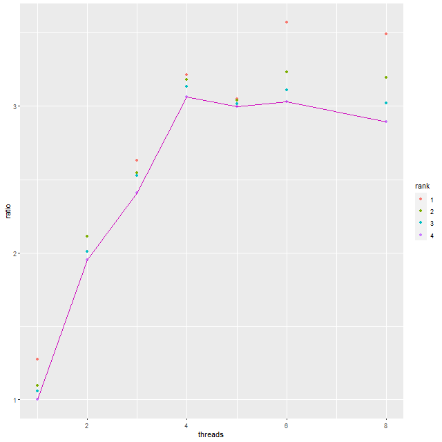
Not much of a surprise here: threading improves performance up until the number of chains times the number of threads equals the number of physical cores. Above that there’s no further improvement or even a small penalty in performance.