I only have time to analyze one MaNGA galaxy for now and since it was the first to get the correctly coded LOSVD estimates I chose the Coma Cluster S0 galaxy NGC 4949 that I discussed in the last post for SFH modeling. As I mentioned a few posts ago trying to model the LOSVD and star formation history simultaneously is far too computationally intensive for my resources, so for now I just convolve the SSP model spectral templates with the elementwise means of the convolution kernels estimated as described previously and feed those to the SFH modeling code. My intuition is that the SFH estimates should be at least slightly more variable if the kinematics are treated as variable as well, but for now there’s no real alternative to just picking a fiducial value. Of course a limited test of that hypothesis could be made by pulling multiple draws from the posterior of the LOSVD distribution. I will certainly try that in the future.
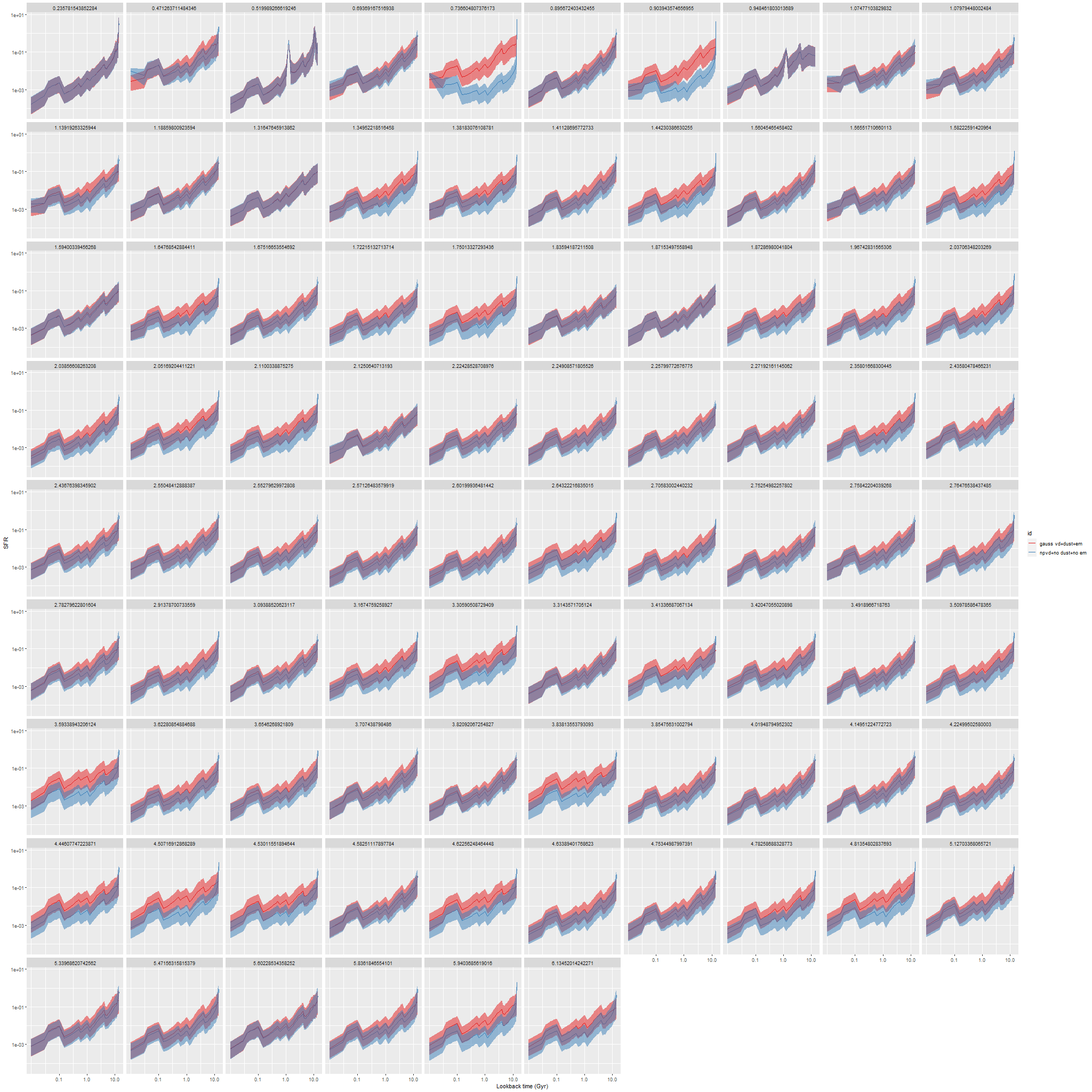
My first idea was to leave both dust and emission lines out of the SFH models. The first choice was to save CPU cycles and also based on the expectation that these passively evolving galaxies should have very little dust. The results were rather interesting: here are ribbon plots of model SFH’s for all 86 binned spectra. The pink ribbons are from the original model runs, which assumed single component gaussian velocity distributions, modified Calzetti attenuation, and included emission lines (which contribute negligible flux throughout). The blue ribbons are with non-parametric LOSVD and no attenuation model:
NGC 4949 – modeled star formation histories with single component gaussian and nonparametric estimates of line of sight velocity distributions with no dust model
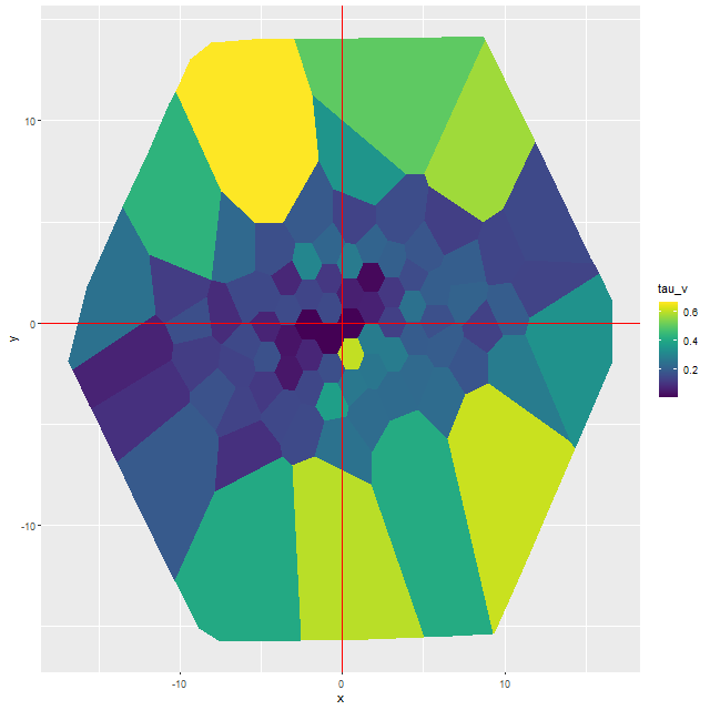
The differences in star formation histories turn out to be almost entirely due to neglecting dust in the second set of model runs. In this galaxy there are some areas with apparently non-negligible amounts of dust:
NGC 4949 – map of estimated optical depth of attenuation
Ignoring attenuation forces the model to use redder, hence older (and probably more metal rich although I haven’t yet checked) stellar populations and this has, in some cases, profound effects on the model SFH.
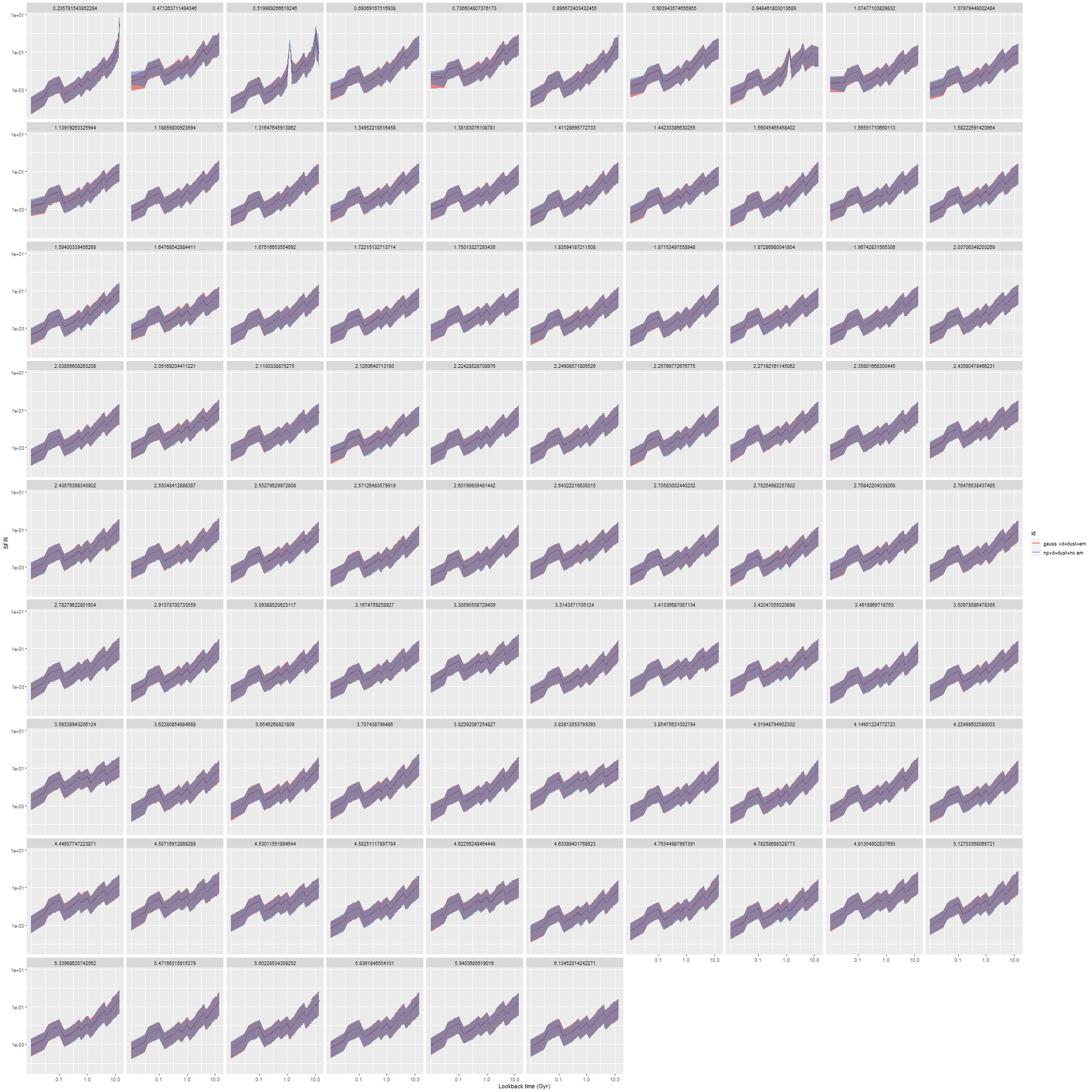
So, I tried a second set of model runs adding back in modified Calzetti attenuation but still leaving out emission:
NGC 4949 – modeled star formation histories with single component gaussian and nonparametric estimates of line of sight velocity distributions
And now the models are nearly identical, with minor differences mostly in the youngest age bin. All other quantities that I track are similarly nearly identical in both model runs.
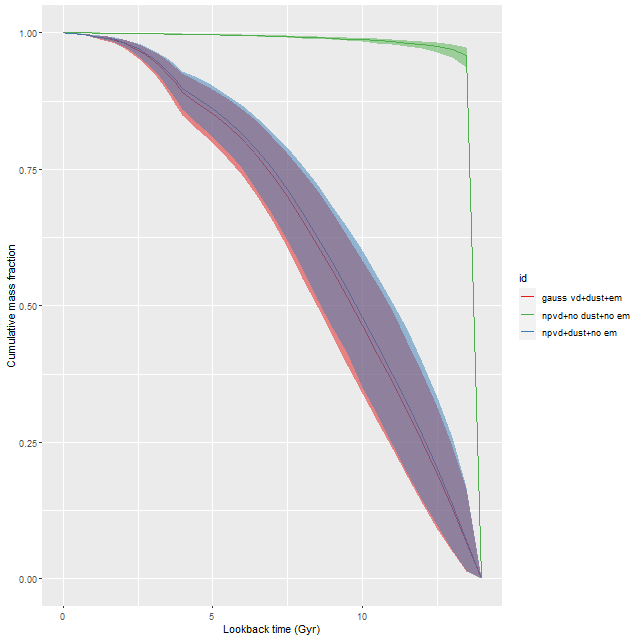
Here is the modeled mass growth history for a single spectrum of a region just south of the nucleus that had the largest difference in model SFH in the second set of runs, and the largest optical depth of attenuation in the first and 3rd. This is an extreme case of the shift towards older populations required by the neglect of reddening. Well over 90% of the present day stellar mass was, according to the model, formed in the first half Gyr after the big bang with almost immediate and complete quenching thereafter. While not an impossible star formation history it’s not one I often see result from these models, which strongly favor more gradual mass buildup.
NGC 4949 – modeled mass growth histories for models with and without an attenuation model
So, the conclusion for now is that having an attenuation model matters a lot, the detailed stellar kinematics not so much. Of course this is a relatively simple example because it’s a rapid rotator and the model convolution kernels are fairly symmetrical throughout the galaxy. The massive ellipticals and especially cD galaxies with more complex kinematics might provide some surprises.
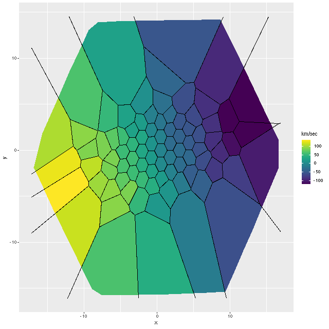
Well that was simple enough. I made a simple indexing error in the R data preprocessing code that resulted in a one pixel offset between the template and galaxy spectra, which effectively resulted in shifting the elements of the convolution kernel by one bin. I had wanted to look at a rotating galaxy to perform some diagnostic tests, but once I figured out my error this turned out to be a pretty good validation exercise. So I decided to make a new post. The galaxy I’m looking at is NGC 4949, another member of the sample of passively evolving Coma cluster galaxies of Smith et al. It appears to me to be an S0 and is a rapid rotator:
NGC 4949 – SDSS imageNGC 4949 – radial velocity map
These projected velocities are computed as part of my normal workflow. I may in a future post explain in more detail how they’re derived, but basically they are calculated by finding the best redshift offset from the system redshift (taken from the NSA catalog which is usually the SDSS spectroscopic redshift) to match the features of a linear combination of empirically derived eigenspectra to the given galaxy spectrum.
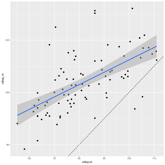
First exercise: find the line of sight velocity distribution after adjusting to the rest frame in each spectrum. This was the originally intended use of these models. This galaxy has fairly low velocity dispersion of ~100 km/sec. so I used a convolution kernel size of just 11 elements with 6 eigenspectra in each fit. Here is a summary of the LOSVD distribution for the central spectrum. This is much better. The kernel estimates are symmetrical and peak on average at the central element. The mean velocity offset is ≈ 9.5 km/sec, which is much closer to 0 than in the previous runs. I will look briefly at velocity dispersions at the end of the post: this one is actually quite close to the one I estimate with a single component gaussian fit (116 km/sec vs 110).
Estimated LOSVD of central spectrum of NGC 4949
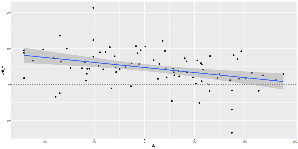
Next, here are the posterior mean velocity offsets for all 86 spectra in the Voronoi binned data, plotted against the peculiar velocity calculated as outlined above. The overall average of the mean velocity offsets is 4.6 km/sec. The reason for the apparent tilt in the relationship still needs investigation.
Mean velocity offset vs. peculiar velocity. All NGC 4949 spectra.
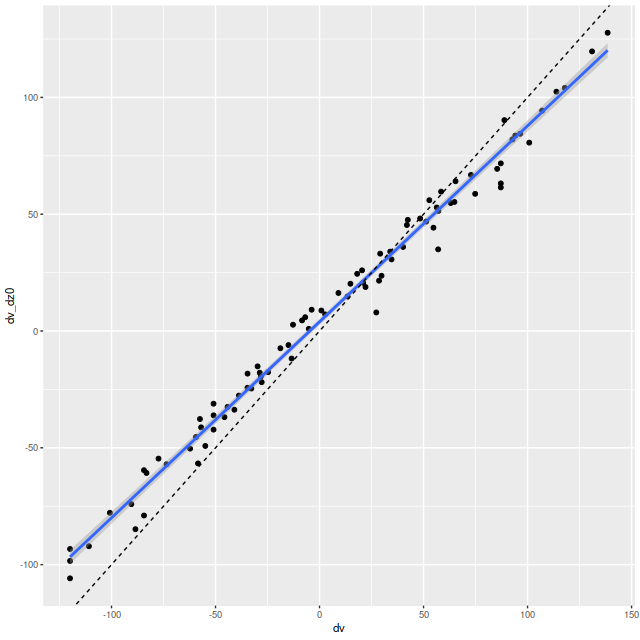
Exercise 2: calculate the LOSVD with wavelengths adjusted to the overall system redshift as taken from the NSA catalog, that is no adjustment is made for peculiar redshifts due to rotation. For this exercise I increased the kernel size to 17 elements. This is actually a little more than needed since the projected rotation velocities range over ≈ ± 100 km/sec. First, here is the radial velocity map:
Radial velocity map from Bayesian LOSVD model with no peculiar redshifts assigned.
Here’s a scatterplot of the velocity offsets against peculiar velocities from my normal workflow. Again there’s a slight tilt away from a slope of 1 evident. The residual standard error around the simple regression line is 6.4 km/sec and the intercept is 4 km/sec, which are consistent with the results from the first set of LOSVD models.
Velocity offsets from Bayesian LOSVD models vs. peculiar velocities
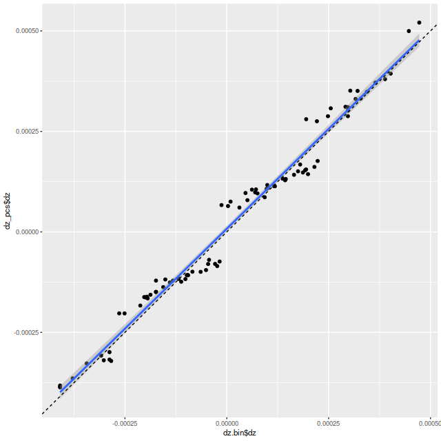
Exercise 3: calculate redshift offsets using a set of (for this exercise, 6) eigenspectra from the SSP templates. Here is a scatterplot of the results plotted against the redshift offsets from my usual empirically derived eigenspectra. Why the odd little jumps? I’m not completely sure, but my current code does an initial grid search to try to isolate the global maximum likelihood, which is then found with a general purpose nonlinear minimizer. The default grid size is 10-4, about the size of the gaps. Perhaps it’s time to revisit my search strategy.
Redshift offsets from a set of SSP derived eigenspectra vs. the same routine using my usual set of empirically derived eigenspectra.
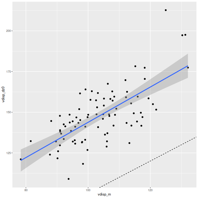
Final topic for now: I mentioned in the last post that posterior velocity dispersions (measured by the standard deviation of the LOSVD) were only weakly correlated with the stellar velocity dispersions that I calculate as part of my standard workflow. With the correction to my code the correlation while still weak has greatly improved, but the dispersions are generally higher:
Velocity dispersion form Bayesian LOSVD models vs. stellar velocity dispersion from maximum likelihood fits.
A similar trend is seen when I plot the velocity dispersions from the LOSVD models with correction only for the system redshift and a wider convolution kernel (exercise 2 above) with the fully corrected model runs (exercise 1):
These results hint that the diffuse prior on the convolution kernel is responsible for the different results. As part of the maximum likelihood fitting process I estimate the standard deviation of the stellar velocity distribution assuming it to be a single component gaussian. While the distribution of kernel values in the first graph look pretty symmetrical the tails are on average heavier than a gaussian. This can be seen too in the LOSVD models with the larger convolution kernel of exercise 2. The tails have non-negligible values all the way out to the ends:
Now, what I’m really interested in are model star formation histories. I’ve been using pre-convolved SSP model templates from the beginning along with phony emission line spectra with gaussian profiles with some apparent success. My plan right now is to continue that program with these non-parametric LOSVD’s. The convolutions could be carried out with posterior means of the kernel values or by drawing samples. Repeated runs could be used to estimate how much variation is affected by uncertainty in the kernel.
How to handle emission lines is another problem. For now stepping back to a simpler model (no emission, no dust) would be reasonable for this Coma sample.
This paper by J. Falcón-Barroso and M. Martig that showed up on arxiv back in November interested me for a couple reasons. First, this was one of the first research papers I’ve seen to make use of the Stan language or indeed any implementation of Hamiltonian Monte Carlo. What was even more interesting was they were doing exactly something I experimented with a few years ago, namely estimating the elements of convolution kernels for non-parametric description of galaxy stellar kinematics. And in fact their Stan code posted on github has comment lines linking to a thread on discourse.mc-stan.org I initiated where I asked about doing discrete convolution by direct multiplication and summation.
The idea I was pursuing at the time was to use sets of eigenspectra from a principal components decomposition of SSP model spectra as the bases for fitting convolved model spectra, with the expectation being that considerable dimensionality reduction could be achieved by using just the leading PC’s, which would in turn speed up model fitting. In fact this was certainly the case, although at the time I perhaps overestimated the number of components needed 1I mentioned in that thread that by one criterion — now forgotten — I would need 42, which is about an 80% reduction from the 216 spectra in the EMILES subset I use but still more than I expected. and I found the execution time to be disappointingly large. Another thing I had in mind was that I wanted to constrain emission line kinematics as well, and I couldn’t quite see how to do that in the same modeling framework. So, I soon turned away from this approach and instead tried to constrain both kinematics and star formation histories using the full SSP library and what I dubbed a partially parametric approach to kinematic modeling, using a convolution kernel for the stellar component and Gauss-Hermite polynomials for emission lines. This works, more or less, but it’s prohibitively computationally intensive, taking an order of magnitude or more longer to run than the models with preconvolved spectral templates. Consequently I’ve run this model fewer than a handful of times and only on a small number of spectra with complicated kinematics.
Falcón-Barroso and Martig started with exactly the same idea that I was pursuing of radically reducing the dimensionality of input spectral templates through the use of principal components. They added a few refinements to their models. They include additive Legendre polynomials in their spectral fits, and they also “regularize” the convolution kernels with informative priors of various kinds. Adding polynomials is fairly common in the spectrum fitting industry, although I haven’t tried it myself. There is only a short segment in the red that is sometimes poorly fit with the EMILES library, and that would seem to be difficult to correct with low order polynomials. What does affect the continuum over the entire wavelength range and could potentially cause a severe template matching issue is dust reddening, and this would seem to be more suitable for correction with multiplicative polynomials or simply with the modified Calzetti relation that I’ve been using for some time.
I’m also a little ambivalent about regularizing the convolution kernel. I’m mostly interested in the kinematics for the sake of matching the effective SSP model spectral resolution to that of the spectra being modeled for star formation histores, and not so much in the kinematics as such.
I decided to take another look at my old code, which somewhat to my surprise I couldn’t find stored locally. Fortunately I had posted the complete code on that discourse.mc-stan thread, so I just copied it from there and made a few small modifications. I want to keep things simple for now, so I did not add any polynomial or attenuation corrections and I am not trying to model emission lines. I also didn’t incorporate priors to regularize the elements of the convolution kernel. Without an explicit prior there will be an implicit one of a maximally diffuse dirichlet. I happen to have a sample of MaNGA spectra that are well suited for a simple kinematic analysis — 33 Coma cluster galaxies from a sample of Smith, Lucey, and Carter (2012) that were selected to be passively evolving based on weak Hα emission, which virtually guarantees overall weak emission. Passively evolving early type galaxies also tend to be nearly dust free, making it reasonable not to model it.
I’ve already run SFH models for all of these galaxies, so for each spectrum in a galaxy I adjust the wavelengths to rest frame using the system redshift and redshift offsets that were calculated in the previous round. I then regrid the SSP library (as usual the 216 component EMILES subset) templates to the galaxy rest frame and extract the region where there is coverage of both the galaxy spectrum and the templates. I then standardize the spectra (that is subtract the means and divide by the standard deviations) and calculate the principal components using R’s svd() function. I again rescale the eigenvectors to unit variance and select the number I want to use in the models. I initially did this by choosing a threshold for the cumulative sum of the eigenvalues as a fraction of the sum of all. I think instead I should use the square of the eigenvalues since that will make the choice based on the fraction of variance in the selected eigenvectors. With the former criterion a threshold of 0.95 will result in selecting 8 eigenspectra, 0.975 results in 13 (perhaps ± 1). In fact as few as 2 or 3 might be adequate as noted by Falcón-Barroso and Martig. The picture below of three eigenspectra from one model run illustrates why. The first two look remarkably like real galaxy spectra, with the first looking like that of an old passively evolving population, while the second has very prominent Balmer absorption lines and a bluer continuum characteristic of a younger population. After that the eigenspectra become increasingly un-spectrum like, although familiar features are still recognizable but often with sign flips.
First three eigenspectra from a principal components decomposition of an SSP model spectrum library
The number of elements in the convolution kernel is also chosen at run time. With logarithmic wavelength binning each wavelength bin has constant velocity width — for SDSS and MaNGA spectra of 69.1 km/sec. If a typical galaxy has velocity dispersion around 150 km/sec. and we want the kernel to be ≈ ±3 σ wide then we need 13 elements, which I chose as the default. Keep in mind that I’ve already estimated redshift offsets from the system value for each spectrum, so a priori I expected the mean velocity to be near 0. If peculiar velocities have to be estimated the convolution kernel would need to be much larger. Also in giant ellipticals and other fairly rare cases the velocity dispersion could be much larger as we’ll see below.
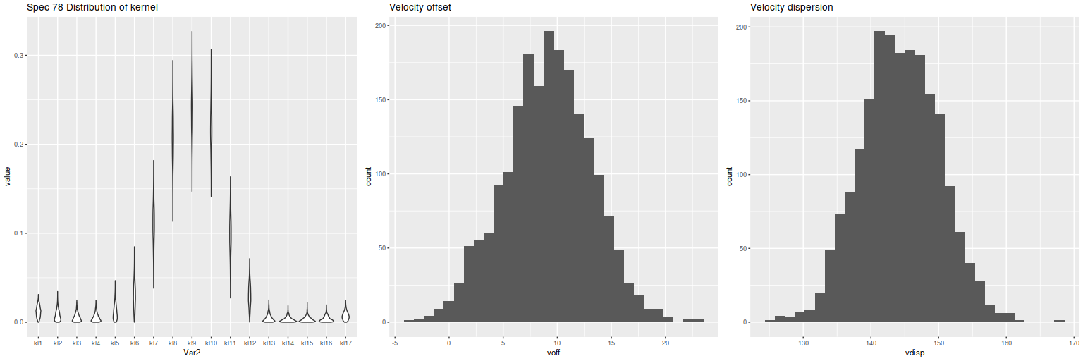
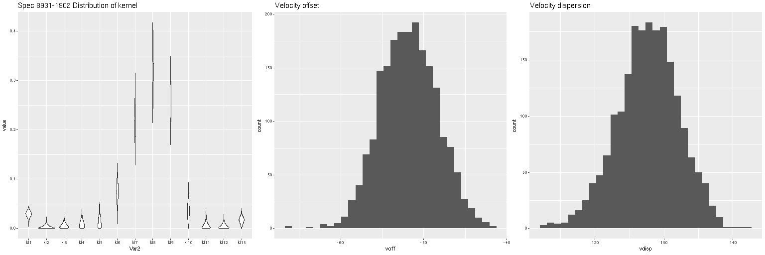
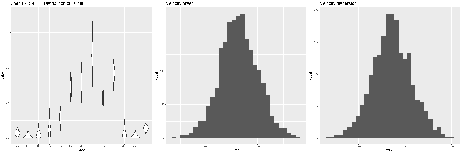
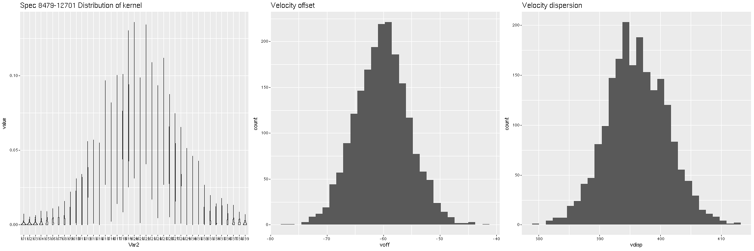
Lets look at a few examples. I’ve only run models so far for three galaxies with a total of 434 spectra. One of these (SDSS J125643.51+270205.1) appears disky and is a rapid rotator. The most interesting kinematically is NGC 4889, a cD galaxy at the center of the cluster. The third is SDSS J125831.59+274024.5, a fairly typical elliptical and slow rotator. These plots contain 3 panels. The left shows the marginal posterior distribution of the convolution kernels, displayed as “violin” plots. The second and third are histograms of the mean and standard deviation of the velocities. For now I’m just going to show results for the central spectrum in each galaxy. These are fairly representative although the distributions in each velocity bin get more diffuse farther out as the signal/noise of the spectra decrease. I set the kernel size to the default for the two lower mass galaxies. The cD has much higher velocity dispersion of as much as ~450 km/sec within the area of the IFU, so I selected a kernel size of 39 (± 1320 km/sec) for those model runs. The kernel appears to be fairly symmetrical for the rotating galaxy (top panes), while the two ellipticals show some evidence of multiple kinematic components. Whether these are real or statistical noise remains to be seen.
Distribution of kernel, velocity offset, and velocity dispersion. Central spectrum of MaNGA plateifu 8931-1902Distribution of kernel, velocity offset, and velocity dispersion. Central spectrum of MaNGA plateifu 8933-6101Distribution of kernel, velocity offset, and velocity dispersion. Central MaNGA spectrum of NGC 4889 (plateifu 8479-12701)
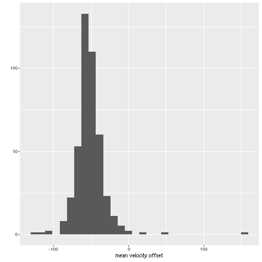
There are a couple surprises: the velocity dispersions summarized as the standard deviations of the weighted velocities are at best weakly correlated and generally larger than the values estimated in the preliminary fits that I perform as part of the SFH modeling process. More concerning perhaps is the mean velocity offset averages around -50 km/sec. This is fairly consistent across all three galaxies examined so far. Although this is less than one wavelength bin it is larger than the estimated uncertainties and therefore needs explanation.
Distribution of mean velocity offsets from estimated redshifts for 434 spectra in 3 MaNGA galaxies.
Some tasks ahead: Figure out this systematic. Look at regularization of the kernel. Run models for the remaining 30 galaxies in the sample. Look at the effect on SFH models.
A while back I came across a paper by Fraser-McKelvie et al. (2020, arxiv id 2009.07859) that used Galaxy Zoo classifications to select a sample of barred spiral galaxies with MaNGA observations. This was a followup to a paper by Peterken et al. (2020, arxiv id 2005.03012) that also used Galaxy Zoo classifications to select a parent sample of spiral galaxies (barred and otherwise). There’s nothing new about using GZ classifications for sample selection of course, although these papers are somewhat notable for going farther down the decision tree than usual. What was new to me though when I decided to get my own samples is the SDSS CasJobs database now has a table named mangaGalaxyZoo containing GZ classifications for (I guess) all MaNGA galaxies. The classifications come from the Galaxy Zoo 2 database supplemented with some followup campaigns to fill in the gaps in GZ2. Besides greater completeness than the zoo2* database tables that can also be queried in CasJobs this table contains the newer vote fraction debiasing procedure described in Hart et al. (2016). It’s also much faster to query because it’s indexed on mangaid. When I put together the sample of MaNGA disk galaxies that I’ve posted about several times I took a somewhat indirect approach of looking for SDSS spectroscopic objects close to IFU centers and joining those with classifications in the zoo2MainSpecz table. The query I wrote took about 3 1/2 hours to execute, whereas the ones shown below required no more than a second.
Pasted below are the complete SQL queries, and below the fold are lists of the positions and plateifu IDs of the samples suitable for copying and pasting into the SDSS image list tool. These queries run in the DR16 “context” produced 287 and 272 hits respectively, with 285 unique galaxies in the barred sample and 263 uniques in the non-barred. These numbers are a little different than in the two papers referenced at the top. Fraser-McKelvie ended up with 245 galaxies in their barred sample — most of the difference appears to be due to me selecting from both the primary and secondary MaNGA samples, while they only used the “Primary+” sample (which presumably include the primary and “color enhanced” subsamples). I also did not make any exclusions based on the drp3qual value although I did record it. The total sample size of 548 galaxies is considerably smaller than the parent sample from Peterken, which was either 795 or 798 depending on which paper you consult. The main reason for that is probably that Peterken’s parent sample includes all bar classifications while I excluded galaxies with debiased f_bar levels > 0.2 in my bar-less sample. My barred fraction of around 52% is closer to guesstimates in the literature.
Both samples contain at least a few false positives, as is usual, but there are only one or two gross misclassifications. One that was especially obvious in the barred sample was this early type galaxy, which clearly has neither a bar or spiral structure and at least qualitatively has a brightness profile more characteristic of an elliptical. Oddly, the zoo2MainSpecZ entry for this object has a completely different set of classifications — the debiased vote fraction for “smooth” was 84%, so most volunteers agreed with me. This suggests maybe a misidentification in the mangaGalaxyZoo data.
Besides this really obvious case I found a few with apparent inner rings or lenses, and a few galaxies in both samples appear to me to be lenticulars with no clear spiral structure. The first of the two below again has a completely different set of classifications in zoo2MainSpecZ than in the MaNGA table.
Again, not a barred spiral.
Lenticular?
Although I didn’t venture to count them a fair number of galaxies in the non-barred sample do appear to have short and varyingly obvious bars. Of course the query didn’t exclude objects with some bar votes — presumably higher purity could be achieved by lowering the threshold for exclusion. And again, there are a few lenticulars in the spiral sample. As my sadly departed friend Jean Tate often commented the galaxy zoo decision tree doesn’t lend itself very well to identifying lenticulars.
IC 2227. Maybe a short bar?UGC 10381. Classified as S0/a in RC3
Unfortunately I have nothing useful to say about Fraser-Mckelvie’s main research topic, which was to decide if, and perhaps why, barred spirals have lower star formation rates than otherwise similar non-barred ones. 500+ galaxies are far more than I can analyze with my computing resources. Perhaps a really high purity sample would be manageable. I may post an individual example or two anyway. The MaNGA view of grand design spirals in particular can be quite striking.
select into gzbars
  m.mangaid,
  m.plateifu,
  m.plate,
  m.objra,
  m.objdec,
  m.ifura,
  m.ifudec,
  m.mngtarg1,
  m.drp3qual,
  m.nsa_z,
  m.nsa_zdist,
  m.nsa_elpetro_mass,
  m.nsa_elpetro_phi,
  m.nsa_elpetro_ba,
  m.nsa_elpetro_th50_r,
  m.nsa_sersic_n,
  gz.survey,
  gz.t01_smooth_or_features_count as count_features,
  gz.t01_smooth_or_features_a02_features_or_disk_debiased as f_disk,
  gz.t03_bar_count as count_bar,
  gz.t03_bar_a06_bar_debiased as f_bar,
  gz.t04_spiral_count as count_spiral,
  gz.t04_spiral_a08_spiral_debiased as f_spiral,
  gz.t06_odd_count as count_odd,
  gz.t06_odd_a15_no_debiased as f_notodd
from mangaDrpAll m
join mangaGalaxyZoo gz on gz.mangaid = m.mangaid
where
  m.mngtarg2=0 and
  gz.t04_spiral_count >= 20 and
  gz.t03_bar_count >= 20 and
  gz.t01_smooth_or_features_a02_features_or_disk_debiased > 0.43 and
  gz.t03_bar_a06_bar_debiased >= 0.5 and
  gz.t04_spiral_a08_spiral_debiased > 0.8 and
  gz.t06_odd_a15_no_debiased > 0.5 and
  m.nsa_elpetro_ba >= 0.5 and
  m.mngtarg1 >= 1024 and
  m.mngtarg1 < 8192
order by m.plateifu
select into gzspirals
  m.mangaid,
  m.plateifu,
  m.plate,
  m.objra,
  m.objdec,
  m.ifura,
  m.ifudec,
  m.mngtarg1,
  m.drp3qual,
  m.nsa_z,
  m.nsa_zdist,
  m.nsa_elpetro_mass,
  m.nsa_elpetro_phi,
  m.nsa_elpetro_ba,
  m.nsa_elpetro_th50_r,
  m.nsa_sersic_n,
  gz.survey,
  gz.t01_smooth_or_features_count as count_features,
  gz.t01_smooth_or_features_a02_features_or_disk_debiased as f_disk,
  gz.t03_bar_count as count_bar,
  gz.t03_bar_a06_bar_debiased as f_bar,
  gz.t04_spiral_count as count_spiral,
  gz.t04_spiral_a08_spiral_debiased as f_spiral,
  gz.t06_odd_count as count_odd,
  gz.t06_odd_a15_no_debiased as f_notodd
from mangaDrpAll m
join mangaGalaxyZoo gz on gz.mangaid = m.mangaid
where
  m.mngtarg2=0 and
  gz.t04_spiral_count >= 20 and
  gz.t03_bar_count >= 20 and
  gz.t01_smooth_or_features_a02_features_or_disk_debiased > 0.43 and
  gz.t03_bar_a06_bar_debiased <= 0.2 and
  gz.t04_spiral_a08_spiral_debiased > 0.8 and
  gz.t06_odd_a15_no_debiased > 0.5 and
  m.nsa_elpetro_ba >= 0.5 and
  m.mngtarg1 >= 1024 and
  m.mngtarg1 < 8192
order by m.plateifu
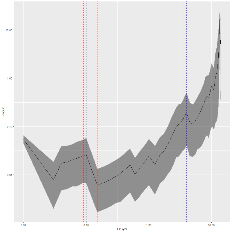
One of my favorite visualization tools for displaying results of star formation history modeling is a ribbon plot of star formation rate versus look back time. This simply plots the marginal posterior mean or median SFR along with 2.5 and 97.5th percentiles (by default) as the lower and upper boundaries of the ribbon. I’ve been using the simplest possible definition of the star formation rate, namely the total mass born in each age bin divided by the interval between the nominal age of each SSP model and the next younger. One striking feature of these plots that’s especially evident in grids of SFH models for an entire galaxy like the one shown in my last post is that there are invariably jumps in the SFR at certain specific ages as marked below. This particular example is from a sample of passively evolving Coma cluster galaxies, but the same features are seen regardless of the likely “true” star formation history.
Star formation rate history estimate – emiles with BaSTI isochrones
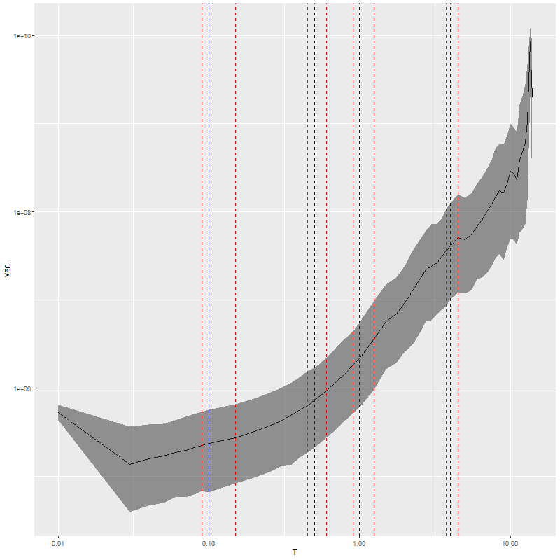
These jumps are artifacts of course: the BaSTI isochrones used for the EMILES SSP models that I currently use are tabulated at age intervals that are constant over certain age ranges, with jumps at 4 ages1100 Myr, 500 Myr, 1 Gyr, and 4 Gyr. The jumps in model SFR occur exactly at the breaks in the age intervals. This turns out to be due to an otherwise welcome feature of the SFH models that they “want” to produce SSP contributions that vary smoothly with age as shown below for the same model run. So for example the stellar mass born in the 90-100 Myr age bin per the model is about 90% of that in the 100-150 Myr bin while the time interval increases by a factor of 5, so the model SFR declines by a factor 4.5 or around 0.6 dex.
Modeled mass born in each age bin – central spectrum of plateifu 9876-12702
Can I do anything about this? Should I? Changing how I calculate the star formation rate might work — this is after all a derivative and I’m currently using the most stupidly simple numerical approximation possible. It also might help to adjust the effective ages of each SSP model. I should also look at the priors on the SSP model coefficients, although as I noted some time ago it’s hard to affect the model star formation histories much with adjustments to priors.
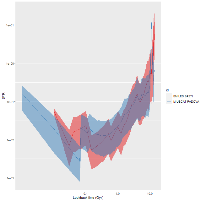
These jumps are something of a peculiarity of the BaSTI isochrones. I had previously used a subset of MILES SSP models from Padova isochrones, which are tabulated at equal logarithmic age intervals. A comparison model run lacks large jumps except for an early time burst. Since the youngest age bin in the Padova isochrones is around 60 Myr I had added two younger SSP models from an update of the BC03 library, and these show abrupt jumps in model SFR. This is also the case with the youngest age bin in my currently used EMILES library.
Comparison of star formation rate history estimates:
Red – EMILES SSP libraries with BaSTI isochrones
Blue – Miuscat SSP library with Padova isochrones
A final comment about these visualizations is that often the mode of the posterior distribution of an SSP model contribution is near 0, and it might make sense to display one sided confidence intervals since what we’re really constraining is an upper limit. I may work on this in the future.
It’s been available for a while actually, but not in a form I’ve been able to figure out how to use. That changed recently with the introduction of the reduce_sum “higher order function” in Stan 2.23.0. What reduce_sum does is allow data to be partitioned into conditionally independent slices that can be dispatched to parallel threads if the Stan program is compiled with threading enabled. My SFH modeling code turns out to be an ideal candidate for parallelization with this technique since flux errors given model coefficients and predictor values are treated as independent1This is an oversimplification since there is certainly some covariance between nearby wavelength bins. This is rarely if ever modeled though and I haven’t figured out how to do it. In any case adding covariance between measurements would complicate matters but not necessarily make it impossible to partition into independent chunks. Here is the line of Stan code that defines the log-likelihood for the current version of my model (see my last post for the complete listing):
This just says the galaxy flux values are drawn from independent gaussians with mean given by the model and known standard deviations. Modifying the code for reduce_sum requires a function to compute a partial sum over any subset of the data for, in this case, the log-likelihood. The partial sum function has to have a specific but fairly flexible function signature. One thing that confused me initially is that the first argument to the partial sum function is a variable to be sliced over that, according to the documentation, must be an array of any type. What was confusing was that passing a variable of vector type as the first argument will fail to compile. In other words a declaration in the data block like
vector[N] y;
with, in the functions block:
real partial_sum(vector y, ...);
fails, while
real y[N];
real partial_sum(real[] y, ...);
works. The problem here is that all of the non-scalar model parameters and data are declared as vector and matrix types because the model involves vector and matrix operations that are more efficiently implemented with high level matrix expressions. Making gflux the sliced variable, which seemed the most obvious candidate, won’t work unless it’s declared as real[] and that won’t work in the sampling statement unless it is cast to a vector since the mean in the expression at the top of the post is a vector. Preliminary investigation with a simpler model indicated that approach works but is so slow that it’s not worth the effort. But, based on a suggestion in the Stan discussion forum a simple trick solved the issue: declare a dummy variable with an array type, pass it as the first argument to the partial sum function, and just don’t use it. So now the partial sum function, which is defined in the functions block is
real sum_ll(int[] ind, int start, int end, matrix sp_st, matrix sp_em,
vector gflux, vector g_std, vector lambda, real a, real tauv, real delta,
vector b_st_s, vector b_em) {
return normal_lpdf(gflux[start:end] | a * (sp_st[start:end, :]*b_st_s) .* calzetti_mod(lambda[start:end], tauv, delta)
+ sp_em[start:end, :]*b_em, g_std[start:end]);
}
I chose to declare the dummy variable ind in a transformed data block. I also declare a tuning variable grainsize there and set it to 1, which tells Stan to set the slice size automatically at run time.
transformed data {
int grainsize = 1;
int ind[nl] = rep_array(1, nl);
}
The rest of the Stan code is the same as presented in the last post.
So why go to this much trouble? As it happens a couple years ago I built a new PC with what was at the time Intel’s second most powerful consumer level CPU, the I9-7960X, which has 16 physical cores and supports 32 threads. I’ve also installed 64GB of DRAM (recently upgraded from 32), which is overkill for most applications but great for running Stan programs which can be rather memory intensive. Besides managing my photo collection I use it for Stan models, but until now I haven’t really been able to make use of its full power. By default Stan runs 4 chains for MCMC sampling, and these can be run in parallel if at least 4 cores are available. It would certainly be possible to run more than 4 chains but this doesn’t buy much: increasing the effective sample size by a factor of 2 or even 4 doesn’t really improve the precision of posterior inferences enough to matter. Once I tried running 16 chains in parallel with a proportionate reduction in post-warmup iterations, but that turned out to be much slower than just using 4 chains. The introduction of reduce_sum raised at least the possibility of making full use of my CPU, and in fact working through the minimal example in Stan’s library of case studies indicated that close to factor of 4 speedups with 4 chains and 4 threads per chain are achievable. I got almost no further improvement setting the threads per chain to 8 and thus using all virtual cores, which apparently is expected at least with Intel CPUs. I haven’t yet tried other combinations, but using all physical cores with the default 4 chains seems likely to be close to optimal. I also haven’t experimented much with the single available tuning parameter, the grainsize. Setting it equal to the sample size divided by 4 and therefore presumably giving each thread an equal size slice did not work better than letting the system set it, in fact it was rather worse IIRC.
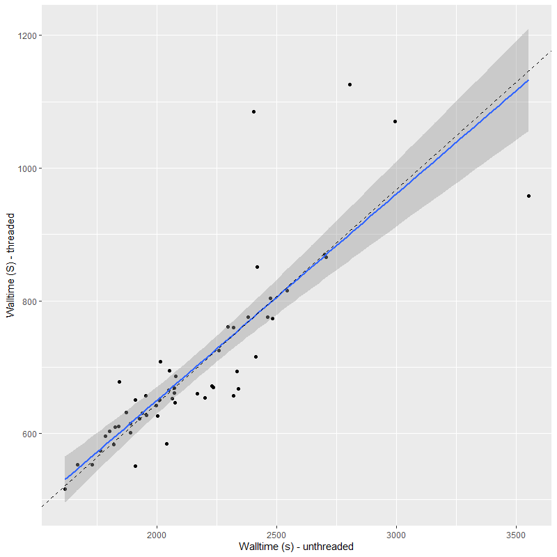
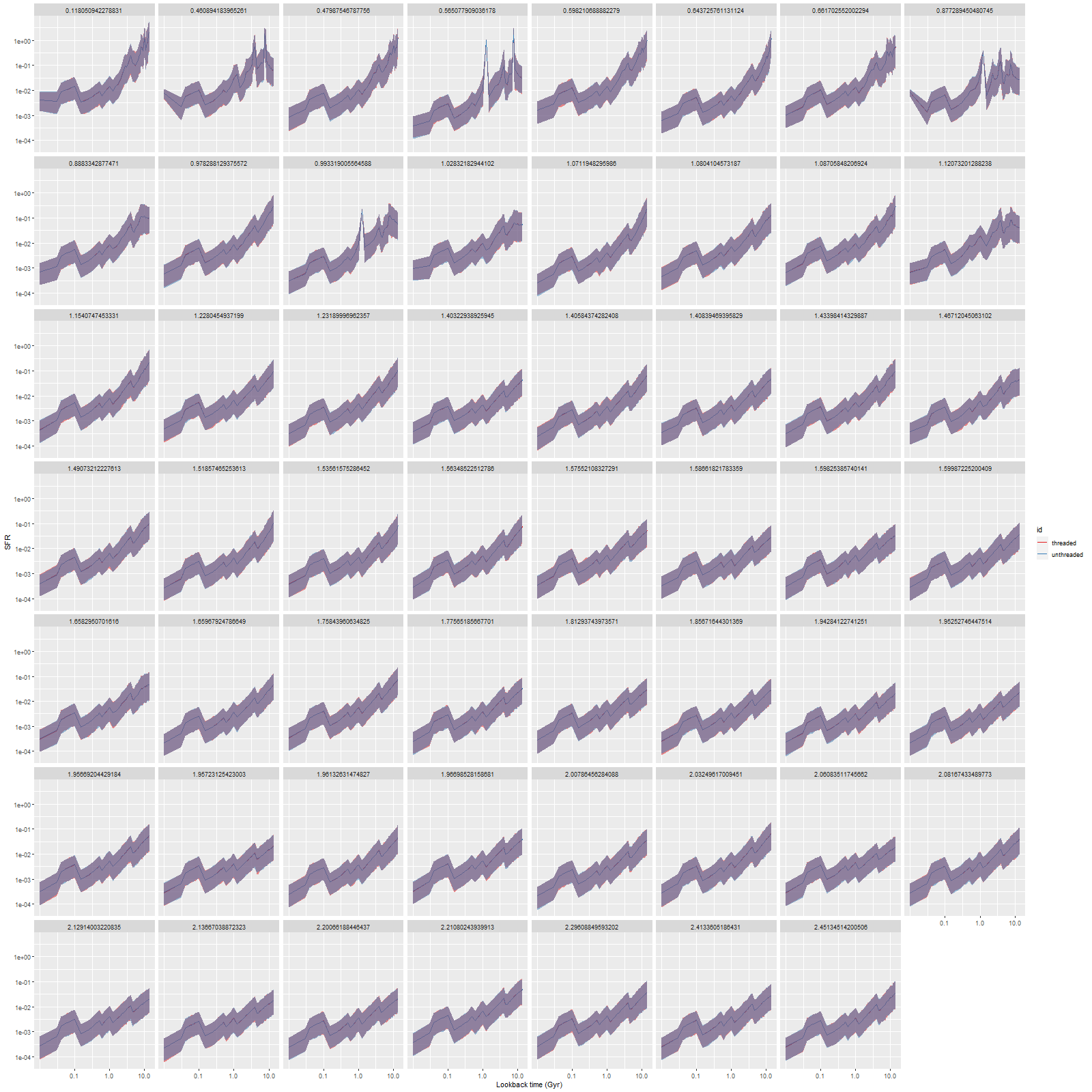
I’ve run both the threaded and unthreaded models on one complete set of data for one MaNGA galaxy. This particular data set used the smallest, 19 fiber IFU, which produces 57 spectra in the stacked RSS data. This was binned to 55 spectra, all with SNR > 5. The galaxy is a passively evolving S0 in or near the Coma cluster, but I’m not going to discuss its star formation history in any detail here. I’m only interested in comparative runtimes and the reproducibility of sampling. And here is the main result of interest, the runtimes (for sampling only) of the threaded and unthreaded code. All runs used 4 chains with 250 warmup iterations and 750 post-warmup. I’ve found 250 warmup iterations to be sufficient almost always and 3000 total samples is more than enough for my purposes. This is actually an increase from what had been my standard practice.
Total execution time for sampling (warmup + post-warmup) in the slowest chain. Graph shows multithreaded vs. threaded time on the same data (N=55 spectra). All threaded runs used 4 chains and 4 threads per chain on a 16 core CPU.
On average the threaded code ran a factor of 3.1 times faster than the unthreaded, and was never worse than about a factor 2 faster2but also never better than a factor 3.7 faster. This is in line with expectations. There’s some overhead involved in threading so speedups are rarely proportional to the number of threads. This is also what I found with the published minimal example and with a just slightly beyond minimal multiple regression model with lots of (fake) data I experimented with. I’ve also found the execution time for these models, particularly in the adaptation phase, to be highly variable with some chains occasionally much faster or slower than others. Stan’s developers are apparently working on communicating between chains during the warmup iterations (they currently do not) and this might reduce between chain disparities in execution time in the future.
I’m mostly interested in model star formation histories, so here’s the comparison of star formation rate densities for both sets of model runs on all 55 bins, ordered by distance from the IFU center (which coincides with the galaxy nucleus):
Star formation rate density. Estimates are for threaded and unthreaded model runs.
Notice that all the ribbons are purple (red + blue), indicating the two sets of runs were nearly enough identical. Exact reproducibility is apparently hard to achieve in multithreaded code, and I didn’t try. I only care about reproducibility within expected Monte Carlo variations, and that was clearly achieved here.
There are only a few down sides to multithreading. The main one is that rstan is currently several dot releases behind Stan itself and seems unlikely to catch up to 2.23.x before 2021. I do extensive pre- and post-processing in R and all of my visualization tools use ggplot2 (an R package) and various extensions. At present the best way to integrate R with a current release of Stan is a (so far) pre-release package called cmdstanr, which bills itself as a “lightweight interface to Stan for R users.” What it actually is is an interface between R and cmdstan, which is in turn the command line driven interface to Stan.
By following directions closely and with a few hints from various sources I was able to install cmdstan from source and with threading support in Windows 10 using Rtools 4.0. The development version of cmdstanr is trivial to install and seems to work exactly as advertised. It is not a drop in replacement for rstan though, and this required me to write some additional functions to fit it into my workflow. Fortunately there’s an rstan function that reads the output files from cmdstan and creates a stanfit object, and this enables me to use virtually all of my existing post-processing code intact.
The other consequence is that cmdstan uses R dump or json format files for input and outputs csv files, the inputs have to be created on the fly, and the outputs have to be read into memory. Cmdstanr with some help from rstan handles this automatically, but there’s some additional overhead compared to rstan which AFAIK keeps all data and sampler output in memory. On my machine the temporary directories reside on a SSD, so all this file I/O goes fairly quickly but still slower than in memory operations. I also worry a bit about the number of read-write cycles but so far the SSD is performing flawlessly.
Multithreading is beneficial to the extent that physical cores are available. This is great for people with access to HPC clusters and it’s helpful to me with an overspec’d and underutilized PC. My current Linux box, which is really better suited to this type of work, only has a several generations old Intel I7 with 4 cores. It’s still a competent and highly reliable machine, but it’s not likely to see any performance improvement from multithreading. Fortunately the current trend is to add more cores to mainstream CPUs: AMD’s Ryzen line currently tops out at 16 cores and their Threadripper series have 24-64 cores. This would be a tempting next build, but alas I’m trying not to spend a lot of money on hobbies these days for more or less obvious reasons.
I’m stranded at sea at the moment so I may as well make a short post. First, here is the complete Stan code of the current model that I’m running. I haven’t gotten around to version controlling this yet or uploading a copy to my github account, so this is the only non-local copy for the moment.
One thing I mentioned in passing way back in this post is that making the stellar contribution parameter vector a simplexseemed to improve sampler performance both in terms of execution time and convergence diagnostics. This was for a toy model where the inputs were nonnegative and summed to one, but it turns out to work better with real data as well. At some point I may want to resurrect old code to document this more carefully, but the main thing I’ve noticed is that post-warmup execution time per sample is often dramatically faster than previously (the execution time for the same number of warmup iterations is about the same or larger though). This appears to be largely due to needing fewer “leapfrog” steps per iteration. It’s fairly common for a model run to have a few “divergent transitions,” which Stan’s developers seem to think is a strong indicator of model failure1I’ve rarely actually seen anything particularly odd about the locations of the divergences and inferences I care about seem unaffected. I’m seeing fewer of these and a larger percentage of model runs with no divergences at all, which indicates the geometry in the unconstrained space may be more favorable.
Here’s the Stan source:
// calzetti attenuation
// precomputed emission lines
functions {
vector calzetti_mod(vector lambda, real tauv, real delta) {
int nl = rows(lambda);
real lt;
vector[nl] fk;
for (i in 1:nl) {
lt = 5500./lambda[i];
fk[i] = -0.10177 + 0.549882*lt + 1.393039*pow(lt, 2) - 1.098615*pow(lt, 3)
+0.260618*pow(lt, 4);
fk[i] *= pow(lt, delta);
}
return exp(-tauv * fk);
}
}
data {
int<lower=1> nt; //number of stellar ages
int<lower=1> nz; //number of metallicity bins
int<lower=1> nl; //number of data points
int<lower=1> n_em; //number of emission lines
vector[nl] lambda;
vector[nl] gflux;
vector[nl] g_std;
real norm_g;
vector[nt*nz] norm_st;
real norm_em;
matrix[nl, nt*nz] sp_st; //the stellar library
vector[nt*nz] dT; // width of age bins
matrix[nl, n_em] sp_em; //emission line profiles
}
parameters {
real a;
simplex[nt*nz] b_st_s;
vector<lower=0>[n_em] b_em;
real<lower=0> tauv;
real delta;
}
model {
b_em ~ normal(0, 100.);
a ~ normal(1, 10.);
tauv ~ normal(0, 1.);
delta ~ normal(0., 0.1);
    gflux ~ normal(a * (sp_st*b_st_s) .* calzetti_mod(lambda, tauv, delta)
                    + sp_em*b_em, g_std);
}
// put in for posterior predictive checking and log_lik
generated quantities {
vector[nt*nz] b_st;
vector[nl] gflux_rep;
vector[nl] mu_st;
vector[nl] mu_g;
vector[nl] log_lik;
real ll;
b_st = a * b_st_s;
mu_st = (sp_st*b_st) .* calzetti_mod(lambda, tauv, delta);
mu_g = mu_st + sp_em*b_em;
for (i in 1:nl) {
gflux_rep[i] = norm_g*normal_rng(mu_g[i] , g_std[i]);
log_lik[i] = normal_lpdf(gflux[i] | mu_g[i], g_std[i]);
mu_g[i] = norm_g * mu_g[i];
}
ll = sum(log_lik);
}
The functions block at the top of the code defines the modified Calzetti attenuation relation that I’ve been discussing in the last several posts. This adds a single parameter delta to the model that acts as a sort of slope difference from the standard curve. As I explained in the last couple posts I give it a tighter prior in the model block than seems physically justified.
There are two sets of parameters for the stellar contributions declared in lines 36-37 of the parameters block. Besides the simplex declaration for the individual SSP contributions there is an overall multiplicative scale parameter a. The way I (re)scale the data, which I’ll get to momentarily, this should be approximately unit valued. This is expressed in the prior in line 44 of the model block. Even though negative values of a would be unphysical I don’t explicitly constrain it since the data should guarantee that almost all posterior probability mass is on the positive side of the real line.
The current version of the code doesn’t have an explicit prior for the simplex valued SSP model contributions which means they have an implicit prior of a maximally dispersed Dirichlet distribution. This isn’t necessarily what I would choose based on domain knowledge and I plan to investigate further, but as I discussed in that post I linked it’s really hard to influence the modeled star formation history much through the choice of prior.
In the MILES SSP models one solar mass is distributed over a given IMF and then allowed to evolve according to one of a choice of stellar isochrones. According to the MILES website the flux units of the model spectra have the peculiar scaling
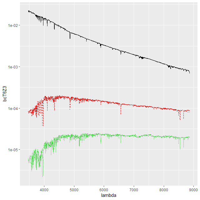
This convention, which is the same as and dates back to at least BC03, is convenient for stellar mass computations since the model coefficient values are proportional to the number of initially solar mass units of each SSP. Calculating quantities like total stellar masses or star formation rates is then a relatively trivial operation. Forward modeling (evolutionary synthesis) is also convenient since there’s a straightforward relationship between star formation histories and predictions for spectra. It may be less convenient for spectrum fitting however, especially using MCMC based methods. The plot below shows a small subset of the SSP library that I’m currently using. Not too surprisingly there’s a multiple order of magnitude range of absolute flux levels with the main source of variation being age. What might be less evident in this plot is that in the units SDSS uses coefficient values might be in the 10’s or hundreds of thousands, with multiple order of magnitude variations among SSP contributors. A simple rescaling of the library spectra to make at least some of the coefficients more nearly unit scaled will address the first problem, but won’t affect the multiple order of magnitude variations among coefficients.
Small sample of EMILES SSP model spectra in original flux units:
T (black): age 1 Myr from 2016 update of BC03 models
M (red) 1 Gyr
B (green) 10 Gyr
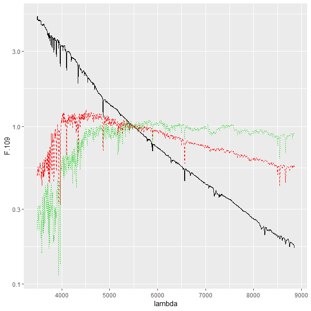
One alternative that’s close to standard statistical practice is to rescale the individual inputs to have approximately the same scale and central value. A popular choice for SED fitting is to normalize to 1 at some fiducial wavelength, often (for UV-optical-NIR data) around V. For my latest model runs I tried renormalizing each SSP spectrum to have a mean value of 1 in a ±150Å window around 5500Å, which happens to be relatively lacking in strong absorption lines at all ages and metallicities.
Same spectra normized to 1 in neighborhood of 5500 Å
This normalization makes the SSP coefficients estimates of light fractions at V, which is intuitively appealing since we are after all fitting light. The effect on sampler performance is hard to predict, but as I said at the top of the post a combination of light weighted fitting with the stellar contribution vector declared as a simplex seems to have favorable performance both in terms of execution time and convergence diagnostics. That’s based on a very small set of model runs and no rigorous performance comparisons at all2among other issues I’ve run versions of these models on at least 4 separate PCs with different generations of Intel processors and both Windows and Linux OSs. This alone produces factor of 2 or more variations in execution time..
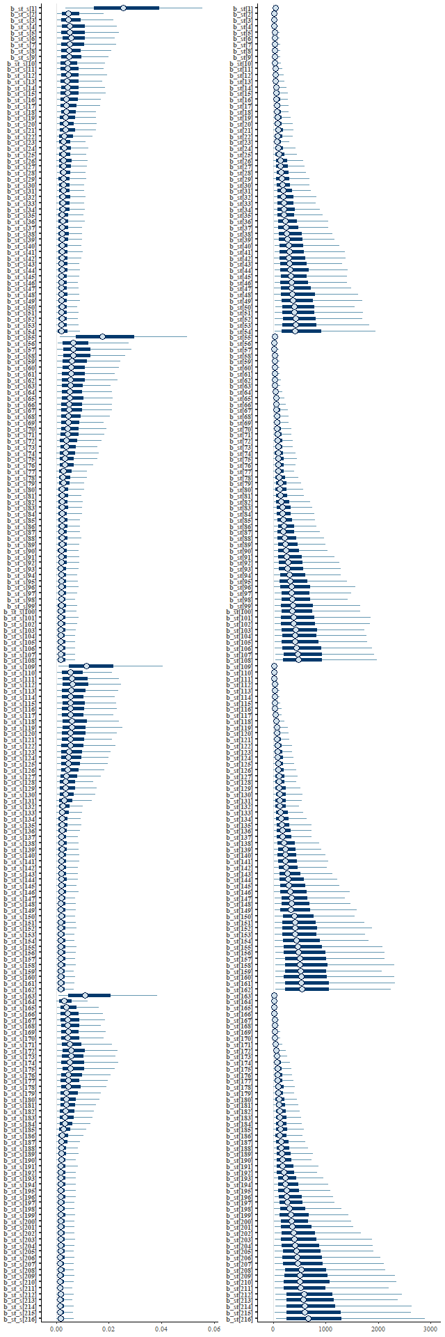
For a quick visual comparison here are coefficient values for a single model run on a spectrum from somewhere in the disk of the spiral galaxy that’s been the subject of the last few posts. These are “interval” plots of the marginal posterior distributions of the SSP model contributions, arranged by metallicity bin (of which there are 4) from lowest to highest and within each bin by age from lowest to highest. The left hand strip of plots are the actual coefficient values representing light fractions at V, while the right hand strip are values proportional to the mass contributions. The latter is what gets transformed into star formation histories and other related quantities. The largest fraction of the light is coming from the youngest populations, which is not untypical for a star forming region. Most of the mass is in older populations, which again is typical.
Another thing that’s very typical is that contributions come from all age and metallicity bins, with similar but not quite identical age trends within each metallicity bin. I find it a real stretch to believe this tells us anything about the real chemical evolution distribution trend with lookback time, but how to interpret this still needs investigation.
Light (L) and mass (R) weighted marginal distributions of coefficient values for a single model run on a disk galaxy spectrum
Here’s an SDSS finder chart image of one of the two grand design spirals that found its way into my “transitional” galaxy sample:
Central galaxy: Mangaid 1-382712 (plateifu 9491-6101), aka CGCG 088-005
and here’s a zoomed in thumbnail with IFU footprint:
plateifu 9491-6101 IFU footprint
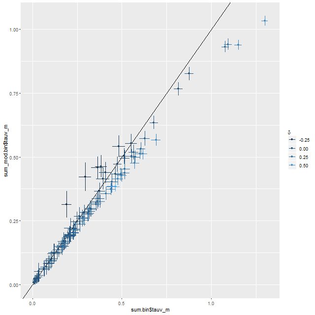
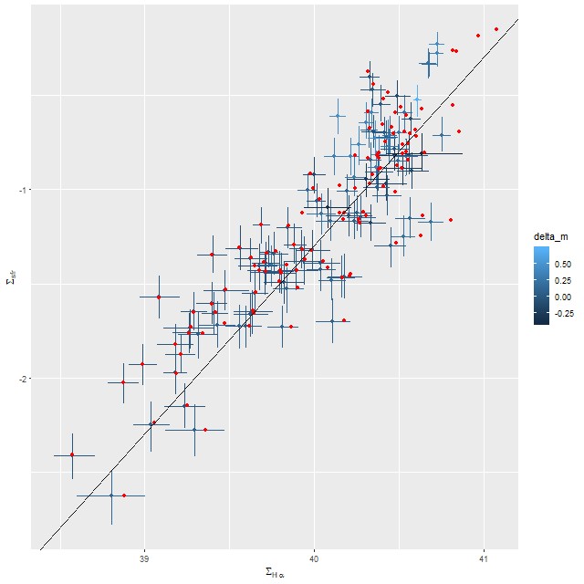
This galaxy is in a compact group and slightly tidally distorted by interaction with its neighbors, but is otherwise a fairly normal star forming system. I picked it because I had a recent set of model runs and because it binned to a manageable but not too small number of spectra (112). The fits to the data in the first set of model runs were good and the (likely) AGN doesn’t have broad lines. Here are a few selected results from the set of model runs using the modified Calzetti attenuation relation on the same binned spectra. First, using a tight prior on the slope parameter δ had the desired effect of returning the prior for δ when τ was near zero, while the marginal posterior for τ was essentially unchanged:
Estimated optical depth for modified Calzetti attenuation vs. unmodified. MaNGA plateifu 9491-6101
At larger optical depths the data do constrain both the shape of the attenuation curve and optical depth. At low optical depth the posterior uncertainty in δ is about the same as the prior, while it decreases more or less monotonically for higher values of τ. A range of (posterior mean) values of δ from slightly shallower than a Calzetti relation to somewhat steeper. The general trend is toward a steeper relation with lower optical depth in the dustier regions (per the models) of the galaxy.
Posterior marginal standard deviation of parameter δ vs. posterior mean optical depth. MaNGA plateifu 9491-6101
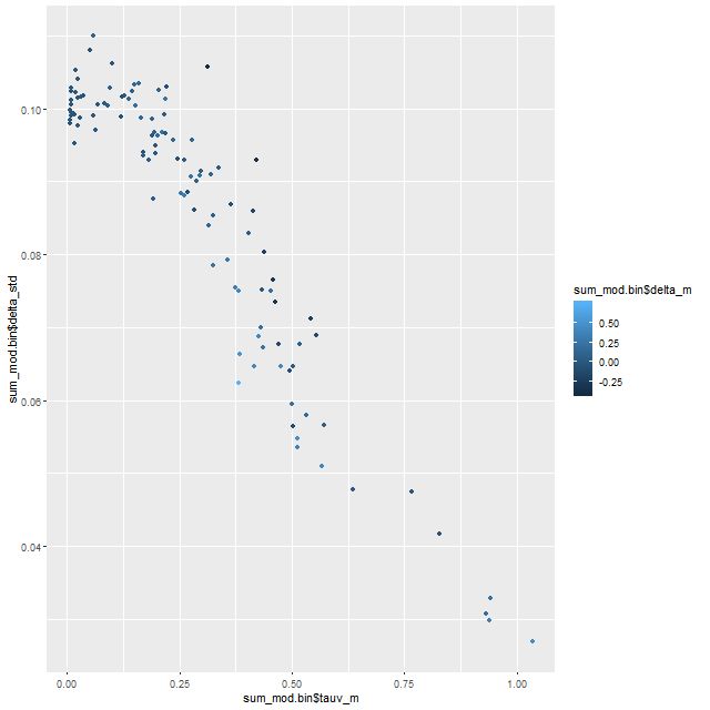
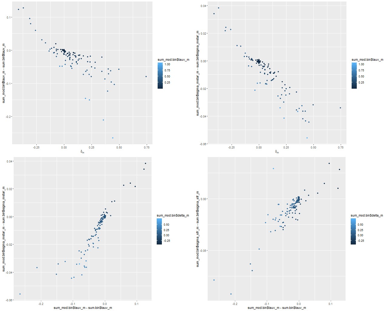
There’s an interesting pattern of correlations1astronmers like to call these “degeneracies,” and it’s fairly well known that they exist among attenuation, stellar age, stellar mass, and other properties here, some of which are summarized in the sequence of plots below. The main result is that a steeper (shallower) attenuation curve requires a smaller (larger) optical depth to create a fixed amount of reddening, so there’s a negative correlation between the slope parameter δ and the change in optical depth between the modified and unmodified curves. A lower optical depth means that a smaller amount of unattenuated light, and therefore lower stellar mass, is needed to produce a given observed flux. so there’s a negative correlation between the slope parameter and stellar mass density or a positive correlation between optical depth and stellar mass. The star formation rate density is correlated in the same sense but slightly weaker. In this data set both changed by less than about ± 0.05 dex.
(TL) change in optical depth (modified – unmodified calzetti) vs. slope parameter δ (TR) change in stellar mass density vs. δ (BL) change in stellar mass density vs. change in optical depth (BR) change in SFR density vs change in optical depth Note: all quantities are marginal posterior mean estimagtes.
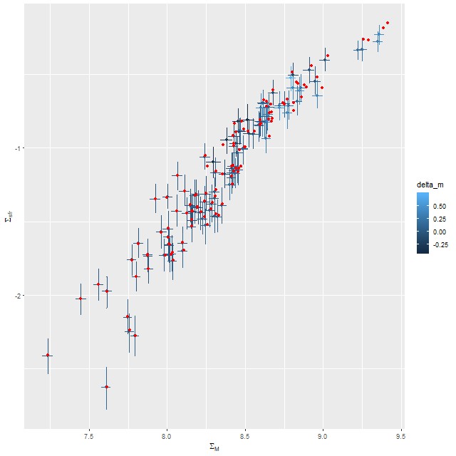
Here are a few relationships that I’ve shown previously. First between stellar mass and star formation rate density. The points with error bars (which are 95% marginal credible limits) are from the modified Calzetti run, while the red points are from the original. Regions with small stellar mass density and low star formation rate have small attenuation as well in this system, so the estimates hardly differ at all. Only at the high end are differences about as large as the nominal uncertainties.
SFR density vs. stellar mass density. Red points are point estimates for unmodified Calzetti attenuation. MaNGA plateifu 9491-6101
Finally, here is the relation between Hα luminosity density and star formation rate with the former corrected for attenuation using the Balmer decrement. The straight line is, once again, the calibration of Moustakas et al. Allowing the shape of the attenuation curve to vary has a larger effect on the luminosity correction than it does on the SFR estimates, but both sets of estimates straddle the line with roughly equal scatter.
SFR density vs. Hα luminosity density. Red points are point estimates for unmodified Calzetti attenuation.
MaNGA plateifu 9491-6101
To conclude for now, adding the more flexible attenuation prescription proposed by Salim et al. has some quantitative effects on model posteriors, but so far at least qualitative inferences aren’t significantly affected. I haven’t yet looked in detail at star formation histories or at effects on metallicity or metallicity evolution. I’ve been skeptical that SFH modeling constrains stellar metallicity or (especially) metallicity evolution well, but perhaps it’s time to take another look.
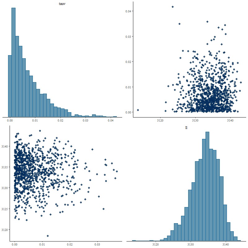
Here’s a problem that isn’t a huge surprise but that I hadn’t quite anticipated. I initially chose, without a lot of thought, a prior \(\delta \sim \mathcal{N}(0, 0.5)\) for the slope parameter delta in the modified Calzetti relation from the last post. This seemed reasonable given Salim et al.’s result showing that most galaxies have slopes \(-0.1 \lesssim \delta \lesssim +1\) (my wavelength parameterization reverses the sign of \(\delta\) ). At the end of the last post I made the obvious comment that if the modeled optical depth is near 0 the data can’t constrain the shape of the attenuation curve and in that case the best that can be hoped for is the model to return the prior for delta. Unfortunately the actual model behavior was more complicated than that for a spectrum that had a posterior mean tauv near 0:
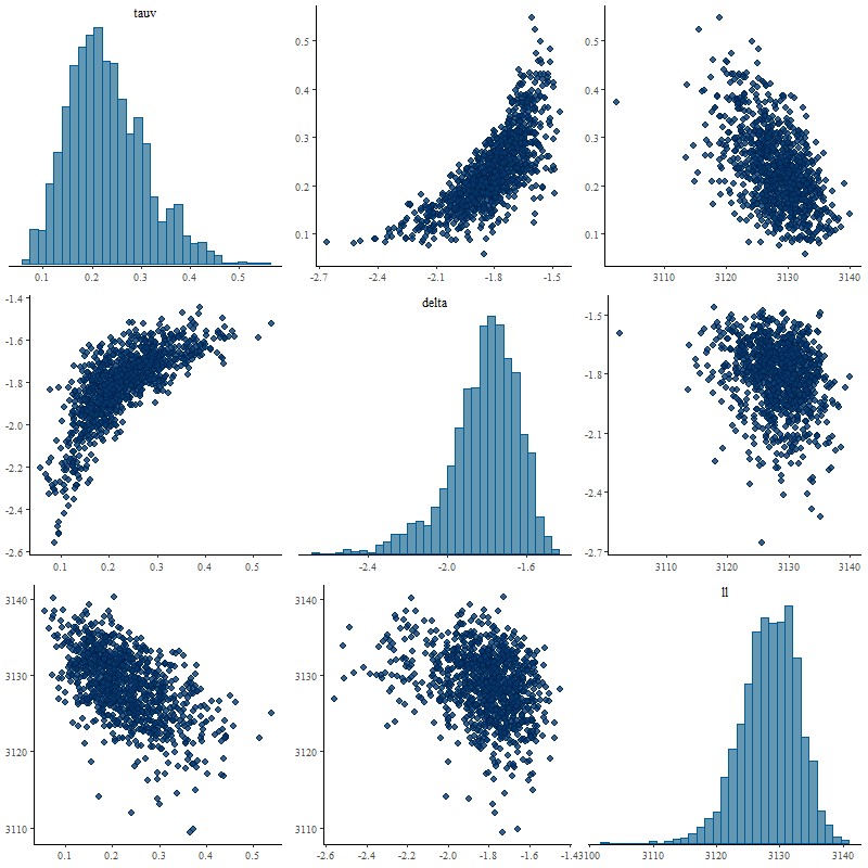
Pairs plot of parameters tauv and delta, plus summed log likelihood with “loose” prior on delta.
Although there weren’t any indications of convergence issues in this run experts in the Stan community often warn that “banana” shaped posteriors like the joint distribution of tauv and delta above are difficult for the HMC algorithm in Stan to explore. I also suspect the distribution is multi-modal and at least one mode was missed, since the fit to the flux data as indicated by the summed log-likelihood is slightly worse than the unmodified Calzetti model.
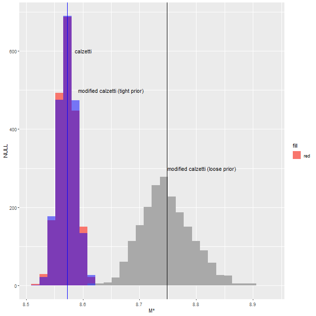
A value of \(\delta\) this small actually reverses the slope of the attenuation curve, making it larger in the red than in the blue. It also resulted in a stellar mass estimate about 0.17 dex larger than the original model, which is well outside the statistical uncertainty:
Stellar mass estimates for loose and tight priors on delta + unmodified Calzetti attenuation curve
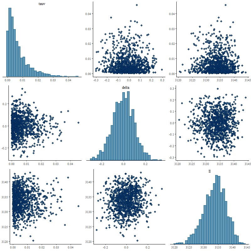
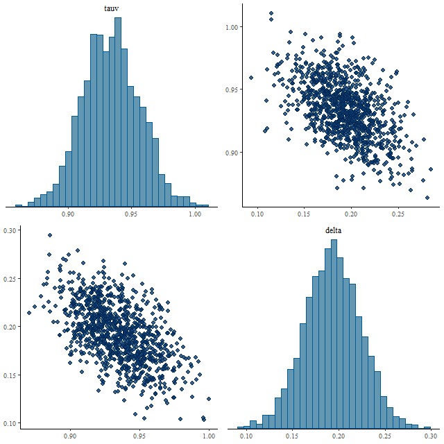
I next tried a tighter prior on delta of 0.1 for the scale parameter, with the following result:
Pairs plot of parameters tauv and delta, plus summed log likelihood with “tight” prior on delta.
Now this is what I hoped to see. The marginal posterior of delta almost exactly returns its prior, properly reflecting the inability of the data to say anything about it. The posterior of tauv looks almost identical to the original model with a very slightly longer tail:
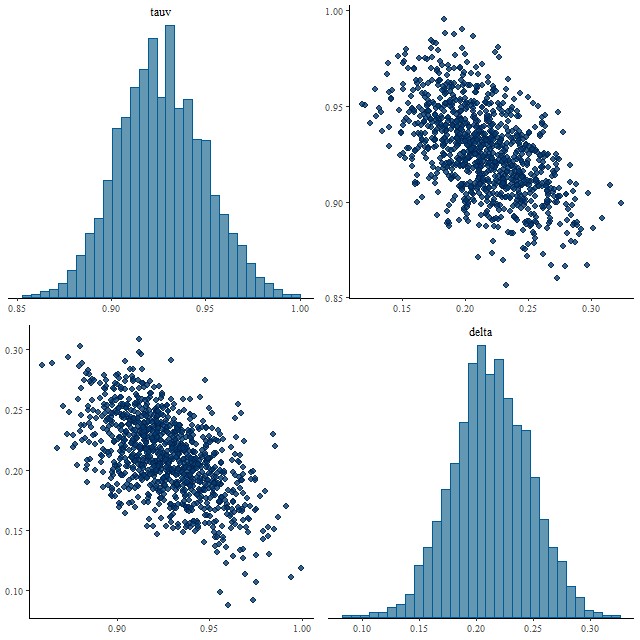
Pairs plot of parameters tauv and summed log likelihood, unmodified Calzetti attenuation curve
So this solves one problem but now I must worry that the prior is too tight in general since Salim’s results predict a considerably larger spread of slopes. As a first tentative test I ran another spectrum from the same spiral galaxy (this is mangaid 1-382712) that had moderately large attenuation in the original model (1.08 ± 0.04) with both “tight” and “loose” priors on delta with the following results:
Joint posterior of parameters tau and delta with “tight” priorJoint posterior of parameters tau and delta with “loose” prior
The distributions of tauv look nearly the same, while delta shrinks very slightly towards 0 with a tight prior, but with almost the same variance. Some shrinkage towards Calzetti’s original curve might be OK. Anyway, on to a larger sample.
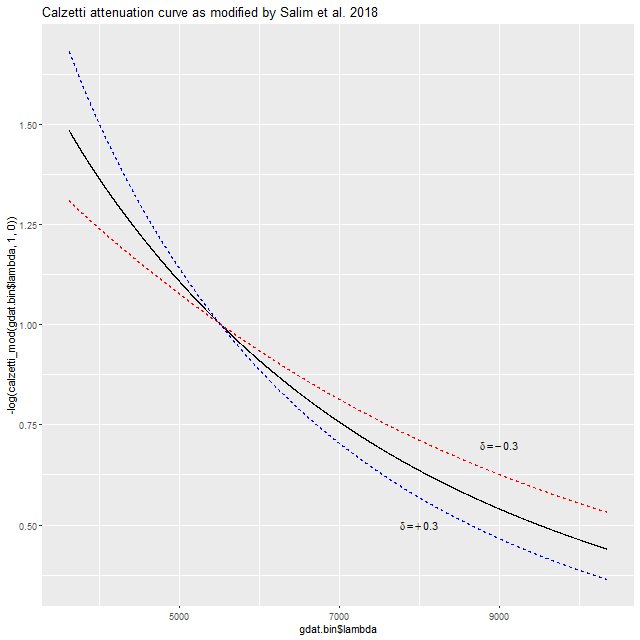
I finally got around to reading a paper by Salim, Boquien, and Lee (2018), who proposed a simple modification to Calzetti‘s well known starburst attenuation relation that they claim accounts for most of the diversity of curves in both star forming and quiescent galaxies. For my purposes their equation 3, which summarizes the relation, can be simplified in two ways. First, for mostly historical reasons optical astronomers typically quantify the effect of dust with a color excess, usually E(B-V). If the absolute attenuation is needed, which is certainly the case in SFH modeling, the ratio of absolute to “selective” attenuation, usually written as \(\mathrm{R_V = A_V/E(B-V)}\) is needed. Parameterizing attenuation by color excess adds an unnecessary complication for my purposes. Salim et al. use a family of curves that differ only in a “slope” parameter \(\delta\) in their notation. Changing \(\delta\) changes \(\mathrm{R_V}\) according to their equation 4. But I have always parametrized dust attenuation by optical depth at V, \(\tau_V\) so that the relation between intrinsic and observed flux is
Note that parameterizing by optical depth rather than total attenuation \(\mathrm{A_V}\) is just a matter of taste since they only differ by a factor 1.08. The wavelength dependent part of the relationship is the same.
The second simplification results from the fact that the UV or 2175Å “bump” in the attenuation curve will never be redshifted into the spectral range of MaNGA data and in any case the subset of the EMILES library I currently use doesn’t extend that far into the UV. That removes the bump amplitude parameter and the second term in Salim et al.’s equation 3, reducing it to the form
The published expression for \(k(\lambda)\) in Calzetti et al. (2000) is given in two segments with a small discontinuity due to rounding at the transition wavelength of 6300Å. This produces a small unphysical discontinuity when applied to spectra, so I just made a polynomial fit to the Calzetti curve over a longer wavelength range than gets used for modeling MaNGA or SDSS data. Also, I make the wavelength parameter \(y = 5500/\lambda\) instead of using the wavelength in microns as in Calzetti. With these adjustments Calzetti’s relation is, to more digits than necessary:
Note that δ has the opposite sign as in Salim et al. Here is what the curve looks like over the observer frame wavelength range of MaNGA. A positive value of δ produces a steeper attenuation curve than Calzetti’s, while a negative value is shallower (grayer in common astronomers’ jargon). Salim et al. found typical values to range between about -0.1 and +1.
Calzetti attenuation relation with modification proposed by Salim, Boquien, and Lee (2018). Dashed lines show shift in curve for their parameter δ = ± 0.3.
For a first pass attempt at modeling some real data I chose a spectrum from near the northern nucleus of Mrk 848 but outside the region of the highest velocity outflows. This spectrum had large optical depth \(\tau_V \approx 1.52\) and the unusual nature of the galaxy gave reason to think its extinction curve might differ significantly from Calzetti’s.
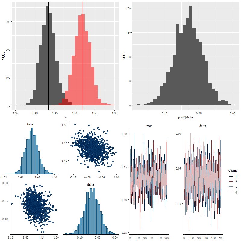
Encouragingly, the Stan model converged without difficulty and with an acceptable run time. Below are some posterior plots of the two attenuation parameters and a comparison to the optical depth parameter in the unmodified Calzetti dust model. I used a fairly informative prior of Normal(0, 0.5) for the parameter delta. The data actually constrain the value of delta, since its posterior marginal density is centered around -0.06 with a standard deviation of just 0.02. In the pairs plot below we can see there’s some correlation between the posteriors of tauv and delta, but not so much as to be concerning (yet).
(TL) marginal posteriors of optical depth parameter for Calzetti (red) and modified (dark gray) relation.
(TR) parameter δ in modified Calzetti relation
(BL) pairs plot of `tauv` and `delta`
(BR) trace plots of `tauv` and `delta`
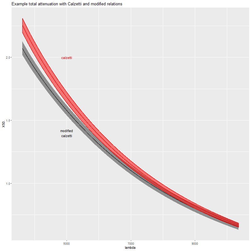
Overall the modified Calzetti model favors a slightly grayer attenuation curve with lower absolute attenuation:
Total attenuation for original and modified Calzetti relations. Spectrum was randomly selected near the northern nucleus or Mrk 848.
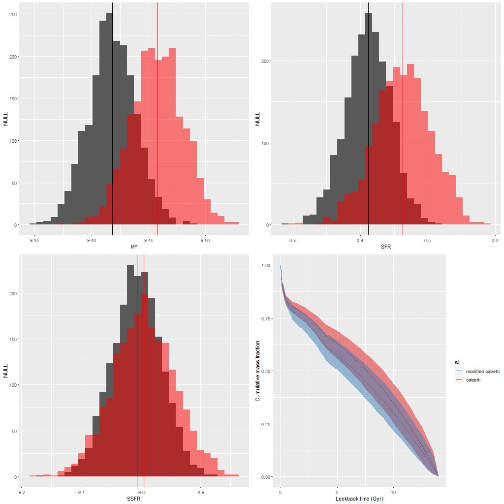
Here’s a quick look at the effect of the model modification on some key quantities. In the plot below the red symbols are for the unmodified Calzetti attenuation model, and gray or blue the modified one. These show histograms of the marginal posterior density of total stellar mass, 100Myr averaged star formation rate, and specific star formation rate. Because the modified model has lower total attenuation it needs fewer stars, so the lower stellar mass (by ≈ 0.05 dex) is a fairly predictable consequence. The star formation rate is also lower by a similar amount, making the estimates of specific star formation rate nearly identical.
The lower right pane compares model mass growth histories. I don’t have any immediate intuition about how the difference in attenuation models affects the SFH models, but notice that both show recent acceleration in star formation, which was a main theme of my Markarian 848 posts.
Stellar mass, SFR,, SSFR, and mass growth histories for original and modified Calzetti attenuation relation.
So, this first run looks ok. Of course the problem with real data is there’s no way to tell if a model modification actually brings it closer to reality — in this case it did improve the fit to the data a little bit (by about 0.2% in log likelihood) but some improvement is expected just from adding a parameter.
My concern right now is that if the dust attenuation is near 0 the data can’t constrain the value of δ. The best that can happen in this situation is for the model to return the prior. Preliminary investigation of a low attenuation spectrum (per the original model) suggests that in fact a tighter prior on delta is needed than what I originally chose.