
I finally got around to reading a paper by Salim, Boquien, and Lee (2018), who proposed a simple modification to Calzetti‘s well known starburst attenuation relation that they claim accounts for most of the diversity of curves in both star forming and quiescent galaxies. For my purposes their equation 3, which summarizes the relation, can be simplified in two ways. First, for mostly historical reasons optical astronomers typically quantify the effect of dust with a color excess, usually E(B-V). If the absolute attenuation is needed, which is certainly the case in SFH modeling, the ratio of absolute to “selective” attenuation, usually written as \(\mathrm{R_V = A_V/E(B-V)}\) is needed. Parameterizing attenuation by color excess adds an unnecessary complication for my purposes. Salim et al. use a family of curves that differ only in a “slope” parameter \(\delta\) in their notation. Changing \(\delta\) changes \(\mathrm{R_V}\) according to their equation 4. But I have always parametrized dust attenuation by optical depth at V, \(\tau_V\) so that the relation between intrinsic and observed flux is
\(F_o(\lambda) = F_i(\lambda) \mathrm{e}^{-\tau_V k(\lambda)}\)
Note that parameterizing by optical depth rather than total attenuation \(\mathrm{A_V}\) is just a matter of taste since they only differ by a factor 1.08. The wavelength dependent part of the relationship is the same.
The second simplification results from the fact that the UV or 2175Å “bump” in the attenuation curve will never be redshifted into the spectral range of MaNGA data and in any case the subset of the EMILES library I currently use doesn’t extend that far into the UV. That removes the bump amplitude parameter and the second term in Salim et al.’s equation 3, reducing it to the form
\(k_{mod}(\lambda) = k_{Cal}(\lambda)(\frac{\lambda}{5500})^\delta\)
The published expression for \(k(\lambda)\) in Calzetti et al. (2000) is given in two segments with a small discontinuity due to rounding at the transition wavelength of 6300Å. This produces a small unphysical discontinuity when applied to spectra, so I just made a polynomial fit to the Calzetti curve over a longer wavelength range than gets used for modeling MaNGA or SDSS data. Also, I make the wavelength parameter \(y = 5500/\lambda\) instead of using the wavelength in microns as in Calzetti. With these adjustments Calzetti’s relation is, to more digits than necessary:
\(k_{Cal}(y) = -0.10177 + 0.549882y + 1.393039 y^2 – 1.098615 y^3 + 0.260628 y^4\)
and Salim’s modified curve is
\(k_{mod}(\lambda) = k_{Cal}(\lambda)y^\delta\)
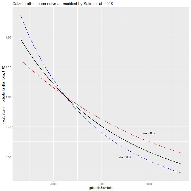
Note that δ has the opposite sign as in Salim et al. Here is what the curve looks like over the observer frame wavelength range of MaNGA. A positive value of δ produces a steeper attenuation curve than Calzetti’s, while a negative value is shallower (grayer in common astronomers’ jargon). Salim et al. found typical values to range between about -0.1 and +1.
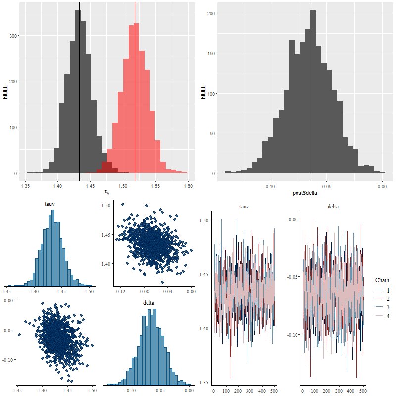
For a first pass attempt at modeling some real data I chose a spectrum from near the northern nucleus of Mrk 848 but outside the region of the highest velocity outflows. This spectrum had large optical depth \(\tau_V \approx 1.52\) and the unusual nature of the galaxy gave reason to think its extinction curve might differ significantly from Calzetti’s.
Encouragingly, the Stan model converged without difficulty and with an acceptable run time. Below are some posterior plots of the two attenuation parameters and a comparison to the optical depth parameter in the unmodified Calzetti dust model. I used a fairly informative prior of Normal(0, 0.5) for the parameter delta. The data actually constrain the value of delta, since its posterior marginal density is centered around -0.06 with a standard deviation of just 0.02. In the pairs plot below we can see there’s some correlation between the posteriors of tauv and delta, but not so much as to be concerning (yet).
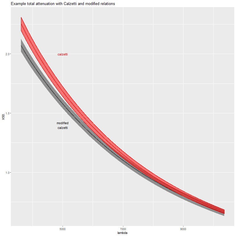
Overall the modified Calzetti model favors a slightly grayer attenuation curve with lower absolute attenuation:
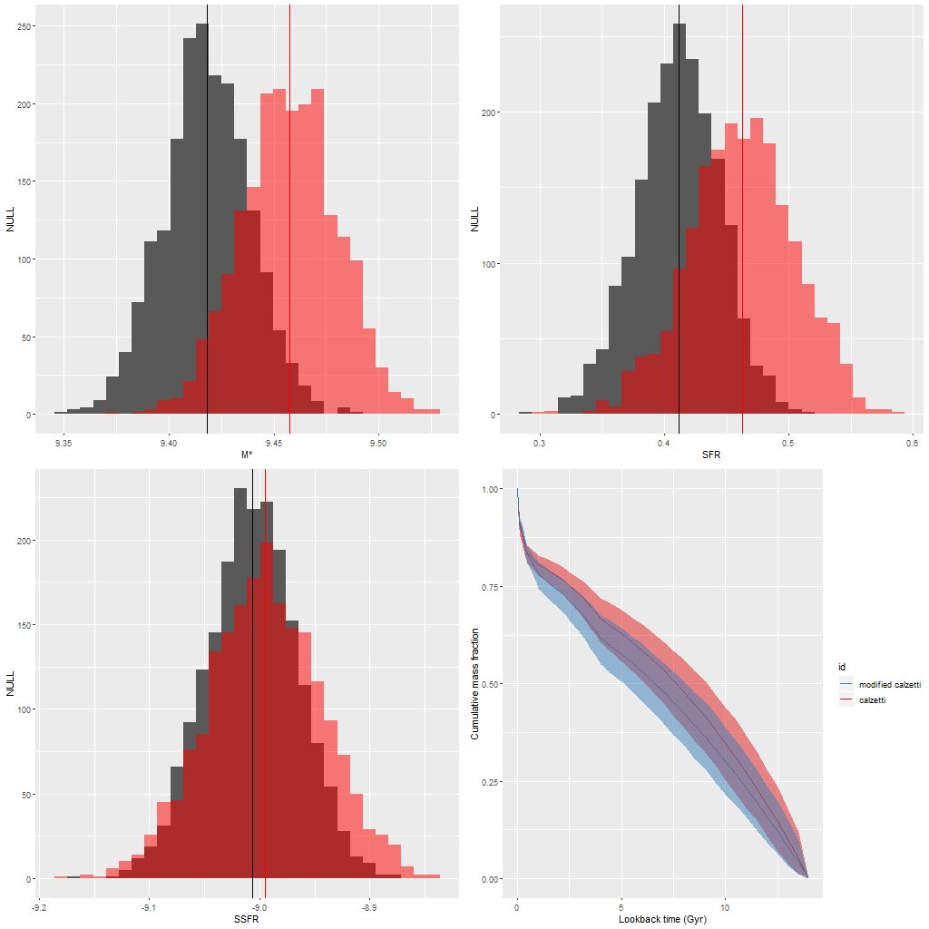
Here’s a quick look at the effect of the model modification on some key quantities. In the plot below the red symbols are for the unmodified Calzetti attenuation model, and gray or blue the modified one. These show histograms of the marginal posterior density of total stellar mass, 100Myr averaged star formation rate, and specific star formation rate. Because the modified model has lower total attenuation it needs fewer stars, so the lower stellar mass (by ≈ 0.05 dex) is a fairly predictable consequence. The star formation rate is also lower by a similar amount, making the estimates of specific star formation rate nearly identical.
The lower right pane compares model mass growth histories. I don’t have any immediate intuition about how the difference in attenuation models affects the SFH models, but notice that both show recent acceleration in star formation, which was a main theme of my Markarian 848 posts.
So, this first run looks ok. Of course the problem with real data is there’s no way to tell if a model modification actually brings it closer to reality — in this case it did improve the fit to the data a little bit (by about 0.2% in log likelihood) but some improvement is expected just from adding a parameter.
My concern right now is that if the dust attenuation is near 0 the data can’t constrain the value of δ. The best that can happen in this situation is for the model to return the prior. Preliminary investigation of a low attenuation spectrum (per the original model) suggests that in fact a tighter prior on delta is needed than what I originally chose.