A simple Bayesian model for linear regression with measurement errors

Here’s a pretty common situation with astronomical data: two or more quantities are measured with nominally known uncertainties that in general will differ between observations. We’d like to explore the relationship among them, if any. After graphing the data and establishing that there is a relationship a first cut quantitative analysis would usually be a linear regression model fit to the data. But the ordinary least squares fit is biased and might be severely misleading if the measurement errors are large enough. I’m going to present a simple measurement error model formulation that’s amenable to Bayesian analysis and that I’ve implemented in Stan. This model is not my invention by the way — in the astronomical literature it dates at least to Kelly (2007), who also explored a number of generalizations. I’m only going to discuss the simplest case of a single predictor or covariate, and I’m also going to assume all conditional distributions are gaussian.

The basic idea of the model is that the real, unknown quantities (statisticians call these latent variables, and so will I) are related through a linear regression. The conditional distribution of the latent dependent variable is

\(y^{lat}_i | x^{lat}_i, \beta_0, \beta_1, \sigma \sim \mathcal{N}(\beta_0 + \beta_1 x^{lat}_i, \sigma)~~~ i = 1, \cdots, N\)

The observed values then are generated from the latent ones with distributions

\(y^{obs}_i| y^{lat}_i \sim \mathcal{N}(y^{lat}_i, \sigma_{y, i})\)

\(x^{obs}_i| x^{lat}_i \sim \mathcal{N}(x^{lat}_i, \sigma_{x, i})~~~ i = 1, \cdots, N\)

where \(\sigma_{x, i}, \sigma_{y, i}\) are the known standard deviations. The full joint distribution is completed by specifying priors for the parameters \(\beta_0, \beta_1, \sigma\). This model is very easy to implement in the Stan language and the complete code is listed below. I’ve also uploaded the code, a script to reproduce the simulated data example discussed below, and the SFR-stellar mass data from the last page in a dropbox folder.

/**
 * Simple regression with measurement error in x and y
*/

data {
  int<lower=0> N;
  vector[N] x;
  vector<lower=0>[N] sd_x;
  vector[N] y;
  vector<lower=0>[N] sd_y;
} 

// standardize data
transformed data {
  real mean_x = mean(x);
  real sd_xt = sd(x);
  real mean_y = mean(y);
  real sd_yt = sd(y);
  
  vector[N] xhat = (x - mean_x)/sd_xt;
  vector<lower=0>[N] sd_xhat = sd_x/sd_xt;
  
  vector[N] yhat = (y - mean_y)/sd_yt;
  vector<lower=0>[N] sd_yhat = sd_y/sd_yt;
  
}


parameters {
  vector[N] x_lat;
  vector[N] y_lat;
  real beta0;
  real beta1;
  real<lower=0> sigma;
}
transformed parameters {
  vector[N] mu_yhat = beta0 + beta1 * x_lat;
}
model {
  x_lat ~ normal(0., 1000.);
  beta0 ~ normal(0., 5.);
  beta1 ~ normal(0., 5.);
  sigma ~ normal(0., 10.);
  
  xhat ~ normal(x_lat, sd_xhat);
  y_lat ~ normal(mu_yhat, sigma);
  yhat ~ normal(y_lat, sd_yhat);
  
} 

generated quantities {
  vector[N] xhat_new;
  vector[N] yhat_new;
  vector[N] y_lat_new;
  vector[N] x_new;
  vector[N] y_new;
  vector[N] mu_x;
  vector[N] mu_y;
  real b0;
  real b1;
  real sigma_unorm;
  
  b0 = mean_y + sd_yt*beta0 - beta1*sd_yt*mean_x/sd_xt;
  b1 = beta1*sd_yt/sd_xt;
  sigma_unorm = sd_yt * sigma;
  
  mu_x = x_lat*sd_xt + mean_x;
  mu_y = mu_yhat*sd_yt + mean_y;
  
  for (n in 1:N) {
    xhat_new[n] = normal_rng(x_lat[n], sd_xhat[n]);
    y_lat_new[n] = normal_rng(beta0 + beta1 * x_lat[n], sigma);
    yhat_new[n] = normal_rng(y_lat_new[n], sd_yhat[n]);
    x_new[n] = sd_xt * xhat_new[n] + mean_x;
    y_new[n] = sd_yt * yhat_new[n] + mean_y;
  }
}

Most of this code should be self explanatory, but there are a few things to note. In the transformed data section I standardize both variables, that is I subtract the means and divide by the standard deviations. The individual observation standard deviations are also scaled. The transformed parameters block is strictly optional in this model. All it does is spell out the linear part of the linear regression model.

In the model block I give a very vague prior for the latent x variables. This has almost no effect on the model output since the posterior distributions of the latent values are strongly constrained by the observed data. The parameters of the regression model are given less vague priors. Since we standardized the data we know beta0 should be centered near 0 and beta1 near 1 and all three should be approximately unit scaled. The rest of the model block just encodes the conditional distributions I wrote out above.

Finally the generated quantities block does two things: generate some some new simulated data values under the model using the sampled parameters, and rescale the parameter values to the original data scale. The first task enables what’s called “posterior predictive checking.” Informally the idea is that if the model is successful simulated data generated under it should look like the data that was input.

It’s always a good idea to try out a model with some simulated data that conforms to it, so here’s a script to generate some data, then print and graph some basic results. This is also in the dropbox folder.

testme <- function(N=200, mu_x=0, b0=10, b1=2, sigma=0.5, seed1=1234, seed2=23455, ...) {
  require(rstan)
  require(ggplot2)
  set.seed(seed1)
  x_lat <- rnorm(N, mean=mu_x, sd=1.)
  sd_x <- runif(N, min=0.1, max=0.2)
  sd_y <- runif(N, min=0.1, max=0.2)
  x_obs <- x_lat+rnorm(N, sd=sd_x)
  y_lat <- b0 + b1*x_lat + rnorm(N, sd=sigma)
  y_obs <- y_lat + rnorm(N, sd=sd_y)
  stan_dat <- list(N=N, x=x_obs, sd_x=sd_x, y=y_obs, sd_y=sd_y)
  df1 <- data.frame(x_lat=x_lat, x=x_obs, sd_x=sd_x, y_lat=y_lat, y=y_obs, sd_y=sd_y)
  sfit <- stan(file="ls_me.stan", data=stan_dat, seed=seed2, chains=4, cores=4, ...)
  print(sfit, pars=c("b0", "b1", "sigma_unorm"), digits=3)
  g1 <- ggplot(df1)+geom_point(aes(x=x, y=y))+geom_errorbar(aes(x=x,ymin=y-sd_y,ymax=y+sd_y)) +
                      geom_errorbarh(aes(y=y, xmin=x-sd_x, xmax=x+sd_x))
  post <- extract(sfit)
  df2 <- data.frame(x_new=as.numeric(post$x_new), y_new=as.numeric(post$y_new))
  g1 <- g1 + stat_ellipse(aes(x=x_new, y=y_new), data=df2, geom="path", type="norm", linetype=2, color="blue") +
            geom_abline(slope=post$b1, intercept=post$b0, alpha=1/100)
  plot(g1)
  list(sfit=sfit, stan_dat=stan_dat, df=df1, graph=g1)
}
  

This should print the following output:

Inference for Stan model: ls_me.
4 chains, each with iter=2000; warmup=1000; thin=1; 
post-warmup draws per chain=1000, total post-warmup draws=4000.

             mean se_mean    sd  2.5%   25%   50%    75%  97.5% n_eff  Rhat
b0          9.995   0.001 0.042 9.912 9.966 9.994 10.023 10.078  5041 0.999
b1          1.993   0.001 0.040 1.916 1.965 1.993  2.020  2.073  4478 1.000
sigma_unorm 0.472   0.001 0.037 0.402 0.447 0.471  0.496  0.549  2459 1.003

Samples were drawn using NUTS(diag_e) at Thu Jan  9 10:09:34 2020.
For each parameter, n_eff is a crude measure of effective sample size,
and Rhat is the potential scale reduction factor on split chains (at 
convergence, Rhat=1).
> 

and graph:

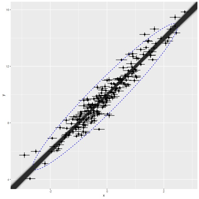
This all looks pretty good. The true parameters are well within the 95% confidence bounds of the estimates. In the graph the simulated new data is summarized with a 95% confidence ellipse, which encloses just about 95% of the input data, so the posterior predictive check indicates a good model. Stan is quite aggressive at flagging potential convergence failures, and no warnings were generated.

Turning to some real data I also included in the dropbox folder the star formation rate density versus stellar mass density data that I discussed in the last post. This is in something called R “dump” format, which is just an ascii file with R assignment statements for the input data. This isn’t actually a convenient form for input to rstan’s sampler or ggplot2’s plotting commands, so once loaded the data are copied into a list and a data frame. The interactive session for analyzing the data was:

 source("sf_mstar_sfr.txt")
> sf_dat <- list(N=N, x=x, sd_x=sd_x, y=y, sd_y=sd_y)
> df <- data.frame(x=x,sd_x=sd_x,y=y,sd_y=sd_y)
> stan_sf <- stan(file="ls_me.stan",data=sf_dat, chains=4,seed=12345L)

 post <- extract(stan_sf)
> odr <- pracma::odregress(df$x,df$y)
> ggplot(df, aes(x=x,y=y))+geom_point()+geom_errorbar(aes(x=x,ymin=y-sd_y,ymax=y+sd_y))+geom_errorbarh(aes(y=y,xmin=x-sd_x,xmax=x+sd_x))+geom_abline(slope=post$b1,intercept=post$b0,alpha=1/100)+stat_ellipse(aes(x=x_new,y=y_new),data=data.frame(x_new=as.numeric(post$x_new),y_new=as.numeric(post$y_new)),geom="path",type="norm",linetype=2, color="blue")+geom_abline(slope=odr$coef[1],intercept=odr$coef[2],color='red',linetype=2)
> print(stan_sf, pars=c("b0","b1","sigma_unorm"))

 

Inference for Stan model: ls_me.
4 chains, each with iter=2000; warmup=1000; thin=1; 
post-warmup draws per chain=1000, total post-warmup draws=4000.

              mean se_mean   sd   2.5%    25%    50%    75%  97.5% n_eff Rhat
b0          -11.20       0 0.26 -11.73 -11.37 -11.19 -11.02 -10.67  7429    1
b1            1.18       0 0.03   1.12   1.16   1.18   1.20   1.24  7453    1
sigma_unorm   0.27       0 0.01   0.25   0.27   0.27   0.28   0.29  7385    1

Samples were drawn using NUTS(diag_e) at Thu Jan  9 10:49:42 2020.
For each parameter, n_eff is a crude measure of effective sample size,
and Rhat is the potential scale reduction factor on split chains (at 
convergence, Rhat=1).

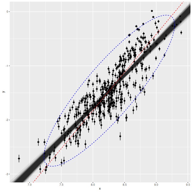
Once again the model seems to fit the data pretty well, the posterior predictive check is reasonable, and Stan didn’t complain. Astronomers are often interested in the “cosmic variance” of various quantities, that is the true amount of unaccounted for variation. If the error estimates in this data set are reasonable the cosmic variance in SFR density is estimated by the parameter σ. The mean estimate of around 0.3 dex is consistent with other estimates in the literature¹see the compilation in the paper by Speagle et al. that I cited last time, for example.

I noticed in preparing the last post that several authors have used something called “orthogonal distance regression” (ODR) to estimate the star forming main sequence relationship. I don’t know much about the technique besides that it’s an errors in variables regression method. There is an R implementation in the package pracma. The red dashed line in the plot above is the estimate for this dataset. The estimated slope (1.41) is much steeper than the range of estimates from this model. On casual visual inspection though it’s not clearly worse at capturing the mean relationship.