Instead of trying a systematic investigation I’m just going to go through each IFU and discuss whatever I found interesting, with no particular theme in mind. I still don’t really know what I’m going to find since it’s been a while since I looked at model results. Besides modeling star formation histories for each spectrum I calculate summaries in the form of posterior marginal means, standard deviations, and a few quantiles for a large number of quantities. Some of these are highly model dependent such as 100 Myr averaged star formation rates and specific star formation. Some are only weakly model dependent, such as emission line fluxes1These depend on correction for absorption, but we don’t need a believable star formation history for that, just a reasonable template match. One thing I haven’t looked at much is stellar metallicities and especially their evolution in the models. There are always contributions from all metallicity bins at all times in my models, and how to interpret them or whether even to try still puzzles me. I am starting to look more seriously at strong emission line metallicity estimates. The estimator proposed by Dopita et al. (2016) based on [N II], [S II], and Hα seems especially promising since they’re usually detected with reasonable precision in SDSS spectra.
So, the plan is to look at each IFU, working my way outward in the disk in the same order as my second post in this series.
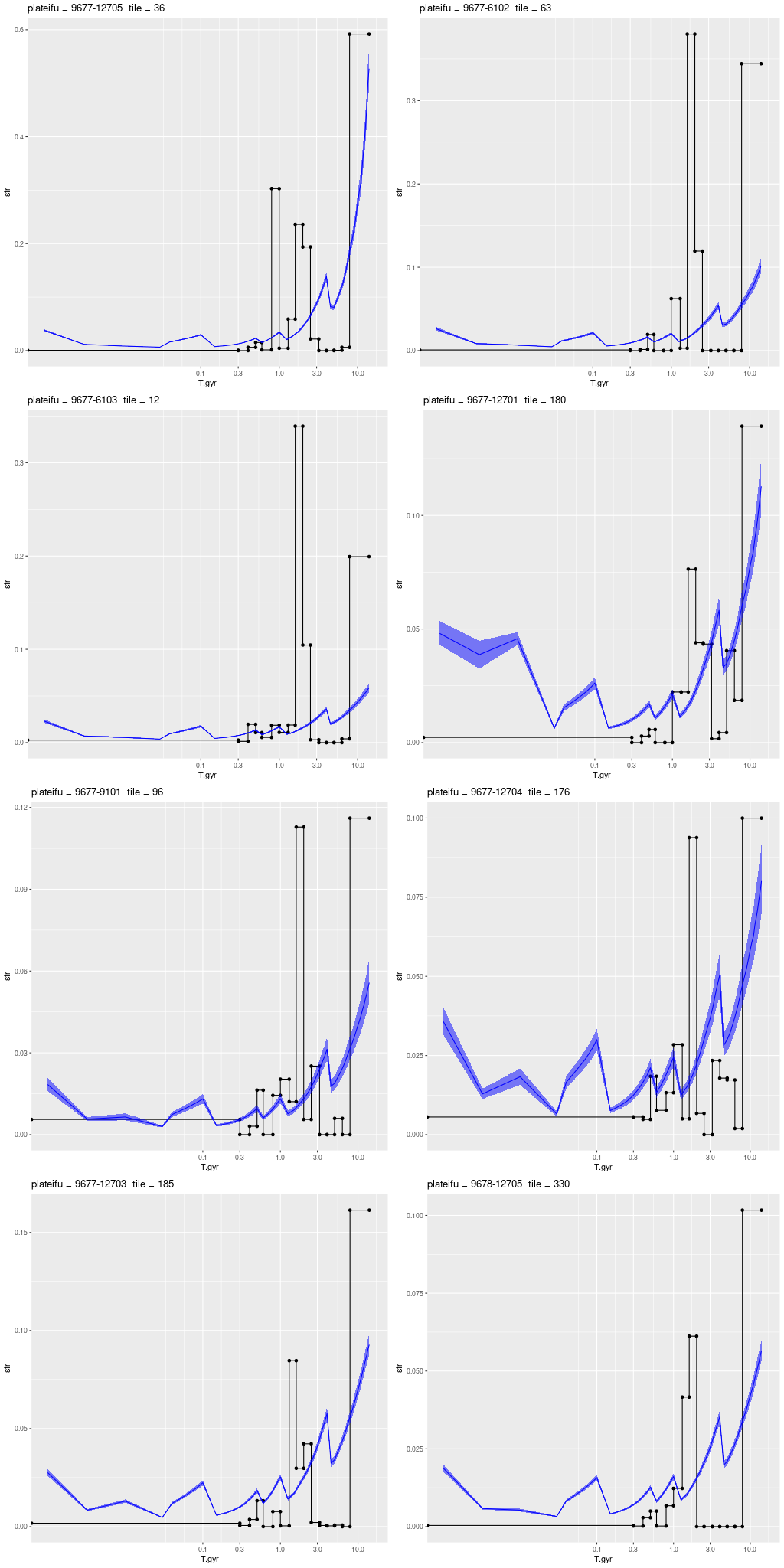
plateifu 9677-12705 (mangaid 52-4)
This is the innermost IFU with a projected distance from the nucleus of 1.9 kpc. According to Walterbos and Kennicutt (1988) the effective radius of the bulge is 2 kpc, so a significant fraction of the light is coming from bulge stars.
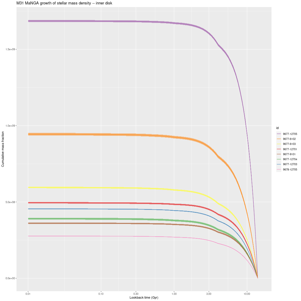
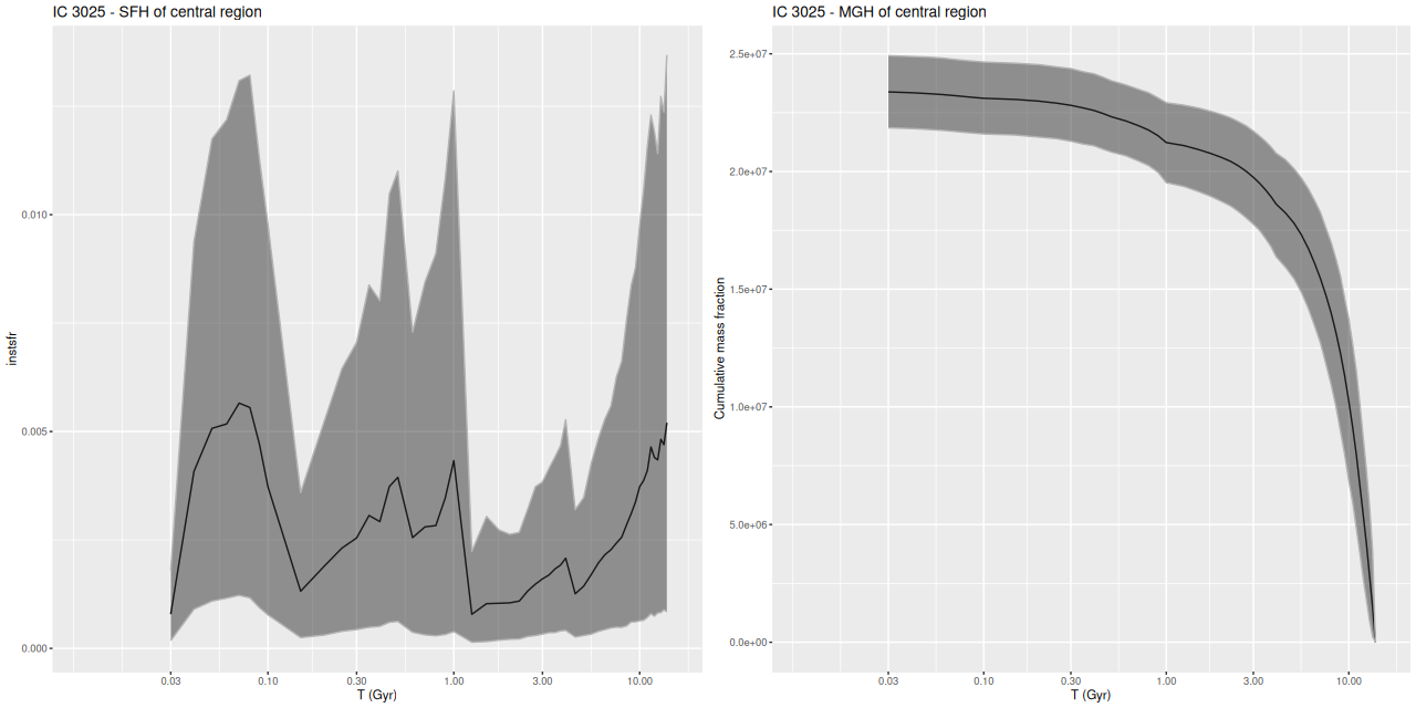
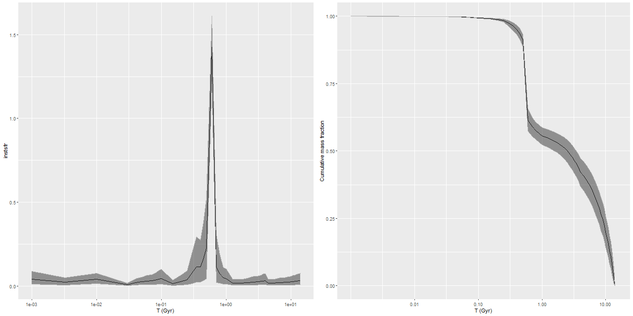
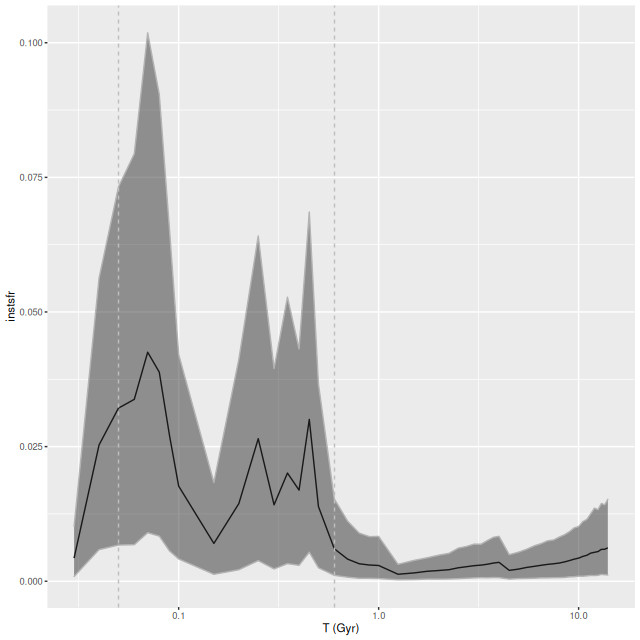
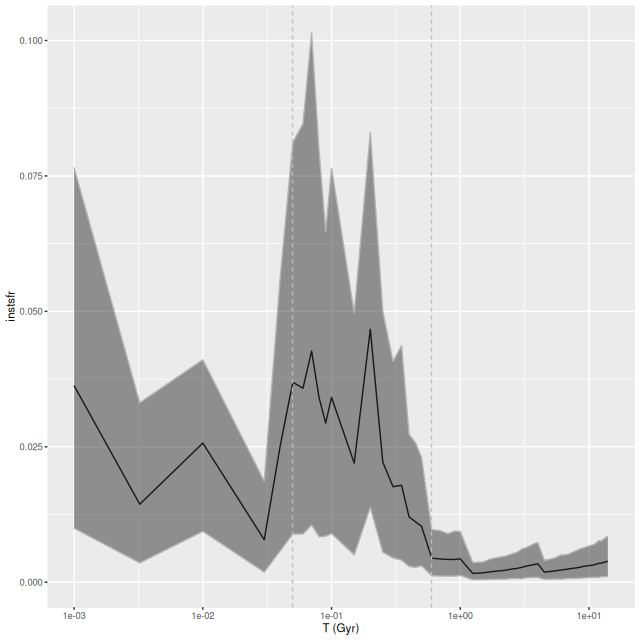
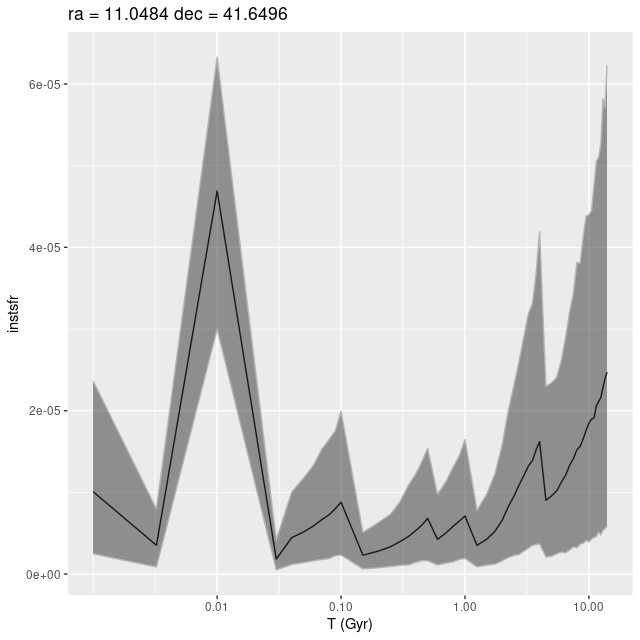
What’s most interesting about this IFU is what it lacks, which is any significant star formation. I also saw little spatial variation in model star formation histories, so I’ll simply repeat the IFU wide history compared to the nearest PHAT tile:
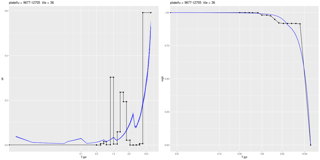
This region had the most rapid initial stellar mass growth and conversely the steepest decline in SFR of any of the MaNGA IFU’s, which is completely consistent with the consensus “inside out” growth paradigm.
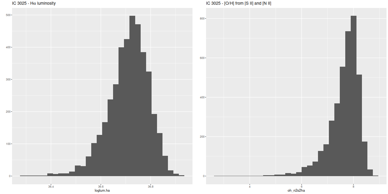
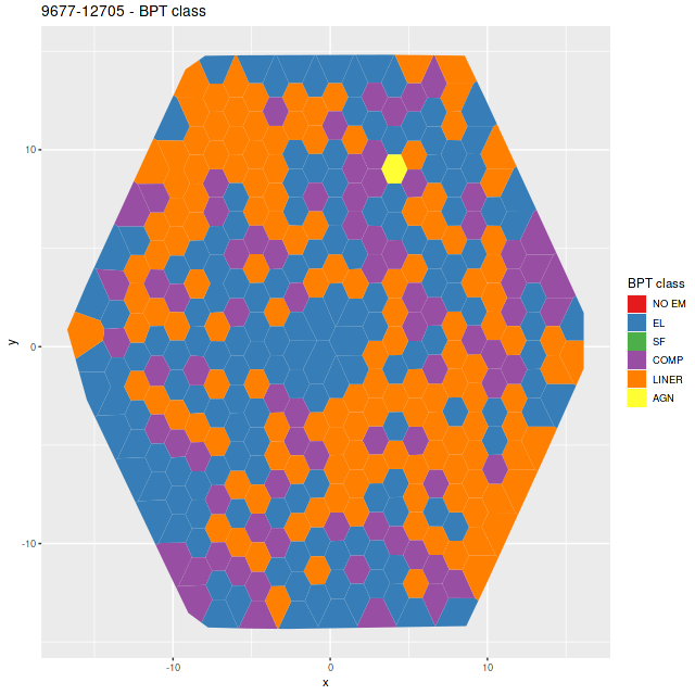
One other moderately interesting result is that despite the lack of young stars there are detectable emission lines throughout with a mix of “LINER” and composite like line ratios from the [N II]/Hα vs. [O III]/Hβ diagnostic and the classification scheme of Kauffmann with Schawinski’s addition of the LINER/AGN divide. As is well known by now LINER (and presumably “composite” although I haven’t seen literature on the issue) emission can be spatially extended and does not at all necessarily indicate ionization by an AGN. M31 has widespread emission from diffuse ionized gas. About 14% of all binned spectra had line ratios in these categories and “AGN” like, and 90% of the LINER-like spectra are in this IFU. A similar fraction of spectra have star forming emission line ratios, which reflects the patchy nature of star formation in M31.
plateifu 9677-6102 (mangaid 52-3)
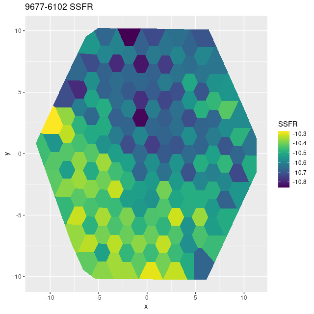
There’s little to say about this one. The entire IFU is offset by a small amount from some GALEX UV bright sources and there are no objects in any of the catalogs I’ve loaded within the footprint. The only prominent feature is a very prominent dust lane that covers the southeastern half of the IFU. Oddly, the estimated specific star formation rate tracks the dust rather closely.
There’s a clear correlation between SSFR and optical depth of attenuation, and also with the “tilt” of the attenuation relation:
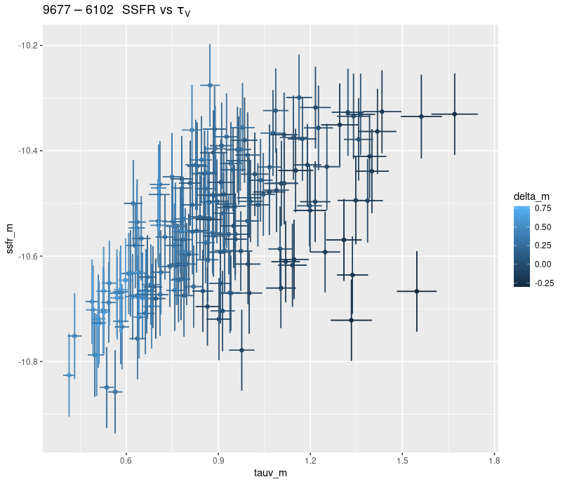
Whether this is meaningful or a modeling artifact I can’t say at this point. I kept my simple single component dust model for these runs even though M31 is known to have both a foreground screen and embedded dust.
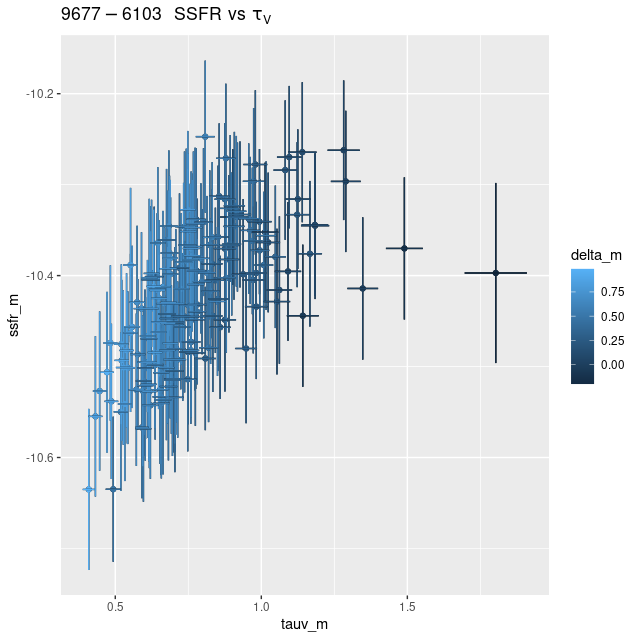
plateifu 9677-6103 (mangaid 52-2)
This again is in a nearly featureless area except for a prominent dust lane, with no sources in any catalog I consulted. The entire IFU lacks significant emission and there is no evidence in the models for significant recent star formation. Oddly, there’s a very similar relation between model specific star formation rate and model optical depth:
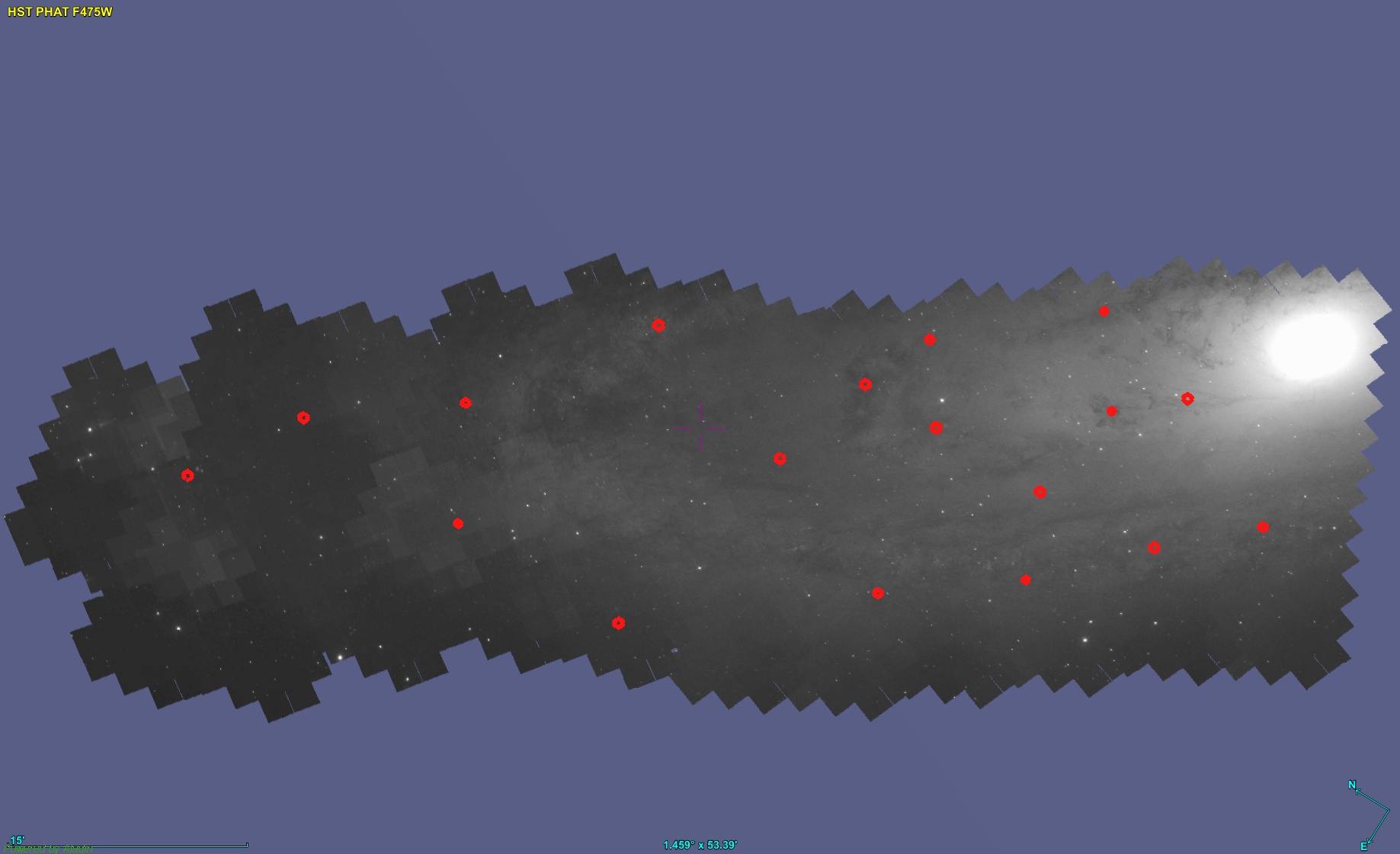
plateifu 9677-12701 (mangaid 52-8)
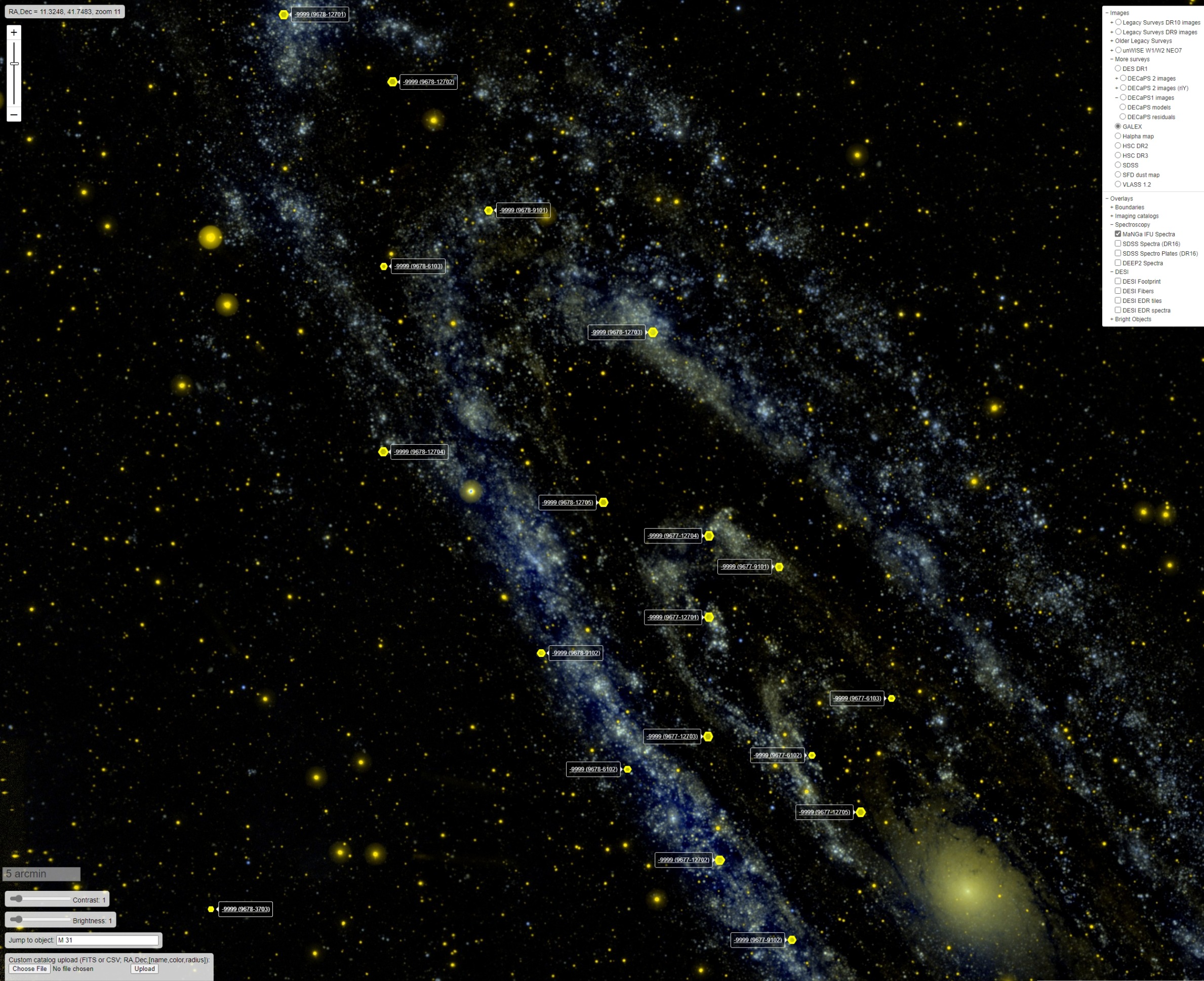
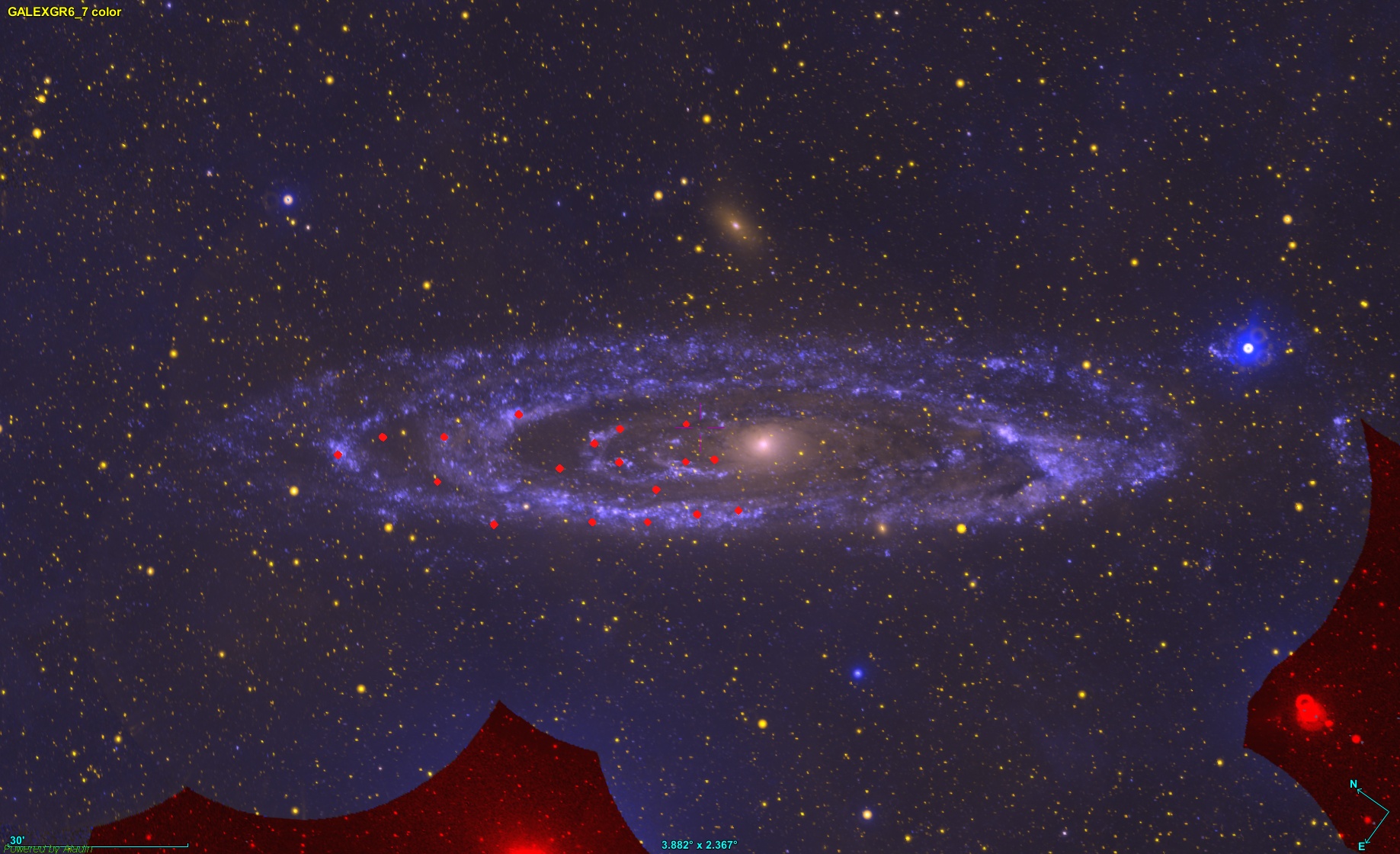
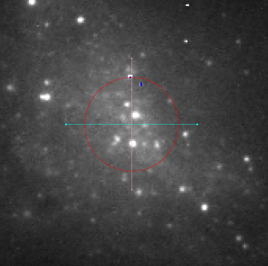
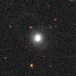
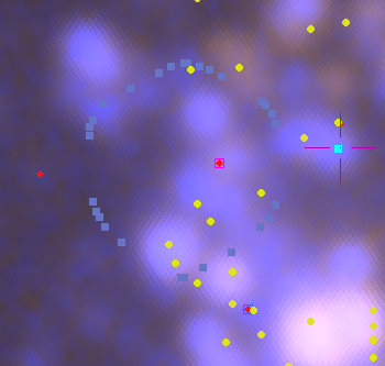
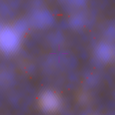
This is the closest IFU to the nucleus that lies within a significant spiral structure as seen by GALEX. The thumbnail below shows its position overlaid on the false color GALEX image available within Aladin. The IFU appears to lie in a spur off a spiral arm a little farther out2There doesn’t seem to be a strong consenus about the overall spiral structure of M31. All modern authors agree that the “10 kpc ring” is a complete ring, with a split in the south not too far from the projected position of M32. I’ve also seen references to 6 and 16 kpc rings, but others claim that various classes of young objects are strung out along a pair of logarithmic spirals. This idea goes back to early 1960’s work by Baade and Arp. I will just note IFU’s in UV bright areas in GALEX since this seems to be the best tracer of recent star formation and a number of discrete UV bright sources are visible within its footprint, which is marked with the irregular set of blue symbols. Also shown are cataloged positions of H II regions (yellow dots), red supergiants (red diamonds), and an OB association (blue square)3data sources are given in the last post. All of these are available through Aladin’s data collection.
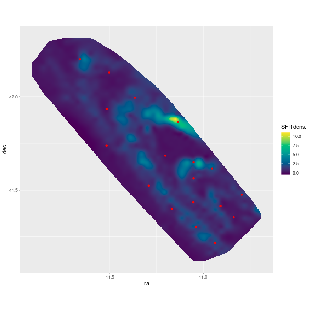
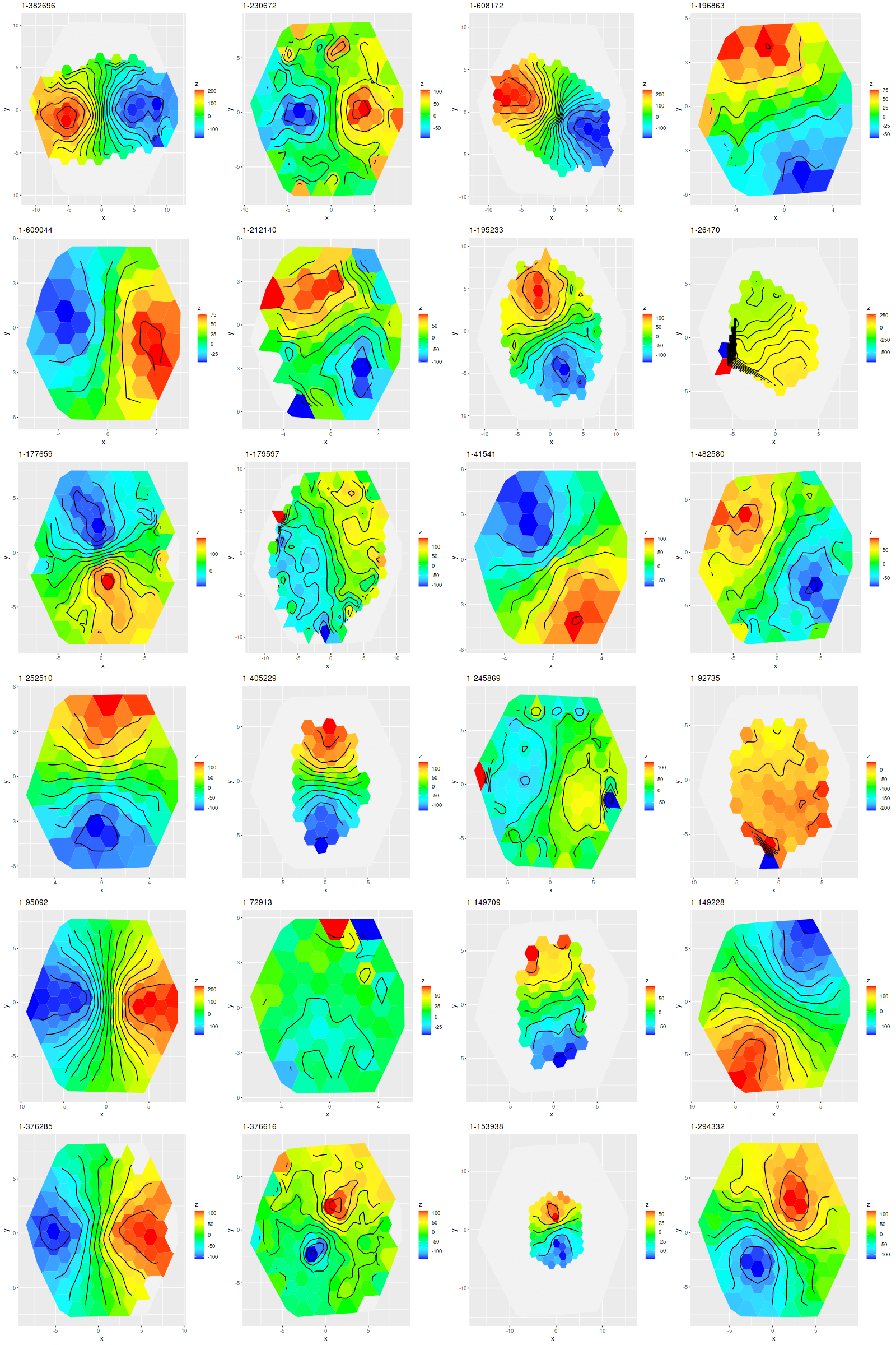
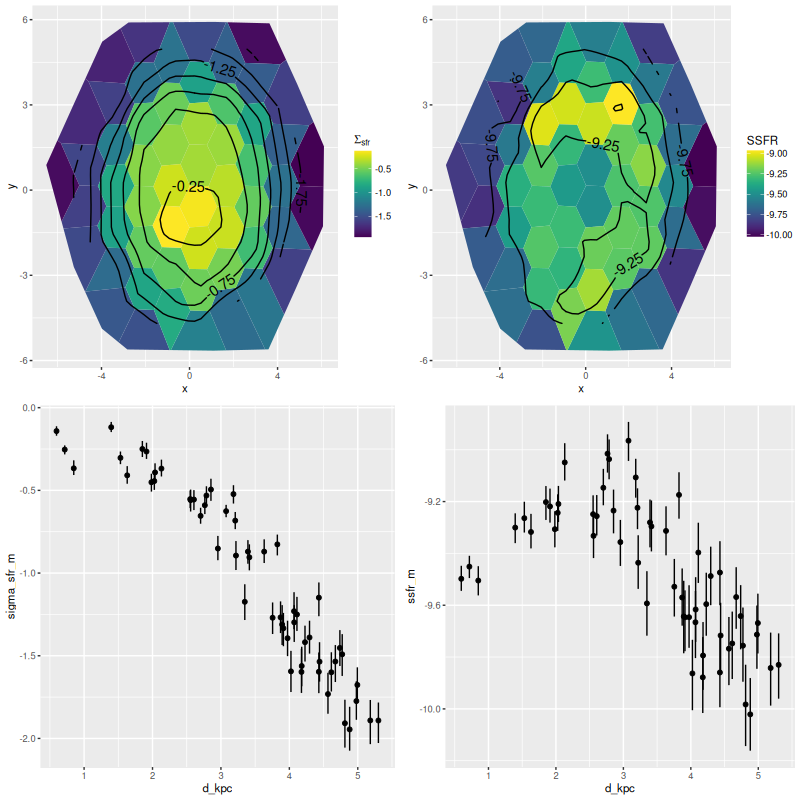
Let’s look at a couple of maps. The blank area at upper right was masked due to a likely foreground star. The spectra in the chain of blank areas at bottom had Hα partially masked. Units in the Hα luminosity density map are log10 ergs/sec/kpc2, uncorrected for attenuation. Units of the SFR density maps are log10 M☉/yr/kpc2.
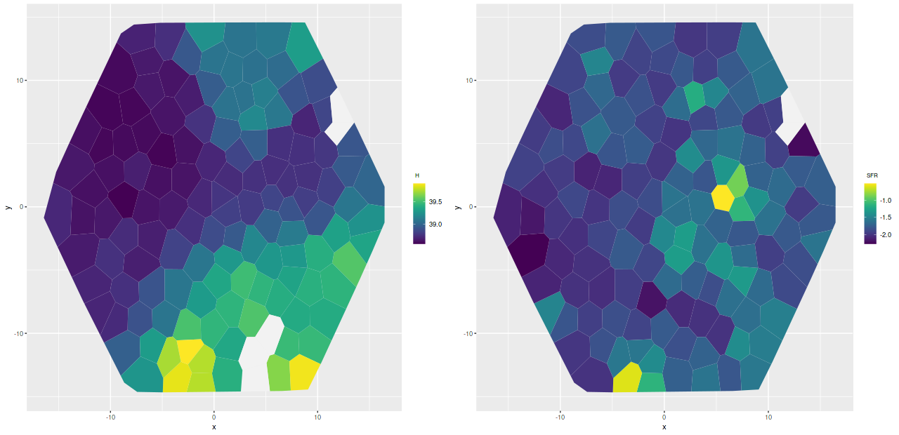
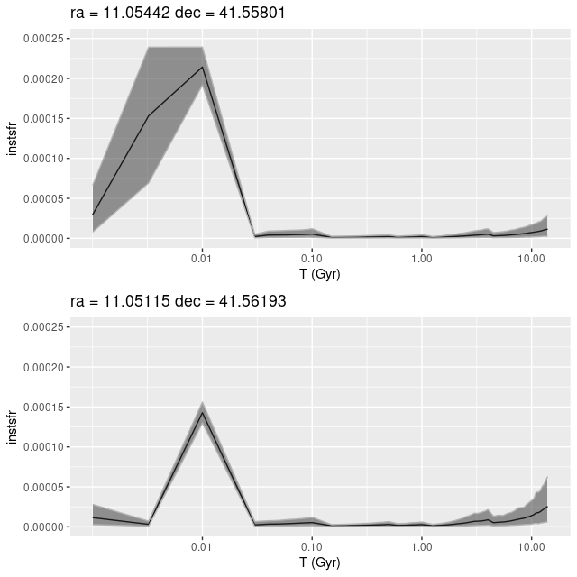
To a pretty good approximation regions that are relatively bright in Hα track the UV bright areas and cataloged H II regions. There are two areas that stand out as having much higher than average SFR density. One, at lower left, coincides with a bright H II region. The other one, at center right, has low Hα luminosity but lies right on the cataloged position of a red supergiant. The presence of an evolved star and absence of emission suggests that star formation has recently (in the last ~70 Myr, say) ended in that area. Comparing the model star formation histories the region with little Hα emission does show a sharp drop-off after a peak at 10 Myr lookback time:
One other thing I’ll just note for now is that regions with the highest star formation rate tend to have neighboring regions with higher than average star formation as well. These seem to occur in clumps or chains a few 10s of parsec in size. I will get, eventually, to some more dramatic examples.
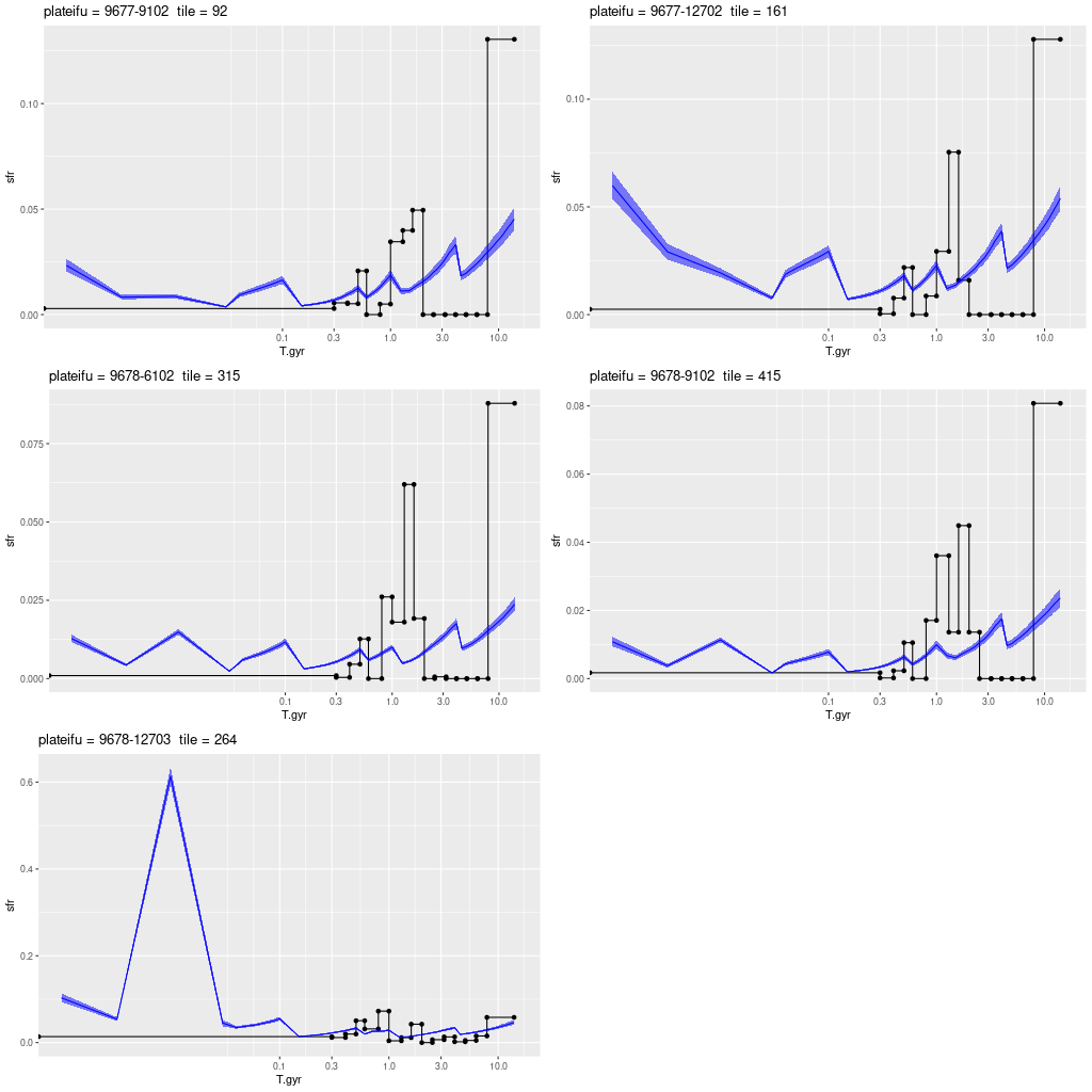
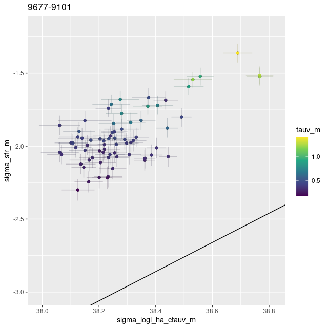
plateifu 9677-9101 (mangaid 52-9)
This and the next IFU are in a spiral segment that some authors call the “6 kpc ring,” but the GALEX false color image shows no very bright UV sources and there are no cataloged young objects within the footprint.
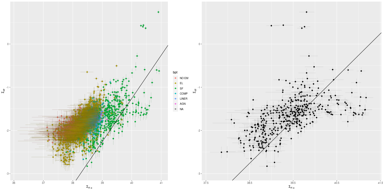
One mildly interesting result is that the modeled 100 Myr SFR density correlates rather strongly with Hα luminosity density, but an order of magnitude higher than predicted from Calzetti’s calibration. All of the emission in this region appears to be from diffuse ionized gas as there are no cataloged discrete sources of emission, and no regions with starforming line ratios. A literal interpretation of this, which might even be true, is that star formation has ceased in the recent past.
plateifu 9677-12704 (mangaid 52-5)
This is also in the 6 kpc spiral feature but in an area with no bright UV sources and that appears to be heavily dust obscured in optical images. Since I don’t have anything very interesting to say about this region I’ll just post the modeled star formation history for the region within the IFU footprint with the highest modeled SFR density. This is near the western edge of the IFU and isn’t associated with any cataloged young objects.
The region with the highest Hα luminosity is near the southwest edge and covers the position of a cataloged planetary nebula. The emission line ratios are inconsistent with a starforming region, falling in Kauffmann’s “AGN” region.
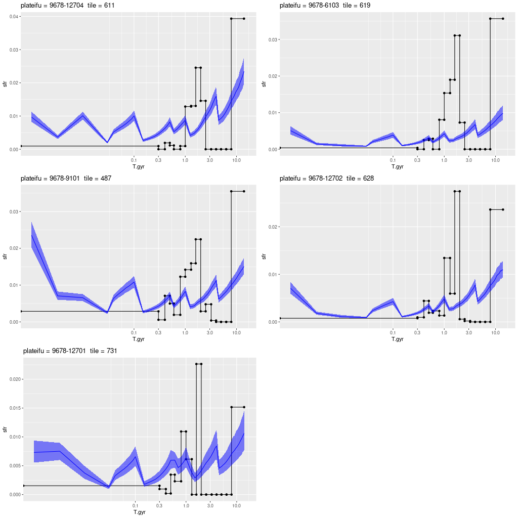
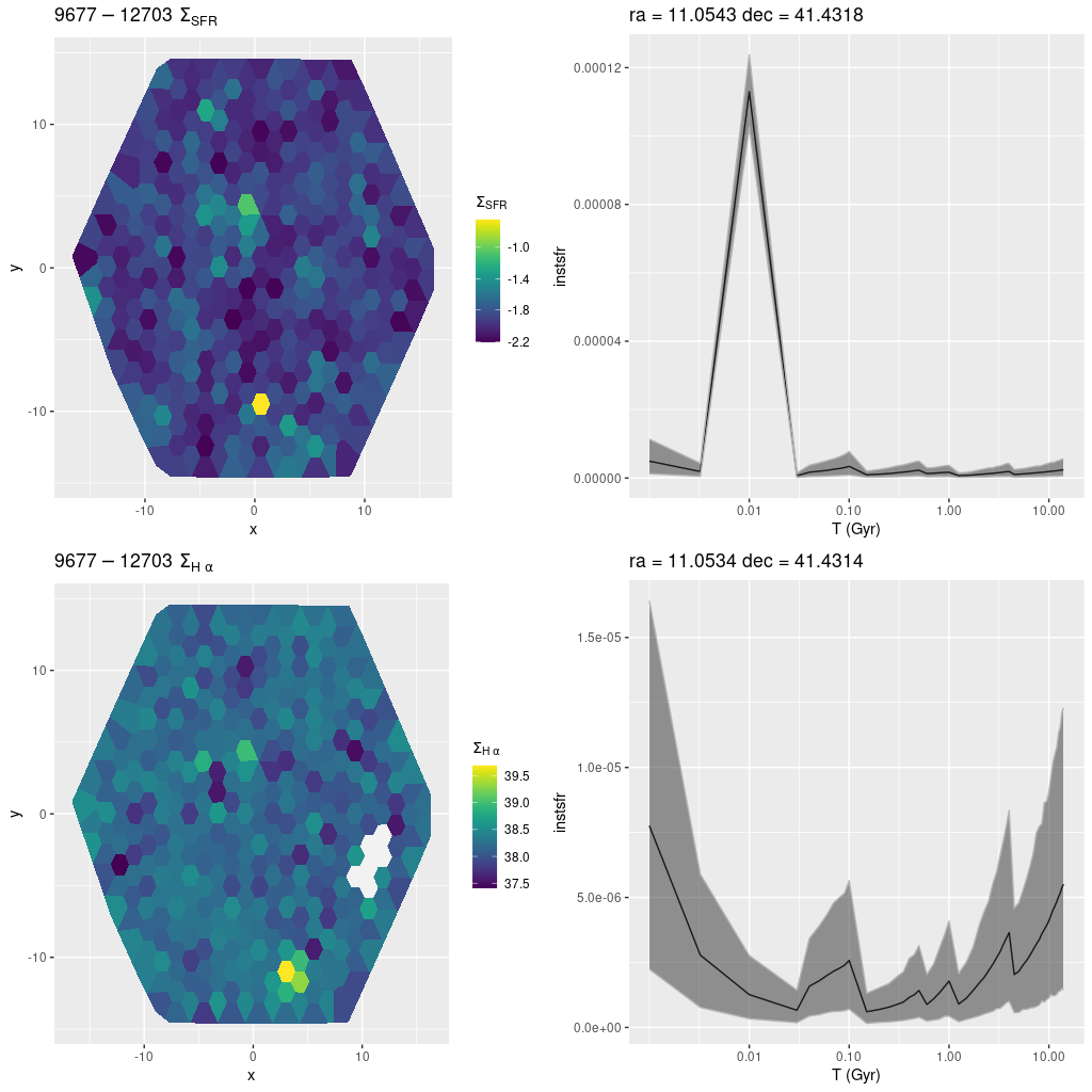
plateifu 9677-12703 (mangaid 52-6)
This and the last IFU are in an inter-line region between the 6 and 10 kpc structures as seen by GALEX, but with lots of diffuse starlight and relatively little dust. Emission lines are weak or undetected throughout, but there is a cataloged H II region near the southern edge. The peak in Hα luminosity density is easily seen in the map below in the bottom left pane. The region with the highest SFR density is displaced by ~10 pc. from the region with highest Hα luminosity. Interestingly, the SFR models show significant differences in recent histories: the region with highest SFR shows a very sharp and short lived peak at ~10 Myr, while the highest Hα luminosity region is still growing in SFR (per the model). Again, I hesitate to take these model histories too literally, especially at the youngest ages, but these are consistent with the fact that ionized gas emission will fade rather rapidly as the most massive stars in a region evolve away from the main sequence.
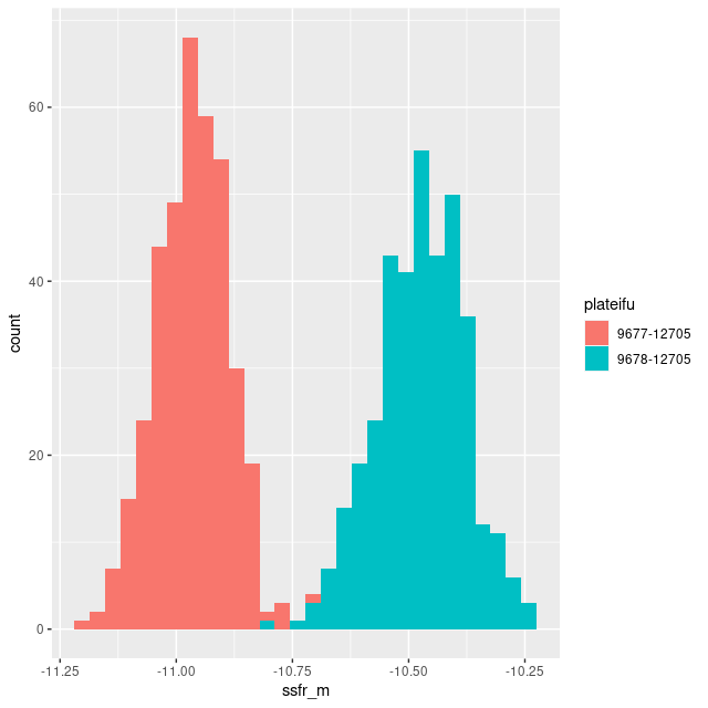
plateifu 9678-12705 (mangaid 52-21)
I don’t have much to say about this one either. It lies in a region that’s almost completely blank in the GALEX imaging, with a rather uniform sprinkle of stars in PHAT and the DSS2 image displayable in Aladin. Ionized gas emission is weak or undetected throughout. For the sake of having a graph to display here is a histogram of the per spectrum mean specific star formation rate (100 Myr average as always) comparing this IFU to the innermost one — plateifu 9677-12705.
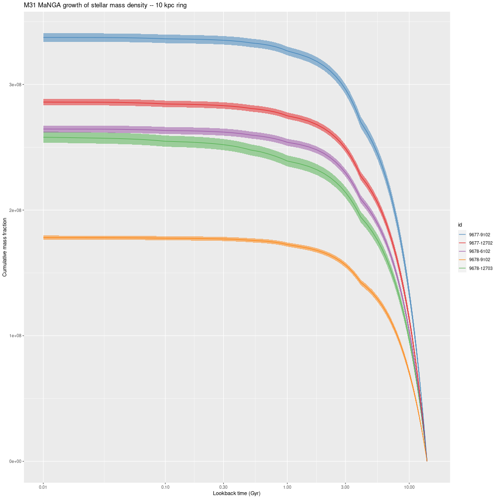
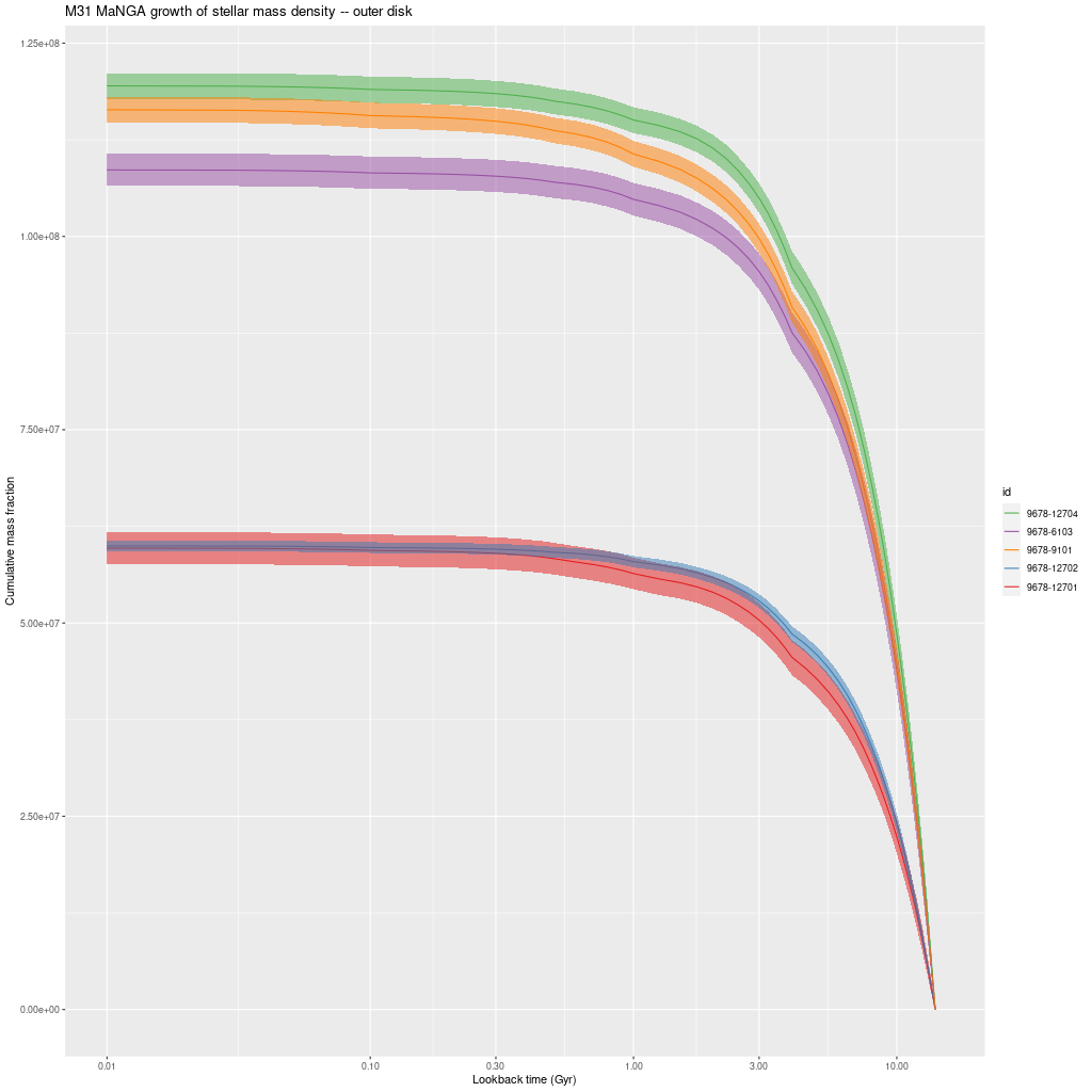
I hope to finish off M31 in one or at most two more posts. Next up are IFUs that fall in or near the 10 kpc ring, followed by the outer disk.