
In the last post I showed that the posterior distribution of the model parameters as estimated by Stan look rather different than the distribution of maximum likelihood estimates under repeated realizations of the noisy “observation” vector, but I didn’t really discuss why they look different. For starters it’s not because the Stan model failed to converge, nor is there any evidence for missed multimodality in the posterior. Although Stan threw some warnings for this model run they involved fewer than 1% of the post-warmup iterations and there was no sign of pathological behavior (by the way I recommend the package shinystan for a holistic look at Stan model outputs). Multimodality can happen — often it manifests as one or more chains converging to different distributions than the others, but sometimes Stan can fail to find extra modes. But I haven’t seen any evidence for this in repeated runs of this and similar models, nor for that matter in real data SFH modeling.I mentioned that I copied the prior over from my real data models and this is probably not quite what I wanted to use, and that gets us into the topic of investigating the effect of the prior in shaping the posterior. That’s not what caused the difference either, but I’ll look at it anyway.
The real reason I think is one that I still find paradoxical or at least sorta counterintuitive. The main task of computational Bayesian inference is to explore the “typical set” (a concept borrowed from information theory). There’s a nice case study by one of Stan’s principal developers showing through geometric arguments and some simple simulations that the typical set can be, and usually is, far (in the sense of Euclidean distance) from the most likely value and the distance increases with increasing dimensionality of the parameter space. We can show directly that is happening here.
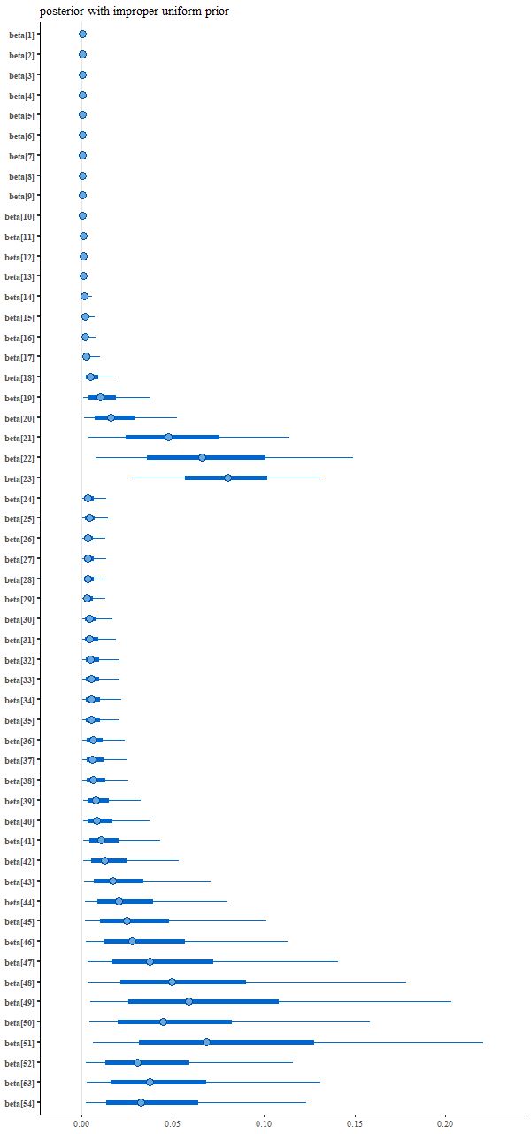
Let’s first modify the model to adopt an improper uniform prior on the positive orthant, which just requires removing a line from the model block of the Stan code (if no prior is specified it is implicitly made uniform, which in this case is improper):
parameters {
  vector<lower=0.>[M] beta;
}
model {
  y ~ normal(X * beta, sdev);
}
Modern Bayesians usually recommend against the use of improper priors, but since the likelihood in this model is Gaussian the posterior is proper. The virtue of this model is the maximum a posteriori (MAP) solution is also the maximum likelihood solution. Stan can do general nonlinear optimization as well as sampling, using by the way conventional gradient based algorithms rather than Monte Carlo optimization.
First, I run the sampler on this model, and extract the posterior:
sfit0 <- stan(file="simplenn0.stan",data=stan_dat,iter=1000,warmup=500,open_progress=T,control=list(max_treedepth=13))
post0 <- extract(sfit0)
smod0 <- stan_model("simplenn0.stan")
I do this to get a starting guess for the optimizer and because we’ll do some comparisons later. For some reason rstan’s optimization function requires as input a stanmodel object rather than a file name, so we call stan_model() to get one. Then I call the optimizer, adjusting a few parameters to try to get to a better solution than with defaults:
sopt0 <- optimizing(smod0, data=stan_dat, init=list(beta=colMeans(post0a$beta)), tol_grad=1e-10,tol_rel_obj=1e2,tol_rel_grad=1e4)This completes successfully in a few seconds and returns a reasonable approximation to the solution given by nnls:
> print(sopt0$par[1:54], digits=3)
 beta[1]  beta[2]  beta[3]  beta[4]  beta[5]  beta[6]  beta[7]  beta[8]
6.32e-06 1.57e-05 1.78e-05 1.74e-05 1.66e-05 1.70e-05 1.85e-05 1.66e-05
 beta[9] beta[10] beta[11] beta[12] beta[13] beta[14] beta[15] beta[16]
1.90e-05 2.86e-05 3.91e-05 5.09e-05 7.34e-05 1.63e-04 2.45e-04 2.69e-04
beta[17] beta[18] beta[19] beta[20] beta[21] beta[22] beta[23] beta[24]
5.86e-04 4.52e-03 1.67e-02 3.54e-03 8.83e-09 2.58e-01 4.61e-04 2.01e-04
beta[25] beta[26] beta[27] beta[28] beta[29] beta[30] beta[31] beta[32]
2.11e-04 1.69e-04 1.53e-04 1.61e-04 1.43e-04 2.17e-04 2.70e-04 2.98e-04
beta[33] beta[34] beta[35] beta[36] beta[37] beta[38] beta[39] beta[40]
3.35e-04 3.51e-04 3.34e-04 4.45e-04 4.77e-04 5.68e-04 7.26e-04 8.77e-04
beta[41] beta[42] beta[43] beta[44] beta[45] beta[46] beta[47] beta[48]
9.38e-04 1.36e-03 2.01e-03 9.84e-04 5.63e-04 3.65e-04 2.98e-04 1.79e-03
beta[49] beta[50] beta[51] beta[52] beta[53] beta[54]
6.99e-01 1.52e-04 1.10e-05 1.81e-03 2.73e-04 3.31e-04
> print(nnfit.1$x, digits=3)
 [1] 0.000262 0.000000 0.000000 0.000000 0.000000 0.000000 0.000000 0.000000
 [9] 0.000000 0.000000 0.000000 0.000000 0.000000 0.003887 0.000000 0.000000
[17] 0.000000 0.000000 0.000000 0.025777 0.000000 0.258491 0.000000 0.000000
[25] 0.000000 0.000000 0.000000 0.000000 0.000000 0.000000 0.000000 0.000000
[33] 0.000000 0.000000 0.000000 0.000000 0.000000 0.000000 0.000000 0.000000
[41] 0.000000 0.000000 0.000000 0.000000 0.000000 0.000000 0.000000 0.000000
[49] 0.673700 0.000000 0.000000 0.000000 0.035233 0.003006
> sopt0$par["ll"]
      ll
14986.16
> ll.1
[1] 14986.43
>
Now let’s use these to initialize the chains for another Stan model run (I also adjusted some of the control parameters to get rid of warnings from the first run):
> inits <- lapply(X=1:4,function(X) list(beta=sopt0$par[1:54]))
> sfit0a <- stan("simplenn0.stan",data=stan_dat,init=inits,iter=1000,warmup=500,open_progress=T,control=list(max_treedepth=14,adapt_delta=0.9))
Now examine trace plots for the first few warmup draws for a few parameters. The top rows trace the first 100 warmup iterations. The right 4 are initialized with the approximate maximum likelihood solution, the left are from the first randomly initialized run. The ML initialized chains quickly move away from that point and reach stationary, well mixed distributions in just a few iterations. The randomly initialized chains take slightly longer to get to the same stationary distributions.
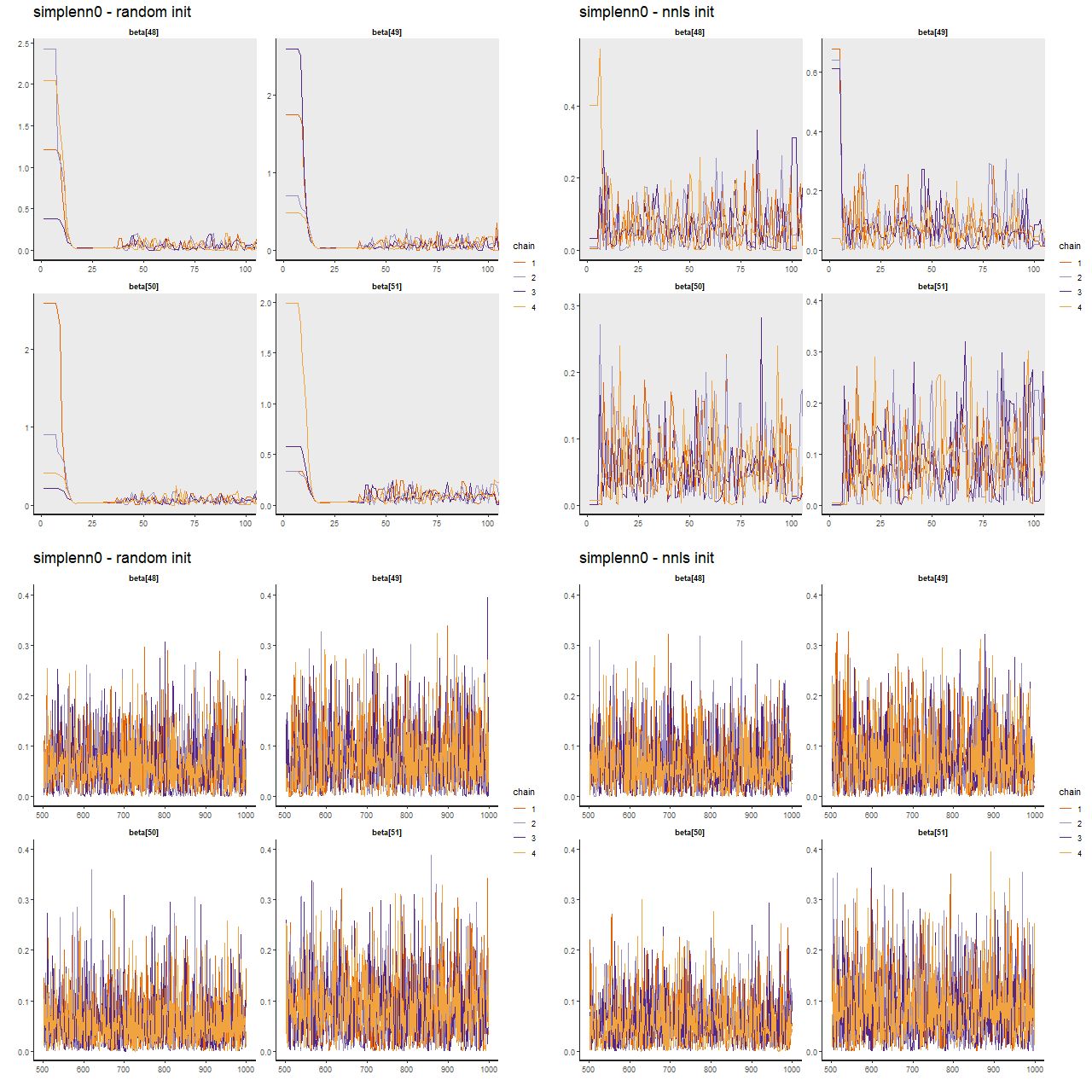
(TL) warmup iterations with random inits
(TR) warmup iterations with nnls solution inits
(BL) post-warmup with random inits
(BR) post-warmup with nnls solution inits
And the resulting interval plot for the model coefficients isn’t noticeably different from the first run:
Nowadays Bayesians generally advise using proper priors that reflect available domain knowledge. I had done that originally but without thinking that the prior wasn’t quite right given the data manipulations that I had performed. A better prior that incorporates “domain” knowledge without being too specific might be something like a truncated normal with the same scale parameter for each coefficient, which in this case can reasonably be set to 1. That’s accomplished by adding back just one line to the model block:
model {
  beta ~ normal(0, 1.);
  y ~ normal(X * beta, sdev);
}
which leads to the following posterior interval plot compared to the original:
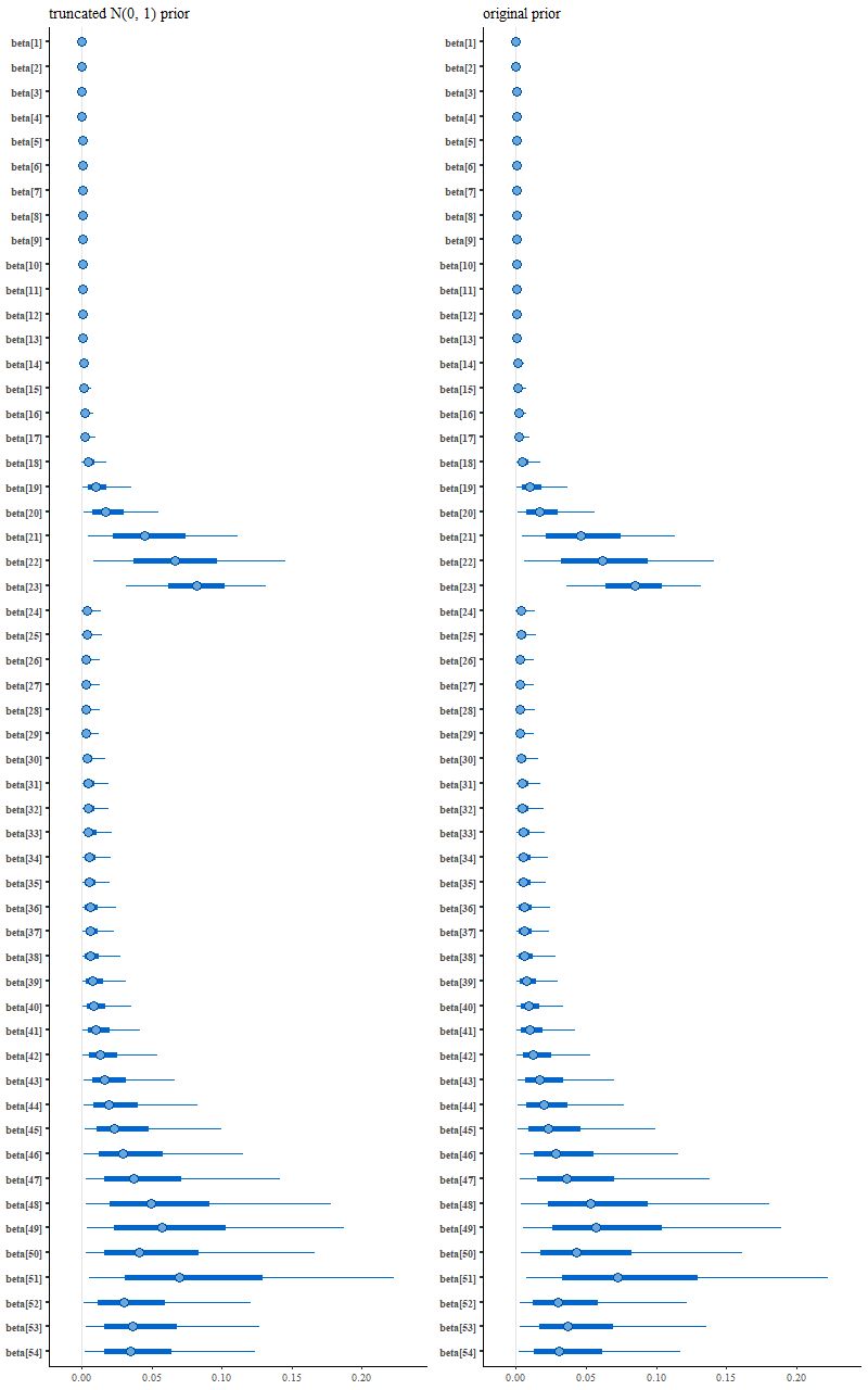
(R) original variable width prior
See the difference? Close inspection will show some minor ones, but it’s not immediately clear if they’re larger than expected from sampling variations.
Can we induce sparsity?
Here are a couple ideas I thought might work but didn’t. One way to induce sparsity in regression models is called the lasso, or more technically L-1 penalized regression. This is just least squares with an added penalty proportional to the absolute values of the model parameters. A more or less equivalent idea in Bayesian statistics is to add a double exponential or Laplacian prior. Since the parameters here are non-negative we can use an exponential prior instead.
Yet another possible prior inspired by “domain knowledge” is to notice that the coefficient values I picked sum to 1. A sum to 1 constraint can be programmed in Stan by declaring the parameter vector to be a simplex. Leaving out an explicit prior will give the parameters implicitly uniform priors.
parameters {
  simplex[M] beta;
}
model {
  y ~ normal(X * beta, sdev);
}
Interestingly enough for possible future reference this model ran much faster than the others and threw no warnings, but it didn’t produce a sparse solution:
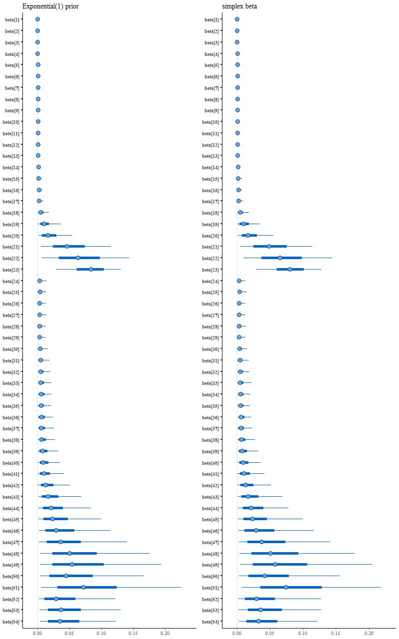
(L) exponential prior
(R) unit simplex parameter vector
Back to the drawing board and with a bit of web research it turns out there is a fairly standard sparsity inducing prior known as the “horseshoe” described in yet another Stan case study by another principal developer, Michael Betancourt. The parameter and model block for this looks like
parameters {
  vector<lower=0.>[M] beta;
  real<lower=0.> tau;
  vector<lower=0.>[M] lambda;
}
model {
  tau ~ cauchy(0, 0.05);
  lambda ~ cauchy(0, 1.);
  beta ~ normal(0, tau*lambda);
  y ~ normal(X * beta, sdev);
}
This is the “classical” horseshoe rather than the preferred prior that Betancourt refers to as the “Finnish horseshoe.” This took some fiddling with hyperparameter values to produce something sensible that appeared to converge, but it did indeed produce a sparse posterior:
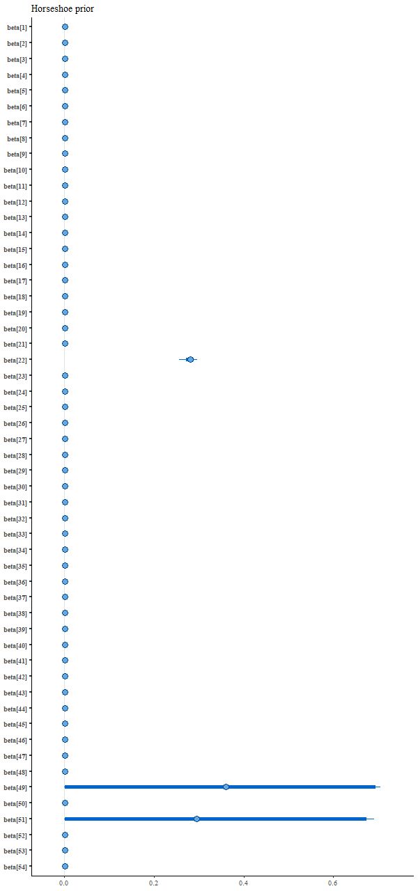
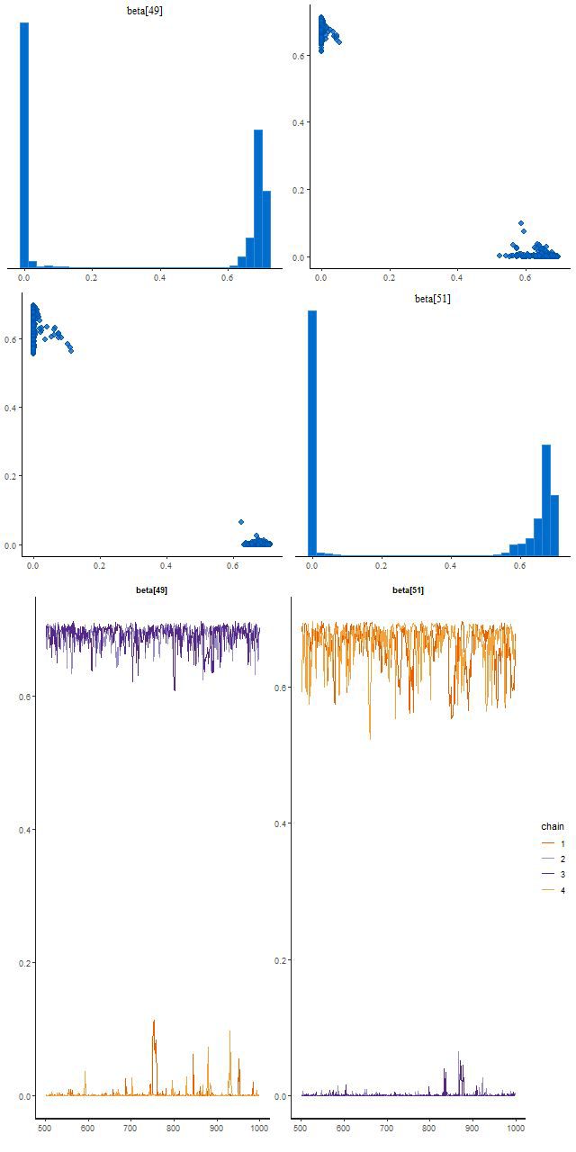
This run did find two posterior modes, and this illustrates the typical Stan behavior I mentioned at the beginning of this post. Two chains found a mode where beta[49] is large and beta[51] near 0, and two found one with the values reversed. There’s no jumping between modes within a chain:
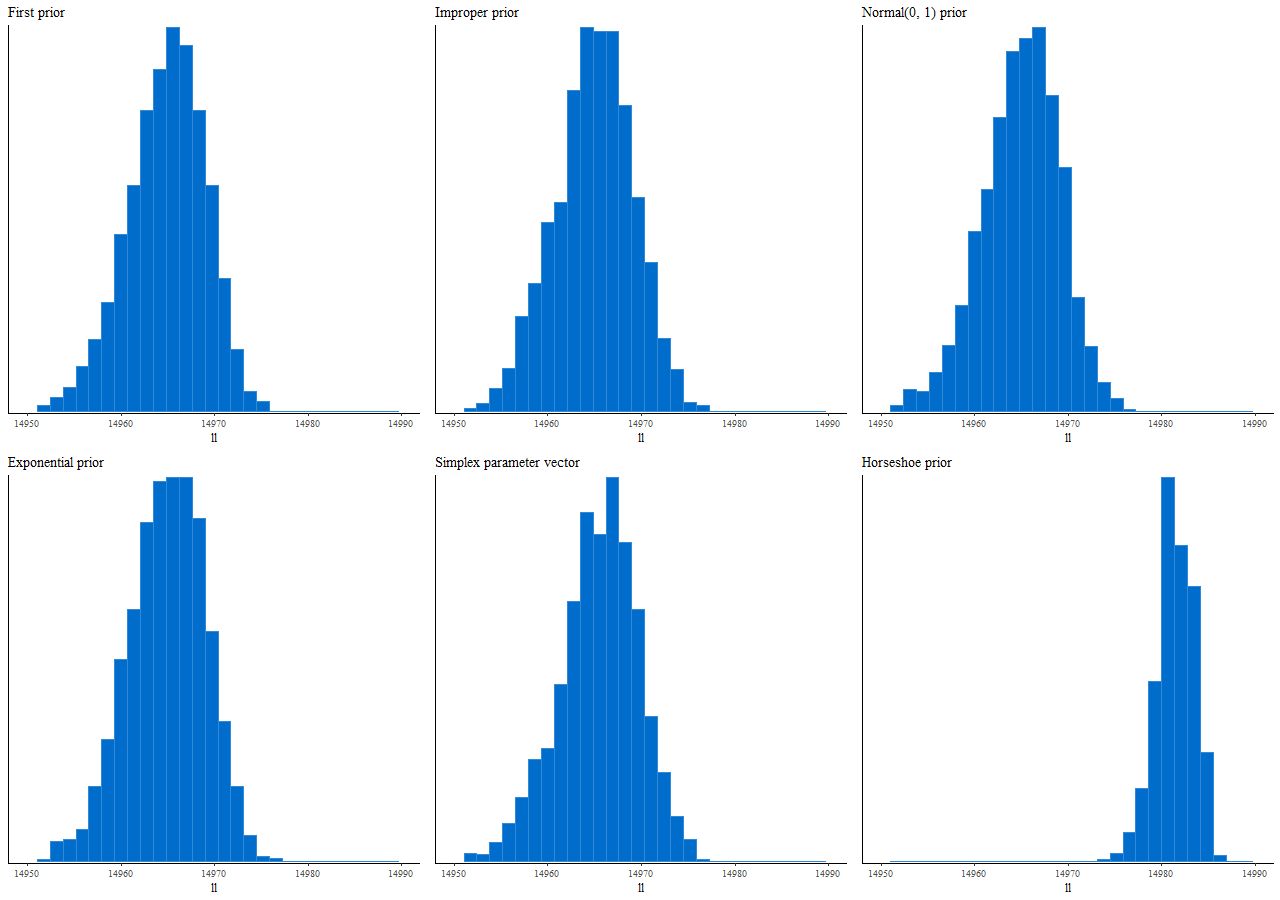
Finally, here are the distributions of log-likelihood for the 6 priors considered in the last two posts:
Should we care about sparsity? In statistics and machine learning sparsity is usually considered a virtue because one often has a great many potential predictors, only a few of which are thought to have any real predictive value. In star formation history modeling on the other hand astronomers usually think of star formation as varying relatively smoothly over time, at least when averaged over galactic scales. Star formation occurring in a few discrete bursts widely separated over cosmic history seems unphysical, which makes interpreting (or for that matter believing) the results challenging.
One takeaway from this exercise is that in a data rich environment the details of the prior don’t matter too much provided it’s reasonable, which in the context of star formation history modeling specifically excludes one that induces sparsity — despite the fact that in this contrived example the sparsity inducing prior recovers the inputs accurately while generic priors do not. Of course maximum likelihood estimation does even better at recovering the inputs with far less computational expense.
Coming soon, I hope, back to real data.