
In the course of studying star formation histories I’ve accumulated lots of velocity fields similar to the ones I just posted about. For purposes of SFH modeling their only use is to reduce wavelengths to the galaxy rest frame. It’s not sufficient just to use the system redshift because peculiar velocities of a few hundred km/sec (typical for disk galaxies) translate into spectral shifts of 2-3 pixels, enough to seriously impair spectral fits. Naturally however I wanted to do something else with these data, so I decided to see if I could model rotation curves. And, since I’m interested in Bayesian statistics and was using it anyway, I decided to try Stan as a modeling tool. This is hardly a new idea; in fact I was motivated in part by a paper I encountered on arxiv by Oh et al. (2018), who attempt a more general version of essentially the same model.
The basic idea behind these models is that if the stars and/or gas are confined to a thin disk and moving in its plane we can recover their full velocities from the measured radial velocities when the plane of the galaxy is tilted by a moderate amount to our line of sight (inclination angles between about 20o and 70o are generally considered suitable). The equations describing the tilted disk model are given in, among many other places, Teuben (2002). I reproduce them here with some minor notational changes. The crude sketch below might or might not make the geometry of this a little clearer. The galaxy is inclined to our line of sight by some angle \(i\) (where 0 is face-on), with the position angle of the receding side \(\phi\), by convention measured counterclockwise from north. The observed radial velocity \(v(x,y)\) at cartesian coordinates \((x,y)\) in the plane of the sky can be written in terms of polar coordinates \((r, \theta)\) in the plane of the galaxy as
$$v(x,y) = v_{sys} + \sin i (v_{rot} \cos \theta + v_{exp} \sin \theta) $$
where
$$\sin \theta = \frac{- (x-x_c) \cos \phi – (y-y_c) \sin \phi}{r \cos i}$$
$$\cos \theta = \frac{ – (x-x_c) \sin \phi + (y-y_c) \cos \phi}{r}$$
and \(v_{sys}, v_{rot}, v_{exp}\) the overall system velocity at the kinematic center \((x_c, y_c)\), rotational (or transverse), and expansion (or radial) components of the measured line of sight velocity.
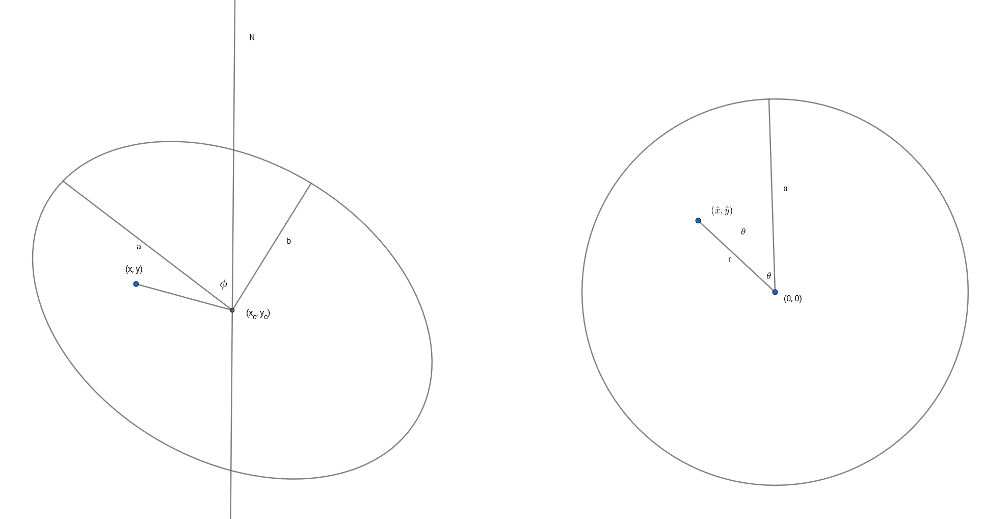
The transformation between coordinates on the sky and coordinates in the plane of the galaxy can be written as a sequence of vector and matrix operations consisting of a translation, rotation, and a stretch:
$$[\hat x, \hat y] = [(x – x_c), (y-y_c)] \mathbf{R S}$$
$$ \mathbf{R} = \left( \begin{array}{c} -\cos \phi & -\sin \phi \\ -\sin \phi & \cos \phi \end{array} \right)$$
$$ \mathbf{S} = \left( \begin{array}{c} 1/\cos i & 0\\ 0 & 1 \end{array} \right)$$
and now the first equation above relating the measured line of sight velocity to velocity components in the disk can be rewritten as
$$v(x, y) = v_{sys} + \sin i [v_{rot}(\hat x, \hat y) \hat y/r + v_{exp}(\hat x, \hat y) \hat x/r]$$
Note that I am defining, somewhat confusingly,
$$\cos \theta = \hat y/r \\ \sin \theta = \hat x/r$$
with
$$r = \sqrt{\hat x^2 + \hat y^2}$$
This is just to preserve the usual convention that the Y axis points up, while also preserving the astronomer’s convention that angles are measured counterclockwise from north.
Stan supports a full complement of matrix operations and it turns out to be slightly more efficient to code these coordinate transformations as matrix multiplications, even though it involves some copying between different data types.
So far this is just geometry. What gives the model physical content is that both \(v_{rot}\) and \(v_{exp}\) are assumed to be strictly axisymmetric. This seems like a very strong assumption, but these can be seen as just the lowest order modes of a Fourier expansion of the velocity field. There’s no reason in principle why higher order Fourier terms can’t be incorporated into the model. The appropriateness of this first order model rests on whether it fits the data and its physical interpretability.
How to represent the velocities posed, and continues to pose, a challenge. Smoothing splines have desirable flexibility and there’s even a lengthy case study showing how to implement them in Stan. I tried to adapt that code and found it to be quite intractable, the problem being that coordinates in the disk frame are parameters, not data, so the spline basis has to be rebuilt at each iteration of the sampler.
In order to get started then I just chose a polynomial representation. This isn’t a great choice in general because different orders of the polynomial will be correlated which leads to correlated coefficient estimates. If the polynomial order chosen is too high the matrix of predictors becomes ill conditioned and data can be overfit. This is true for both traditional least squares and Bayesian methods. The minimum order to be included is linear, because both \(v_{rot}\) and \(v_{exp}\) have limiting values of 0 at radius 0. This is both because of continuity and identifiability: a non-zero velocity at 0 is captured in the scalar parameter \(v_{sys}\). It takes at least a 3rd order polynomial to represent the typical shape of a rotation curve; I found that convergence issues started to become a problem at as low as 4th order, so I just picked 3rd order for the models reported here. In the next or a later post I will show a partial solution to a more flexible representation, and I may revisit this topic in the future.
There are two angles in the model, and this presents lots of interesting complications. First, it’s reasonable to ask if these should be treated as data or parameters of the model. There are useful proxies for both in the photometric data provided in the MaNGA catalog, in fact there are several. Some studies do in fact fix their values. I think this is both a conceptual and practical error. First, these are photometric measurements not kinematic ones. They aren’t the same thing. Second, they are subject to uncertainty, possibly a considerable amount. Failing to account for that could lead to seriously underestimated uncertainties in the velocities. In fact I think much of the literature is significantly overoptimistic about how well constrained are rotation velocities.
So, both the inclination and major axis orientation are parameters. And this immediately creates other issues. Hamiltonian Monte Carlo requires gradient evaluation, and the version implemented in Stan requires the gradient to exist everywhere in \(\mathbb{R}^N\). Bounded parameters are automatically transformed to create new, unbounded ones. But this creates an acknowledged problem that circles can’t be mapped to the real line, at least in a way that preserves probability measure everywhere. There are a couple potential ways to avoid this problem, and I chose different ones for the inclination and orientation angles.
The inclination turned out to be the easier to deal with, at least in terms of model specification. First, the inclination angle is constrained to be between 0 and 90o. Instead of the angle itself I make the parameter \(\sin i\) (or \(\cos i\); it turns out to make no difference at all which is used). This is constrained to be between 0 and 1 in its declaration. Stan maps this to the real line with a logistic transform, so the endpoints map to \(\mp \infty\). But that creates no issue in practice because recall this model is only applicable to disk galaxies with moderate inclination. Rotation can’t be measured at all in an exactly face on galaxy. Rotation is all that can be measured in an exactly edge on one, but this model is misspecified for that case. If contrary to expectations the posterior wants to pile up near 0 or 1 it tells us either that something is wrong with the model or data or that the actual inclination is outside the usable range.
Even though the parametrization is straightforward inference about the inclination can be problematic because it is only weakly identified: notice it enters the velocity equation multiplicatively so, for example, halving it’s value and simultaneously doubling both velocity components produces exactly the same likelihood value. Identifiability therefore is only achieved through the stretch operation and through the prior.
There are two possible ways to parametrize the orientation angle, which is determined modulo \(2 \pi\). I chose to make the angle the parameter and to leave it unbounded. This creates a form of what statisticians call a label switching problem: suppose we try an improper uniform prior for this parameter (generally not a good idea), and suppose there’s a mode in the posterior at some angle \(\hat \phi\). Then there will be other modes at \(\hat \phi \pm \pi\) with the signs of the velocities flipped, and at \(\hat \phi \pm \pi/2\) with \(v_{rot}\) taking the role of \(v_{exp}\) and vice versa. Therefore even if there’s a well behaved distribution around \(\hat \phi\) it will be replicated infinitely many times, making the posterior improper. The solution to this is to introduce a proper prior and in practice it has to be informative enough to keep the sampler from hopping between modes.
Since the orientation angle enters the model only through its cosine and sine the other solution available in Stan is to declare the cosine/sine pair as a 2 dimensional unit vector. This solves the potential improper posterior problem, but it doesn’t solve the mode hopping problem; a moderately informative prior is still needed to keep the elements of the vector from flipping signs.
I’ve tried both the direct parameterization and the unit vector version, and both work with appropriate priors. I chose the former mostly because I expect the angle to have a fairly symmetrical posterior, which makes a gaussian prior a reasonable choice. Choosing a prior for the unit vector that makes the posterior of the angle symmetrical seems a trickier task. It turns out that the data usually has a lot to say about the orientation angle, so as long as mode hopping is avoided its effect on inferences is much less problematic than the inclination.
Well, I’ve been more verbose than expected, so again I’ll stop the post halfway through. Next time I’ll take a selective look at the code and some results from the data set introduced last time.