
The simple polynomial model for rotation velocities that I wrote about in the last two posts seems to work well, but there are some indications of model misspecification. The relatively large expansion velocities imply large scale noncircular motions which are unexpected in an undisturbed disk galaxy (although the bar may play a role in this one), but also may indicate a problem with the model. There is also some spatial structure in the residuals, falsifying the initial assumption that residuals are iid. Since smoothing splines proved to be intractable I turned to Gaussian Process (GP) regression for a more flexible model representation. These are commonly used for interpolation and Stan offers support for them, although it’s somewhat limited in the current version (2.17.x).
I know little about the theory or practical implementation of GP’s, so I will not review the Stan code in detail. The current version of the model code is at <https://github.com/mlpeck/vrot_stanmodels/blob/master/vrot_gp.stan>. Much of the code was borrowed from tutorial introductions by Rob Trangucci and Michael Betancourt. In particular the function gp_pred_rng() was taken directly from the former with minimal modification.
There were several complications I had to deal with. First, given a vector of variates y and predictors x the gaussian process model looks something like
$$\mathbf{y} \sim \mathcal{GP}(\mathsf{m}(\mathbf{x}), \mathsf{\Sigma}(\mathbf{x}))$$
that is the GP is defined in terms of a mean function and a covariance function. Almost every pedagogical introduction to GP’s that I’ve encountered immediately sets the mean function to 0. Now, my prior for the rotation velocity definitely excludes 0 (except at r=0), so I had to retain a mean function. In order to get calculating I again just use a low order polynomial for the rotation velocity. The code for this in the model block is
  v ~ normal(v_los, dv);

  cov = cov_exp_quad(xyhat, alpha, rho);
  for (n in 1:N) {
    cov[n, n] = cov[n, n] + square(sigma_los);
  }
  L_cov = cholesky_decompose(cov);
  v_los ~ multi_normal_cholesky(v_sys + sin_i * (P * c_r) .* yhat, L_cov);
The last line looks like the previous model except that I’ve dropped the expansion velocity term because I do expect it to be small and distributed around 0. Also I replaced the calculation of the polynomial with a matrix multiplication of a basis matrix of polynomial values with the vector of coefficients. For some unknown reason this is slightly more efficient in this model but slightly less efficient in the earlier one.
A second small complication is that just about every pedagogical introduction I’ve seen presents examples in 1D, but the covariates in this problem are 2D. That turned out to be a small issue, but it did take some trial and error to find a usable data representation and there is considerable copying between data types. For example there is an N x 2 matrix Xhat which is defined as the result of a matrix multiplication. Another variable declared as row_vector[2] xyhat[N]; is required for the covariance matrix calculation and contains exactly the same values. All of this is done in the transformed parameters block.
The main objective of a gaussian process regression is to predict values of the variate at new values of the covariates. That is the purpose of the generated quantities block, with most of the work performed by the user defined function gp_pred_rng() that I borrowed. This function can be seen to implement equations 2.23-2.24 in the book “Gaussian Processes for Machine Learning” by Rasmussen and Williams 2006 (the link goes to the book website, and the electronic edition of the book is a free download). Those equations were derived for the case of a 0 mean function, but that’s not what we have here. In an attempt to fit my model into the mathematical framework outlined there I subtract the systematic part of the rotation model from the latent line of sight velocities to feed a quantity with 0 prior mean to the second argument to the posterior predictive function:
v_gp = gp_pred_rng(xy_pred, v_los-v_sys-sin_i* (P * c_r) .* yhat, xyhat, alpha, rho, sigma_los);then they are added back to get the predicted, deprojected, velocity field:
v_pred = (v_gp + sin_i * (poly(r_pred, order) * c_r) .* y_pred) *v_norm/sin_i;Yet another complication is that the positions in the plane of the disk are effectively parameters too. I don’t know if the posterior predictive part of the model is correctly specified given these complications, but I went ahead with it anyway.
The positions I want predictions for are for equally spaced angles in a set of concentric rings. The R code to set this up is (this could have been done in the transformed data block in Stan):
  n_r <- round(sqrt(N_xy))
  N_xy <- n_r^2
  rho <- seq(1/n_r, 1, length=n_r)
  theta <- seq(0, (n_r-1)*2*pi/n_r, length=n_r)
  rt <- expand.grid(theta, rho)
  x_pred <- rt[,2]*cos(rt[,1])
  y_pred <- rt[,2]*sin(rt[,1])
The reason for this is simple. If the net, deprojected velocity field is given by
$$\frac{v – v_{sys}}{\sin i} = v_{rot}(r) \cos \theta + v_{exp}(r) \sin \theta$$
then, making use of the orthogonality of trigonometric functions
$$v_{rot}(r) = \frac{1}{\pi} \int^{2\pi}_0 (v_{rot} \cos \theta + v_{exp} \sin \theta) \cos \theta \mathrm{d}\theta$$
and
$$v_{exp}(r) = \frac{1}{\pi} \int^{2\pi}_0 (v_{rot} \cos \theta + v_{exp} \sin \theta) \sin \theta \mathrm{d}\theta$$
The next few lines of code just perform a trapezoidal rule approximation to these integrals:
  vrot_pred[1] = 0.;
  vexp_pred[1] = 0.;
  for (n in 1:N_r) {
    vrot_pred[n+1] = dot_product(v_pred[((n-1)*N_r+1):(n*N_r)], cos(theta_pred[((n-1)*N_r+1):(n*N_r)]));
    vexp_pred[n+1] = dot_product(v_pred[((n-1)*N_r+1):(n*N_r)], sin(theta_pred[((n-1)*N_r+1):(n*N_r)]));
  }
  vrot_pred = vrot_pred * 2./N_r;
  vexp_pred = vexp_pred * 2./N_r;
These are then used to reconstruct the model velocity field and the difference between the posterior predictive field and the systematic portion of the model:
  for (n in 1:N_r) {
    v_model[((n-1)*N_r+1):(n*N_r)] = vrot_pred[n+1] * cos(theta_pred[((n-1)*N_r+1):(n*N_r)]) +
                                     vexp_pred[n+1] * sin(theta_pred[((n-1)*N_r+1):(n*N_r)]);
  }
  v_res = v_pred - v_model;
Besides some uncertainty about whether the posterior predictive inference is specified properly there is one very important problem with this model: the gradient computation, which tends to be the most computationally intensive part of HMC, is about 2 orders of magnitude slower than for the simple polynomial model discussed in the previous posts. The wall time isn’t proportionately this much larger because fewer “leapfrog” steps are typically needed per iteration and the target acceptance rate can be set to a lower value. This still makes analysis of data cubes quite out of reach, and as yet I have only analyzed a small number of galaxies’ RSS based data sets.
Here are some results for the sample data set from plateifu 8942-12702. This galaxy is too big for its IFU — the cataloged effective radius is 16.2″, which is about the radius of the IFU footprint. Therefore I set the maximum radius for predicted values to 1reff.
The most important model outputs are the posterior predictive distributions for the rotational and expansion velocities:
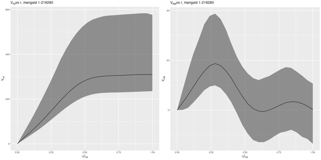
The rotational velocity is broadly similar to the polynomial model, but it has a very long plateau (the earlier model was beginning to turn over by 1 reff) and much larger uncertainty intervals. The expansion velocity curve displays completely different behavior from the polynomial model (note that the vertical scales of these two graphs are different). The mean predicted value is under 20 km/sec everywhere, and 0 is excluded only out to a radius around 6.5″, which is roughly the half length of the bar.
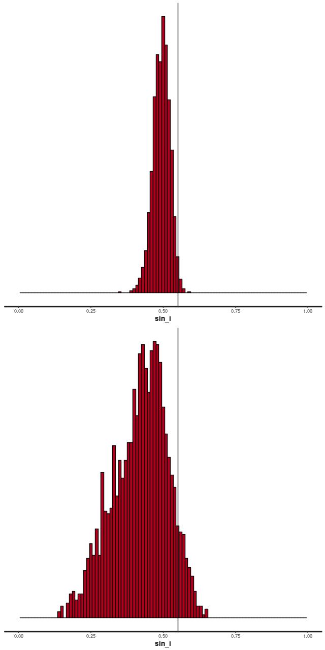
The reason for the broad credible intervals for the rotation velocity in the GP model compared to the polynomial model can be seen by comparing the posteriors of the sine of the inclination angle. The GP model’s is much broader and has a long tail towards very low inclinations. This results in a long tail of very high deprojected rotational velocities. Both models favor lower inclinations than the photometric estimate shown as a vertical line.
I’m going to leave off with one more graph. I was curious if it was really necessary to have a model for the rotation velocity, so I implemented the common pedagogical case of assuming the prior mean function is 0 (actually a constant to allow for an overall system velocity). Here are the resulting posterior predictive estimates of the rotation and expansion velocities:
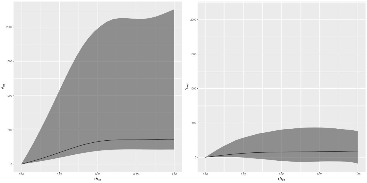
Conclusion: it is. There are several other indications of massive model failure, but these are sufficient I think.
In a future post (maybe not the next one) I’ll discuss an application that could actually produce publishable research.