One more post making use of the measurement error model introduced last time and then I think I move on. I estimate the dust attenuation of the starlight in my SFH models using a Calzetti attenuation relation parametrized by the optical depth at V (τV). If good estimates of Hα and Hβ emission line fluxes are obtained we can also make optical depth estimates of emission line regions. Just to quickly review the math we have:
\(A_\lambda = \mathrm{e}^{-\tau_V k(\lambda)}\)
where \(k(\lambda)\) is the attenuation curve normalized to 1 at V (5500Å) and \(A_\lambda\) is the fractional flux attenuation at wavelength λ. Assuming an intrinsic Balmer decrement of 2.86, which is more or less the canonical value for H II regions, the estimated optical depth at V from the observed fluxes is:
The SFH models return samples from the posteriors of the emission lines, from which are calculated sample values of \(\tau_V^{bd}\).
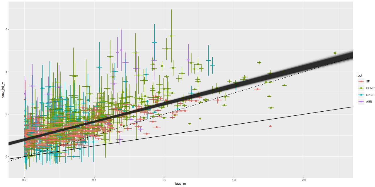
Here is a plot of the estimated attenuation from the Balmer decrement vs. the SFH model estimates for all spectra from the 28 galaxy sample in the last two posts that have BPT classifications other than no or weak emission. Error bars are ±1 standard deviation.
τVbd vs. τVstellar for 962 binned spectra in 28 MaNGA galaxies. Cloud of lines is from fit described in text. Solid and dashed lines are 1:1 and 2:1 relations.
It’s well known that attenuation in emission line regions is larger than that of the surrounding starlight, with a typical reddening ratio of ∼2 (among many references see the review by Calzetti (2001) and Charlot and Fall (2000)). One thing that’s clear in this plot that I haven’t seen explicitly mentioned in the literature is that even in the limit of no attenuation of starlight there typically is some in the emission lines. I ran the regression with measurement error model on this data set, and got the estimated relationship \(\tau_V^{bd} = 0.8 (\pm 0.05) + 1.7 ( \pm 0.09) \tau_V^{stellar}\) with a rather large estimated scatter of ≈ 0.45. So the slope is a little shallower than what’s typically assumed. The non-zero intercept seems to be a robust result, although it’s possible the models are systematically underestimating Hβ emission. I have no other reason to suspect that, though.
The large scatter shouldn’t be too much of a surprise. The shape of the attenuation curve is known to vary between and even within galaxies. Adopting a single canonical value for the Balmer decrement may be an oversimplification too, especially for regions ionized by mechanisms other than hot young stars. My models may be overdue for a more flexible prescription for attenuation.
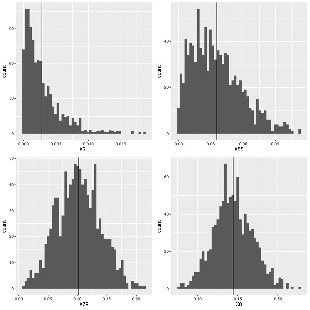
The statistical assumptions of the measurement error model are a little suspect in this data set as well. The attenuation parameter tauv is constrained to be positive in the models. When it wants to be near 0 the samples from the posterior will pile up near 0 with a tail of larger values, looking more like draws from an exponential or gamma distribution than a gaussian. Here is an example from one galaxy in the sample that happens to have a wide range of mean attenuation estimates:
Histograms of samples from the marginal posterior distributions of the parameter tauv for 4 spectra from plateifu 8080-3702.
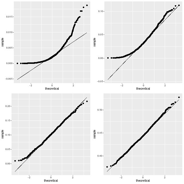
I like theoretical quantile-quantile plots better than histograms for this type of visualization:
Normal quantile-quantile plots of samples from the marginal posterior distributions of the parameter tauv for 4 spectra from plateifu 8080-3702.
I haven’t looked at the distributions of emission line ratios in much detail. They might behave strangely in some cases too. But regardless of the validity of the statistical model applied to this data set it’s apparent that there is a fairly strong correlation, which is encouraging.
Here’s a pretty common situation with astronomical data: two or more quantities are measured with nominally known uncertainties that in general will differ between observations. We’d like to explore the relationship among them, if any. After graphing the data and establishing that there is a relationship a first cut quantitative analysis would usually be a linear regression model fit to the data. But the ordinary least squares fit is biased and might be severely misleading if the measurement errors are large enough. I’m going to present a simple measurement error model formulation that’s amenable to Bayesian analysis and that I’ve implemented in Stan. This model is not my invention by the way — in the astronomical literature it dates at least to Kelly (2007), who also explored a number of generalizations. I’m only going to discuss the simplest case of a single predictor or covariate, and I’m also going to assume all conditional distributions are gaussian.
The basic idea of the model is that the real, unknown quantities (statisticians call these latent variables, and so will I) are related through a linear regression. The conditional distribution of the latent dependent variable is
where \(\sigma_{x, i}, \sigma_{y, i}\) are the known standard deviations. The full joint distribution is completed by specifying priors for the parameters \(\beta_0, \beta_1, \sigma\). This model is very easy to implement in the Stan language and the complete code is listed below. I’ve also uploaded the code, a script to reproduce the simulated data example discussed below, and the SFR-stellar mass data from the last page in a dropbox folder.
Most of this code should be self explanatory, but there are a few things to note. In the transformed data section I standardize both variables, that is I subtract the means and divide by the standard deviations. The individual observation standard deviations are also scaled. The transformed parameters block is strictly optional in this model. All it does is spell out the linear part of the linear regression model.
In the model block I give a very vague prior for the latent x variables. This has almost no effect on the model output since the posterior distributions of the latent values are strongly constrained by the observed data. The parameters of the regression model are given less vague priors. Since we standardized the data we know beta0 should be centered near 0 and beta1 near 1 and all three should be approximately unit scaled. The rest of the model block just encodes the conditional distributions I wrote out above.
Finally the generated quantities block does two things: generate some some new simulated data values under the model using the sampled parameters, and rescale the parameter values to the original data scale. The first task enables what’s called “posterior predictive checking.” Informally the idea is that if the model is successful simulated data generated under it should look like the data that was input.
It’s always a good idea to try out a model with some simulated data that conforms to it, so here’s a script to generate some data, then print and graph some basic results. This is also in the dropbox folder.
Inference for Stan model: ls_me.
4 chains, each with iter=2000; warmup=1000; thin=1;
post-warmup draws per chain=1000, total post-warmup draws=4000.

             mean se_mean    sd  2.5%   25%   50%    75%  97.5% n_eff  Rhat
b0          9.995   0.001 0.042 9.912 9.966 9.994 10.023 10.078  5041 0.999
b1          1.993   0.001 0.040 1.916 1.965 1.993  2.020  2.073  4478 1.000
sigma_unorm 0.472   0.001 0.037 0.402 0.447 0.471  0.496  0.549  2459 1.003

Samples were drawn using NUTS(diag_e) at Thu Jan  9 10:09:34 2020.
For each parameter, n_eff is a crude measure of effective sample size,
and Rhat is the potential scale reduction factor on split chains (at
convergence, Rhat=1).
>
and graph:
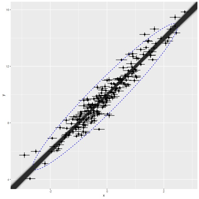
Simulated data and model fit from script in text. Ellipse is 95% confidence interval for new data generated from model.
This all looks pretty good. The true parameters are well within the 95% confidence bounds of the estimates. In the graph the simulated new data is summarized with a 95% confidence ellipse, which encloses just about 95% of the input data, so the posterior predictive check indicates a good model. Stan is quite aggressive at flagging potential convergence failures, and no warnings were generated.
Turning to some real data I also included in the dropbox folder the star formation rate density versus stellar mass density data that I discussed in the last post. This is in something called R “dump” format, which is just an ascii file with R assignment statements for the input data. This isn’t actually a convenient form for input to rstan’s sampler or ggplot2’s plotting commands, so once loaded the data are copied into a list and a data frame. The interactive session for analyzing the data was:
Star formation rate vs. Stellar mass for star forming regions. Data from previous post.
Semi-transparent lines – model fits to the regression line as described in text.
Dashed red line – “orthogonal distance regression” fit.
Inference for Stan model: ls_me.
4 chains, each with iter=2000; warmup=1000; thin=1;
post-warmup draws per chain=1000, total post-warmup draws=4000.

              mean se_mean   sd   2.5%    25%    50%    75%  97.5% n_eff Rhat
b0          -11.20       0 0.26 -11.73 -11.37 -11.19 -11.02 -10.67  7429    1
b1            1.18       0 0.03   1.12   1.16   1.18   1.20   1.24  7453    1
sigma_unorm   0.27       0 0.01   0.25   0.27   0.27   0.28   0.29  7385    1

Samples were drawn using NUTS(diag_e) at Thu Jan  9 10:49:42 2020.
For each parameter, n_eff is a crude measure of effective sample size,
and Rhat is the potential scale reduction factor on split chains (at
convergence, Rhat=1).
Once again the model seems to fit the data pretty well, the posterior predictive check is reasonable, and Stan didn’t complain. Astronomers are often interested in the “cosmic variance” of various quantities, that is the true amount of unaccounted for variation. If the error estimates in this data set are reasonable the cosmic variance in SFR density is estimated by the parameter σ. The mean estimate of around 0.3 dex is consistent with other estimates in the literature1see the compilation in the paper by Speagle et al. that I cited last time, for example.
I noticed in preparing the last post that several authors have used something called “orthogonal distance regression” (ODR) to estimate the star forming main sequence relationship. I don’t know much about the technique besides that it’s an errors in variables regression method. There is an R implementation in the package pracma. The red dashed line in the plot above is the estimate for this dataset. The estimated slope (1.41) is much steeper than the range of estimates from this model. On casual visual inspection though it’s not clearly worse at capturing the mean relationship.
It took a few months but I did manage to analyze 28 of the 29 galaxies in the sample I introduced last time. One member — mangaid 1-604907 — hosts a broad line AGN and has broad emission lines throughout. That’s not favorable for my modeling methods, so I left it out. It took a while to develop a more or less standardized analysis protocol, so there may be some variation in S/N cuts in binning the spectra and in details of model runs in Stan. Most runs used 250 warmup and 750 total iterations for each of 4 chains run in parallel, with some adaptation parameters changed from their default values1I set target acceptance probability adapt_delta to 0.925 or 0.95 and the maximum treedepth for the No U-Turn Sampler max_treedepth to 11-12. A total post-warmup sample size of 2000 is enough for the inferences I want to make. One of the major advantages of the NUTS sampler is that once it converges it tends to produce draws from the posterior with very low autocorrelation, so effective sample sizes tend to be close to the number of samples.
I’m just going to look at a few measured properties of the sample in this post. In future ones I may look in more detail at some individual galaxies or the sample as a whole. Without a control sample it’s hard to say if this one is significantly different from a randomly chosen sample of galaxies, and I’m not going to try. In the plots shown below each point represents measurements on a single binned spectrum. The number of binned spectra per galaxy ranged from 15 to 153 with a median of 51.5, so a relatively small number of galaxies contribute disproportionately to these plots.
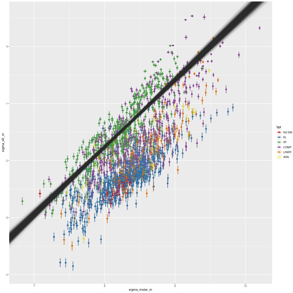
One of the more important empirical results in extragalactic astrophysics is the existence of a fairly well defined and approximately linear relationship between stellar mass and star formation rate for star forming galaxies, which has come to be known as the “star forming main sequence.” Thanks to CALIFA and MaNGA it’s been established in recent years that the SFMS extends to subgalactic scales as well, at least down to the ∼kpc resolution of these surveys. This first plot is of the star formation rate surface density vs. stellar mass surface density, where recall my estimate of SFR is for a time scale of 100 Myr. Units are \(\mathrm{M_\odot /yr/kpc^2} \) and \(\mathrm{M_\odot /kpc^2} \), logarithmically scaled. These estimates are uncorrected for inclination and are color coded by BPT class using Kauffmann’s classification scheme for [N II] 6584, with two additional classes for spectra with weak or no emission lines.
If we take spectra with star forming line ratios as comprising the SFMS there is a fairly tight relation: the cloud of lines are estimates from a Bayesian simple linear regression with measurement error model fit to the points with star forming BPT classification only (N = 428). The modeled relationship is \(\Sigma_{sfr} = -11.2 (\pm 0.5) + 1.18 (\pm 0.06)~ \Sigma_{M^*}\) (95% marginal confidence limits), with a scatter around the mean relation of ≈ 0.27 dex. The slope here is rather steeper than most estimates2For example in a large compilation by Speagle et al. (2014) none of the estimates exceeded a slope of 1., but perhaps coincidentally is very close to an estimate for a small sample of MaNGA starforming galaxies in Lin et al. (2019). I don’t assign any particular significance to this result. The slope of the SFMS is highly sensitive to the fitting method used, the SFR and stellar mass calibrators, and selection effects. Also, the slope and intercept estimates are highly correlated for both Bayesian and frequentist fitting methods.
One notable feature of this plot is the rather clear stratification by BPT class, with regions having AGN/LINER line ratios and weak emission line regions offset downwards by ~1 dex. Interestingly, regions with “composite” line ratios straddle both sides of the main sequence, with some of the largest outliers on the high side. This is mostly due to the presence of Markarian 848 in the sample, which we saw in recent posts has composite line ratios in most of the area of the IFU footprint and high star formation rates near the northern nucleus (with even more hidden by dust).
Σsfr vs. ΣM*. Cloud of straight lines is an estimate of the star-forming main sequence relation based on spectra with star-forming line ratios. Sample is all analyzed spectra from the set of “transitional” candidates of the previous post.
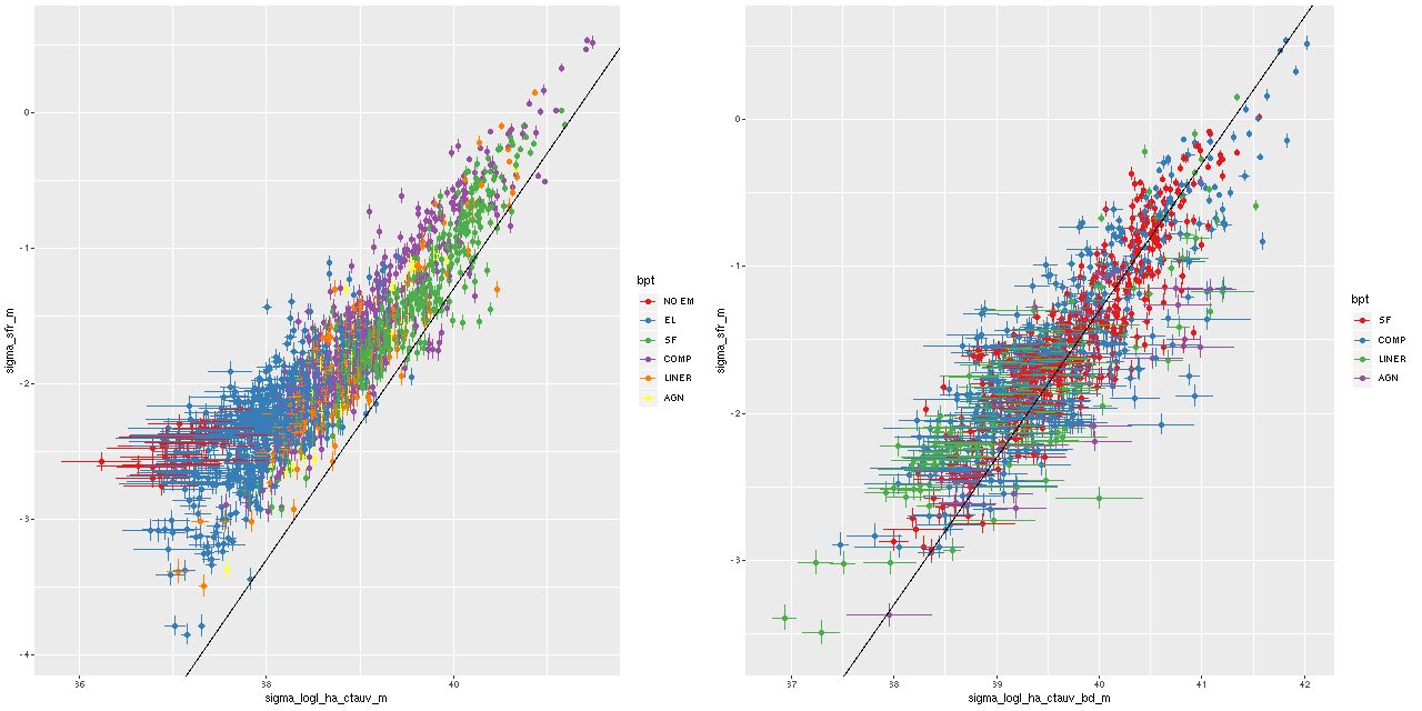
Another notable relationship that I’ve shown previously for a few individual galaxies is between the star formation rate estimated from the SFH models and Hα luminosity, which is the main SFR calibrator in optical spectra. In the left hand plot below Hα is corrected for the estimated attenuation for the stellar component in the SFH models. The straight line is the SFR-Hα calibration of Moustakas et al. (2006), which can be traced back to early ’90s work by Kennicutt.
Most of the sample does follow a linear relationship between SFR density and Hα luminosity density with an offset from the Kennicutt-Moustakas calibration, but there appears to be a departure from linearity at the low SFR end in the sense that the 100 Myr averaged SFR exceeds the amount predicted by Hα (which recall traces star formation on 5-10 Myr scales). This might be interpreted as indicating that the sample includes a significant number of regions that have been very recently quenched (that is within the past 10-100 Myr). There are other possible interpretation though, including biased estimates of Hα luminosity when emission lines are weak.
In the right hand panel below I plot the same relationship but with Hα corrected for attenuation using the Balmer decrement for spectra with firm detections in the four lines that go into the [N II]/Hα vs. [O III]/Hβ BPT classification, and therefore have firm detections in Hβ. The sample now nicely straddles the calibration line over the ∼ 4 orders of magnitude of SFR density estimates. So, the attenuation in the regions where emission lines arise is systematically higher than the estimated attenuation of stellar light. This is a well known result. What’s encouraging is it implies my model attenuation estimates actually contain useful information.
(L) Estimated Σsfr vs. Σlog L(Hα) corrected for attenuation using stellar attenuation estimate.
(R) same but Hα luminosity corrected using Balmer decrement. Spectra with detected Hβ emission only.
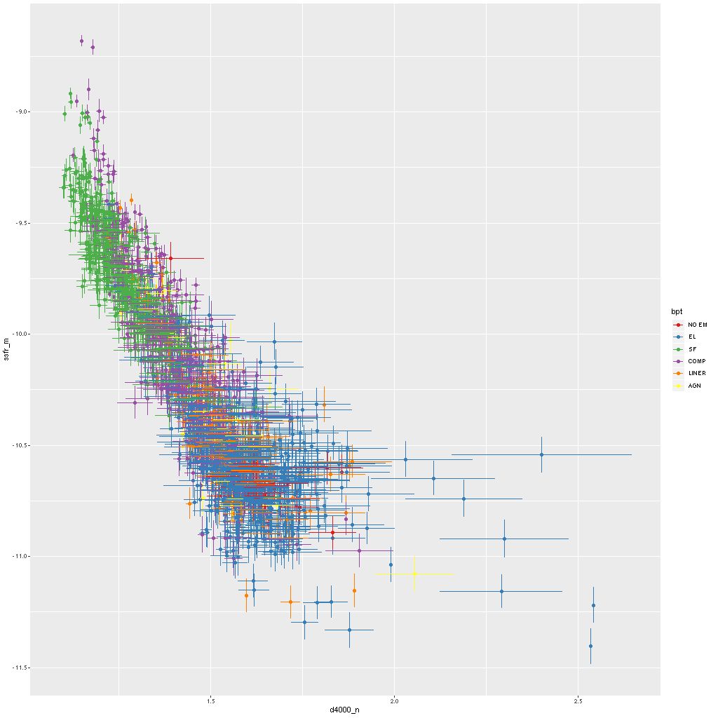
One final relation: some measure of the 4000Å break strength has been used as a calibrator of specific star formation rate since at least Brinchmann et al. (2004). Below is my version using the “narrow” definition of D4000. I haven’t attempted a quantitative comparison with any other work, but clearly there’s a well defined relationship. Maybe worth noting is that “red and dead” ETGs typically have \(\mathrm{D_n(4000)} \gtrsim 1.75\) (see my previous post for example). Very few of the spectra in this sample fall in that region, and most are low S/N spectra in the outskirts of a few of the galaxies.
Specific star formation rate vs. Dn4000
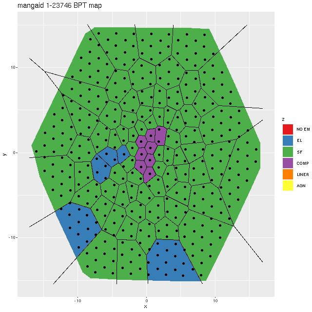
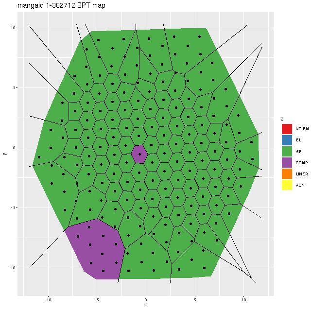
Two obvious false positives in this sample were a pair of grand design spirals (mangaids 1-23746 and 1.382712) with H II regions sprinkled along the full length of their arms. To see why they were selected and verify that they’re in fact false positives here are BPT maps:
Map of BPT classification — mangaid 1-23746 (plateifu 8611-12702)Map of BPT classification — mangaid 1-382712 (plateifu 9491-6101)
These are perfect illustrations of the perils of using single fiber spectra for sample selection when global galaxy properties are of interest. The central regions of both galaxies have “composite” spectra, which might actually indicate that the emission is from a combination of AGN and star forming regions, but outside the nuclear regions star forming line ratios prevail throughout.
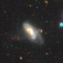
These two galaxies contribute about 45% of the binned spectra with star forming line ratios, so the SFMS would be much more sparsely populated without their contribution. Only one other galaxy (mangaid 1-523050) is similarly dominated by SF regions and it has significantly disturbed morphology.
I may return to this sample or individual members in the future. Probably my next posts will be about Bayesian modelling though.
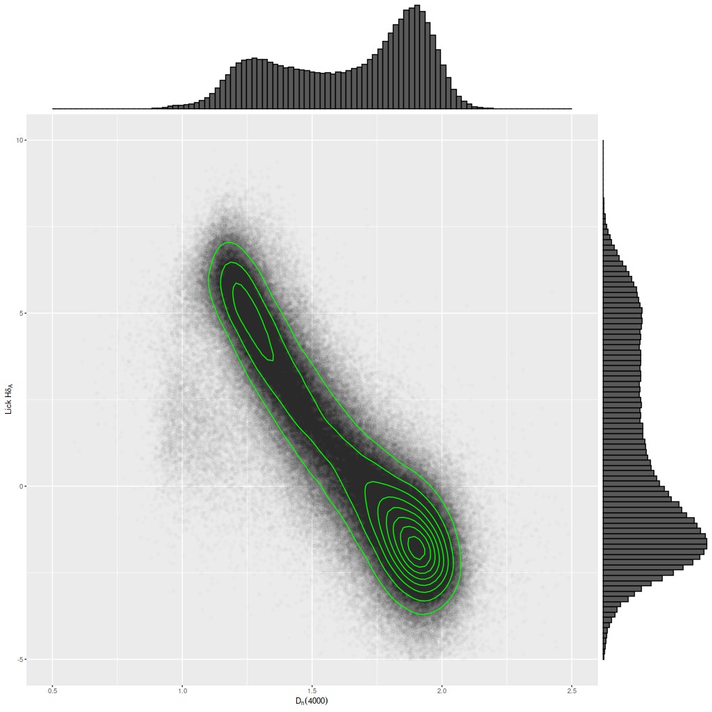
I’ve mentioned a few times that I took a shot several years ago at selecting a sample of post-starburst, or to use a term that’s gained some currency recently, “transitioning” galaxies1transitioning in this context implies that star formation has recently ceased or is in the process of shutting down. To cite one example Alatalo et al. (2017) use the word 18 times with this meaning. One thing that astronomers have come to realize is that traditional K+A spectroscopic selection criteria (basically requiring a combination of strong Balmer absorption lines and weak emission) potentially miss important populations, for example galaxies hosting an AGN. Selecting for weak emission also implies that star formation has already shut down, which precludes finding galaxies that are in the process of shutting down but still forming stars. On the other hand simply dropping constraints on emission won’t work because the resulting sample would be contaminated with a large fraction of normal star forming galaxies. Here is a popular spectroscopic diagnostic diagram, plotting the (pseudo) Lick HδA index against the 4000Å break strength index Dn(4000). This version used the MPA-JHU measurements for approximately 1/2 of SDSS single fiber galaxy spectra from DR8.
The lick Hδ – 4000Å break strength plane for a large sample of SDSS galaxies. Measurements from the MPA-JHU pipeline.
As is true of many observed properties of galaxies the distribution in this diagram is strongly bimodal, with one of the modes centered right around HδA ≈ 5Å. For the most part this region of the Hδ-D4000 plane is occupied by starforming galaxies — somewhere around 8-10% of all SDSS spectra with MPA measurements have HδA ≥ 5Å, while true K+A galaxies are no more than a fraction of a percent of the local population. I took the simplest possible approach to try to minimize contamination from starforming galaxies: besides a traditional K+A selection with slightly relaxed emission line constraints I made a selection of spectra with emission line ratios in the “other than starforming” region of the [N II]/Hα vs [O III]/Hβ BPT diagnostic. I decided to use Kauffmann’s empirical starforming boundary as the selection criterion, and therefore included the so-called “composite” region of the BPT diagnostic. For the sake of completeness and reproducibility here is part of the CASJobs query I used. I saved a number of measurements from the MPA spectroscopic pipeline as well as the SDSS photo pipeline that aren’t included in the listing below. I did include a few lines just to point out that it’s important to use the emission line subtracted version of the Lick Hδ index because it can be significantly contaminated. Most of the where clause of the query is selecting spectra with firm detections and good error estimates of the relevant emission and absorption lines. There is also a redshift range constraint — the upper limit is set to avoid contamination of Hδ by the 5577Å terrestrial night sky line. Finally there are some modest quality constraints.
select into mydb.kaufpostagn
  gi.lick_hd_a_sub as lick_hd_a,
  gi.lick_hd_a_sub_err as lick_hd_a_err,
  gi.d4000_n,
  gi.d4000_n_err
from specObj s
  left outer join PhotoObj as p on s.bestObjid = p.Objid
  left outer join galSpecline as g on s.specObjid = g.specObjid
  left outer join galSpecIndx as gi on s.specObjid = gi.specObjid
  left outer join galSpecExtra as ge on s.specObjid = ge.specObjid
  where
  (g.h_alpha_flux/g.h_alpha_flux_err > 3 and g.h_alpha_flux_err > 0) and
  (g.nii_6584_flux/g.nii_6584_flux_err > 3 and g.nii_6584_flux_err > 0) and
  (g.h_beta_flux/g.h_beta_flux_err > 3 and g.h_beta_flux_err > 0) and
  (g.oiii_flux/g.oiii_flux_err > 3 and g.oiii_flux_err > 0) and
  ((0.61/(log10(g.nii_6584_flux/g.h_alpha_flux)-0.05)+1.3 <
    log10(g.oiii_flux/g.h_beta_flux)) or (log10(g.nii_6584_flux/g.h_alpha_flux)>=0.05)) and
  (gi.lick_hd_a_sub > 5 and gi.lick_hd_a_sub_err > 0) and
  (s.z > .02 and s.z < 0.35) and
  (s.snMedian > 10) and
  (s.zWarning = 0 or s.zWarning = 16)
  order by
  s.plate, s.mjd, s.fiberid
I used a second query to make a more traditional K+A selection. This all could have been done with a single query but the conditions get a bit complicated. These queries run in the DR10 “context”2the data release doesn’t actually matter as long as it’s later than DR7 since the last release the MPA pipeline was run on was DR8. should return 4,235 and 874 hits respectively, with some overlap.
select into mydb.myka
s.ra,
s.dec,
s.plate,
s.mjd,
s.fiberid,
s.specObjid,
from specObj s
left outer join PhotoObj as p on s.bestObjid = p.Objid
left outer join galSpecline as g on s.specObjid = g.specObjid
left outer join galSpecIndx as gi on s.specObjid = gi.specObjid
left outer join galSpecExtra as ge on s.specObjid = ge.specObjid
where
  (g.oii_3729_eqw > -5 and g.oii_3729_eqw_err > 0) and
  (g.h_alpha_eqw >  -5 and g.h_alpha_eqw_err > 0) and
  (gi.lick_hd_a_sub > 5 and gi.lick_hd_a_sub_err > 0) and
  (s.z > .02 and s.z < 0.35) and
  (s.snMedian > 10) and
  (s.zWarning = 0 or s.zWarning = 16)
order by
  s.plate, s.mjd, s.fiberid
I thought at the time based solely on examining SDSS thumbnails that there were rather too many false positives in the form of normal starforming galaxies for the intended purpose of the sample. The choice to include galaxies in Kauffmann’s composite region played some role in this — although even the people responsible for this classification scheme admit now that it’s too simple some galaxies really do have spectra that are composites of starforming regions and AGN. But the more important reason I think is the well known problem that single fiber spectra only cover a portion of most nearby galaxies and galaxy nuclei (which were the intended targets) just aren’t representative of the global properties of galaxies. The SPOGS3an acronym formed somehow from the term “shocked post-starburst galaxy survey.” sample of Alatalo et al. 2016, which has similar aims to my selection but more elaborate selection criteria, has (in my opinion) a similar issue of false positives for the same reason.
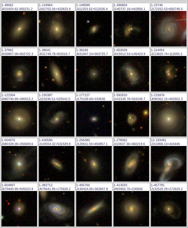
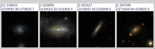
MaNGA provides a unique opportunity to examine the causes of false positives in my transitional sample, and I hope also confirm some real positives. A simple position crossmatch of my sample, which has about 5500 members, with MaNGA DR15 object coordinates produced 29 matches with a position tolerance of about 3″. SDSS thumbnails of the 29 are shown below. By my count at least 13, or 45%, of the sample are visibly disturbed in some way with 7 of those being clear merger remnants with evident shells and tidal tails.
I’ve been calculating star formation history models for these at a leisurely pace and plan to write more about the sample in future posts. Two of these I’ve already written about — besides Mrk 848 number 15 in the postage stamps was the subject of a series of posts starting here. I may write more case studies like those, or perhaps take a more holistic look at the sample and compare to a control group.
As something of an aside, with a looser position matching tolerance a 30th object turns up:
CGCG 390-0666 (SDSS finder chart image)
CGCG 390-066 (Legacy survey cutout)
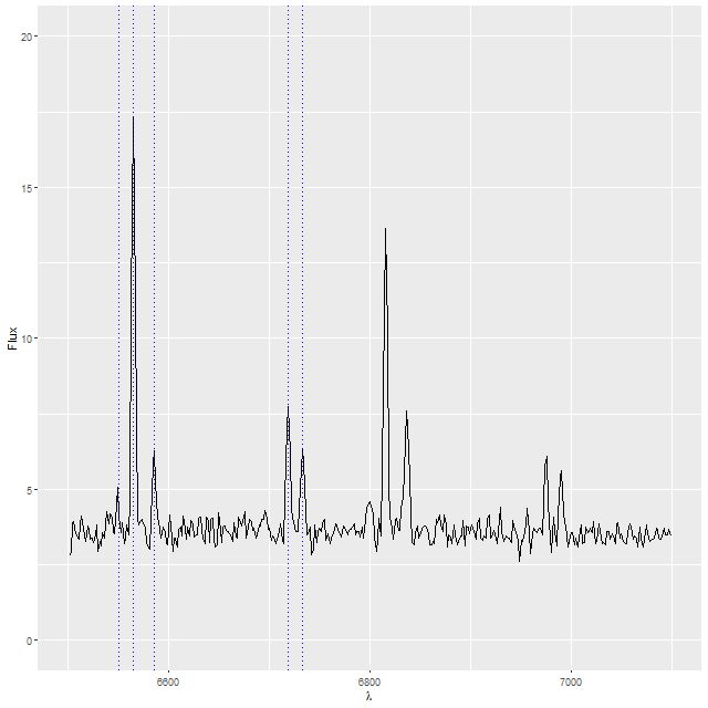
This made my sample based on the spectrum of the eastern nucleus. This object turns out to be doubly strange. Besides having two apparent nuclei, when I did some preliminary spectral fitting I noticed a peculiar pattern of residuals that turned out to be due to this:
Extract from a single spectrum of plateifu 8083-9101 (mangaid 1-38017)
Many of the spectra have emission lines at exactly their rest frame wavelengths. This particular spectrum, which came from somewhere in the SE quadrant of the IFU footprint, clearly shows Hα plus the [N II] and [S II] doublets offset from the same lines at the redshift of the galaxy. It turns out this galaxy lies near the edge of the Orion-Eridanus superbubble, a large region of diffuse emission in our galaxy. Should I choose to study this galaxy in more detail these lines could be masked easily enough, but the metadata for this data cube says it shouldn’t be used.
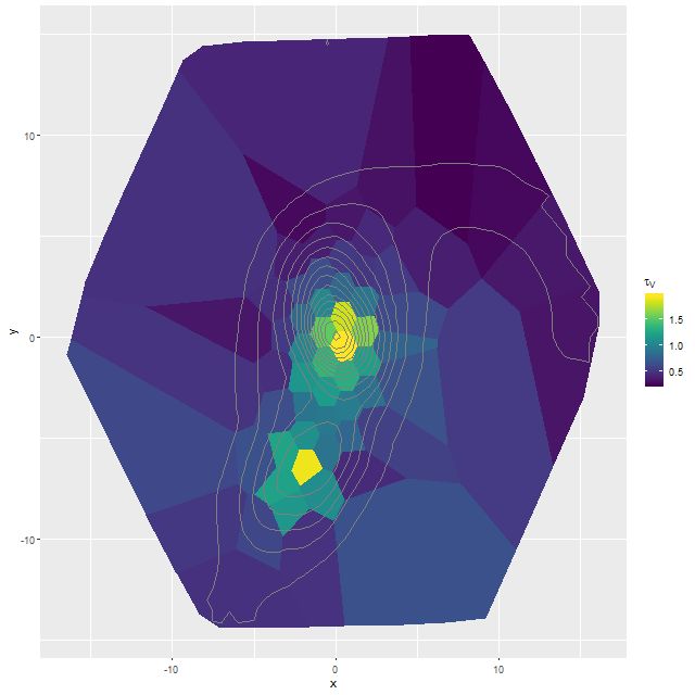
I’m going to close out my analysis of Mrk 848 for now with three topics. First, dust. Like most SED fitting codes mine produces an estimate of the internal attenuation, which I parameterize with τV, the optical depth at V assuming a conventional Calzetti attenuation curve. Before getting into a discussion for context here is a map of the posterior mean estimate for the higher S/N target binning of the data. For reference isophotes of the synthesized r band surface brightness taken from the MaNGA data cube are superimposed:
Map of posterior mean of τV from single component dust model fits with Calzetti attenuation
This compares reasonably well with my visual impression of the dust distribution. Both nuclei have very large dust optical depths with a gradual decline outside, while the northern tidal tail has relatively little attenuation.
The paper by Yuan et al. that I looked at last time devoted most of its space to different ways of modeling dust attenuation, ultimately concluding that a two component dust model of the sort advocated by Charlot and Fall (2000) was needed to bring results of full spectral fitting using ppxf on the same MaNGA data as I’ve examined into reasonable agreement with broad band UV-IR SED fits.
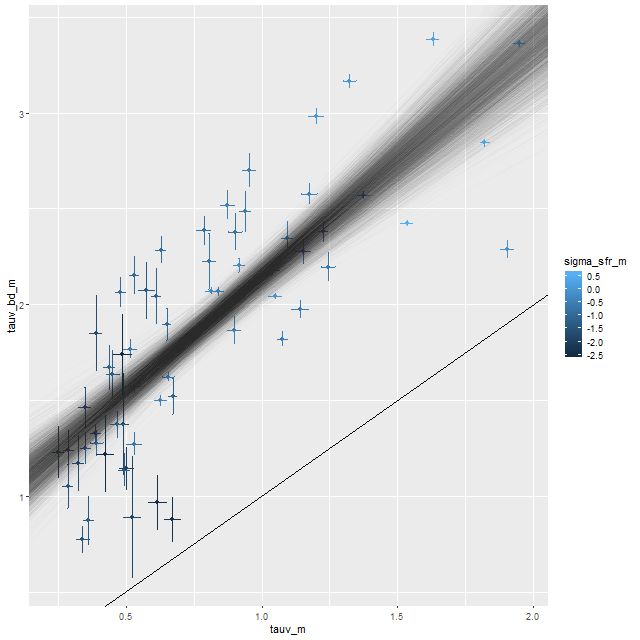
There’s certainly some evidence in support of this. Here is a plot I’ve shown for some other systems of the estimated optical depth of the Balmer emission line emitting regions based on the observed vs. theoretical Balmer decrement (I’ve assumed an intrinsic Hα/Hβ ratio of 2.86 and a Calzetti attenuation relation) plotted against the optical depth estimated from the SFH models, which roughly estimates the amount of reddening needed to fit the SSP model spectra to the observed continuum. In some respects this is a more favorable system than some I’ve looked at because Hβ emission is at measurable levels throughout. On the other hand there is clear evidence that multiple ionization mechanisms are at work, so the assumption of a single canonical value of Hα/Hβ is likely too simple. This might be a partial cause of the scatter in the modeled relationship, but it’s encouraging that there is a strong positive correlation (for those who care, the correlation coefficient between the mean values is 0.8).
The solid line in the graph below is 1:1. The semi-transparent cloud of lines are the sampled relationships from a Bayesian errors in variables regression model. The mean (and marginal 1σ uncertainty) is \(\tau_{V, bd} = (0.94\pm 0.11) + (1.21 \pm 0.12) \tau_V\). So the estimated relationship is just a little steeper than 1:1 but with an offset of about 1, which is a little different from the Charlot & Fall model and from what Yuan et al. found, where the youngest stellar component has about 2-3 times the dust attenuation as the older stellar population. I’ve seen a similar not so steep relationship in every system I’ve looked at and don’t know why it differs from what is typically assumed. I may look into it some day.
τV estimated from Balmer decrement vs. τV from model fits. Straight line is 1:1 relation. Cloud of lines are from Bayesian errors in variables regression model.
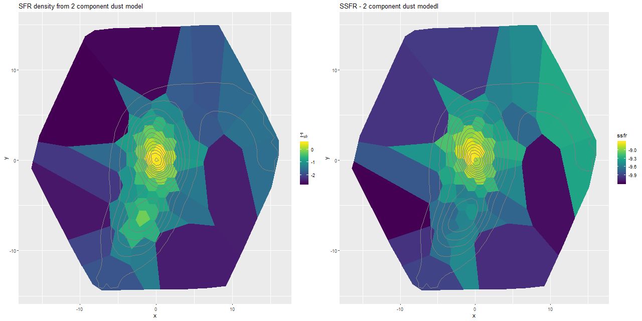
I did have time to run some 2 dust component SFH models. This is a very simple extension of the single component models: a single optical depth is applied to all SSP spectra. A second component with the optical depth fixed at 1 larger than the bulk value is applied only to the youngest model spectra, which recall were taken from unevolved SSPs from the updated BC03 library. I’m just going to show the most basic results from the models for now in the form of maps of the SFR density and specific star formation rate. Compared to the same maps displayed at the end of the last post there is very little difference in spatial variation of these quantities. The main effect of adding more reddened young populations to the model is to replace some of the older light — this is the well known dust-age degeneracy. The average effect was to increase the stellar mass density (by ≈ 0.05 dex overall) while slightly decreasing the 100Myr average SFR (by ≈ 0.04 dex), leading to an average decrease in specific star formation rate of ≈ 0.09 dex. While there are some spatial variations in all of these quantities no qualitative conclusion changes very much.
Results from fits with 2 component dust models.
(L) SFR density.
(R) Specific SFR
Contrary to Yuan+ I don’t find a clear need for a 2 component dust model. Without trying to replicate their results I can’t say why exactly we disagree, but I think they erred in aggregating the MaNGA data to the lowest spatial resolution of the broad band photometric data they used, which was 5″ radius. There are clear variations in physical conditions on much smaller scales than this.
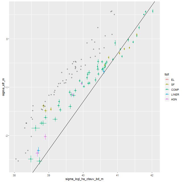
Second topic: the most widely accepted SFR indicator in visual wavelengths is Hα luminosity. Here is another plot I’ve displayed previously: a simple scatterplot of Hα luminosity density against the 100Myr averaged star formation rate density from the SFH models. Luminosity density is corrected for attenuation estimated from the Balmer decrement and for comparison the light gray points are the uncorrected values. Points are color coded by BPT class determined in the usual manner. The straight line is the Hα – SFR calibration of Moustakas et al. (2006), which in turn is taken from earlier work by Kennicutt.
Model SFR density vs. Hα luminosity density corrected for extinction estimated from Balmer decrement. Light colored points are uncorrected for extinction. Straight line is Hα-SFR calibration from Moustakas et al. (2006)
Keeping in mind that Hα emission tracks star formation on timescales of ∼10 Myr1to the extent that ionization is caused by hot young stars. There are evidently multiple ionizing sources in this system, but disentangling their effects seems hard. Note there’s no clear stratification by BPT class in this plot. this graph strongly supports the scenario I outlined in the last post. At the highest Hα luminosities the SFR-Hα trend nicely straddles the Kennicutt-Moustakas calibration, consistent with the finding that the central regions of the two galaxies have had ∼constant or slowly rising star formation rates in the recent past. At lower Hα luminosities the 100Myr average trends consistently above the calibration line, implying a recent fading of star formation.
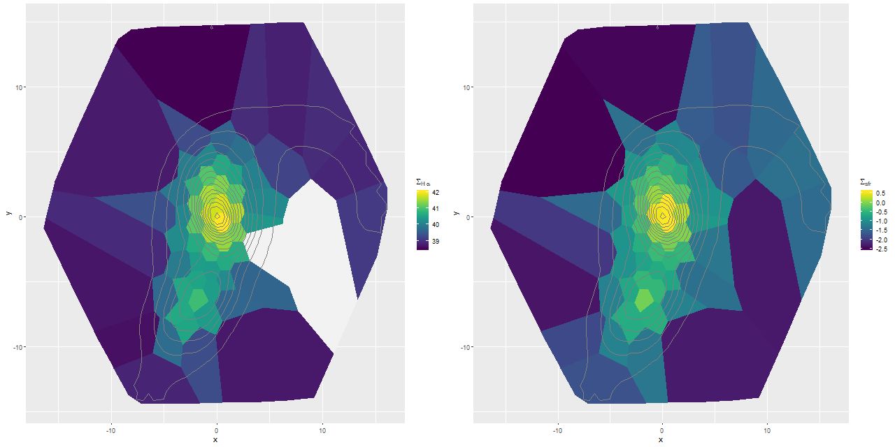
The maps below add some detail, and here the perceptual uniformity of the viridis color palette really helps. If star formation exactly tracked Hα luminosity these two maps would look the same. Instead the northern tidal tail in particular and the small piece of the southern one within the IFU footprint are underluminous in Hα, again implying a recent fading of star formation in the peripheries.
(L) Hα luminosity density, corrected for extinction estimated by Balmer decrement.
(R) SFR density (100 Myr average).
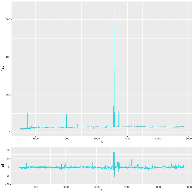
Final topic: the fit to the data, and in particular the emission lines. As I’ve mentioned previously I fit the stellar contribution and emission lines simultaneously, generally assuming separate single component gaussian velocity dispersions and a common system velocity offset. This works well for most galaxies, but for active galaxies or systems like this one with complex velocity profiles maybe not so much. In particular the northern nuclear region is known to have high velocity outflows in both ionized and neutral gas due presumably to supernova driven winds. I’m just going to look at the central fiber spectrum for now. I haven’t examined the fits in detail, but in general they get better outside the immediate region of the center. First, here is the fit to the data using my standard model. In the top panel the gray line, which mostly can’t be seen, is the observed spectrum. Blue are quantiles of the posterior mean fit — this is actually a ribbon, although its width is too thin to be discernable. The bottom panel are the residuals in standard deviations. Yes, they run as large as ±50σ, with conspicuous problems around all emission lines. There are also a number of usually weak emission lines that I don’t track that are present in this spectrum.
Fit to central fiber spectrum; model with single gaussian velocity distributions.
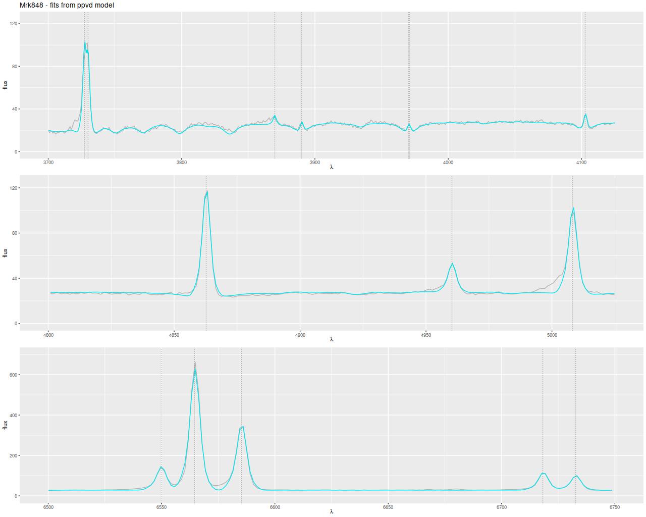
I have a solution for cases like this which I call partially parametric. I assume the usual Gauss-Hermite form for the emission lines (as in, for example, ppxf) while the stellar velocity distribution is modeled with a convolution kernel2I think I’ve discussed this previously but I’m too lazy to check right now. If I haven’t I’ll post about it someday. Unfortunately the Stan implementation of this model takes at least an order of magnitude longer to execute than my standard one, which makes its wholesale use prohibitively expensive. It does materially improve the fit to this spectrum although there are still problems with the stronger emission lines. Let’s zoom in on a few crucial regions of the spectrum:
Zoomed in fit to central fiber spectrum using “partially parametric velocity distribution” model. Grey: observed flux. Blue: model.
The two things that are evident here are the clear sign of outflow in the forbidden emission lines, particularly [O III] and [N II], while the Balmer lines are relatively more symmetrical as are the [S II] doublet at 6717, 6730Å. The existence of rather significant residuals is likely because emission is coming from at least two physically distinct regions while the fit to the data is mostly driven by Hα, which as usual is the strongest emission line. The fit captures the emission line cores in the high order Balmer lines rather well and also the absorption lines on the blue side of the 4000Å break except for the region around the [Ne III] line at 3869Å.
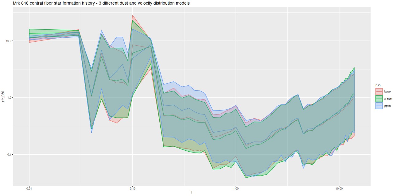
I’m mostly interested in star formation histories, and it’s important to see what differences are present. Here is a comparison of three models: my standard one, the two dust component model, and the partially parametric velocity dispersion model:
Detailed star formation history models for the northern nucleus using 3 different models.
In fact the differences are small and not clearly outside the range of normal MCMC variability. The two dust model slightly increases the contribution of the youngest stellar component at the expense of slightly older contributors. All three have the presumably artifactual uptick in SFR at 4Gyr and very similar estimated histories for ages >1 Gyr.
I still envision a number of future model refinements. The current version of the official data analysis pipeline tracks several more emission lines than I do at present and has updated wavelengths that may be more accurate than the ones from the SDSS spectro pipeline. It might be useful to allow at least two distinct emission line velocity distributions, with for example one for recombination lines and one for forbidden. Unfortunately the computational expense of this sort of generalization at present is prohibitive.
I’m not impressed with the two dust model that I tried, but there may still be useful refinements to the attenuation model to be made. A more flexible form of the Calzetti relation might be useful for example3there is recent relevant literature on this topic that I’m again too lazy to look up.
My initial impression of this system was that it was a clear false positive that was selected mostly because of a spurious BPT classification. On further reflection with MaNGA data available it’s not so clear. A slight surprise is the strong Balmer absorption virtually throughout the system with evidence for a recent shut down of star formation in the tidal tails. A popular scenario for the formation of K+A galaxies through major mergers is that they experience a centrally concentrated starburst after coalescence which, once the dust clears and assuming that some feedback mechanism shuts off star formation leads to a period of up to a Gyr or so with a classic K+A signature4I previously cited Bekki et al. 2005, who examine this scenario in considerable detail.Capturing a merger in the instant before final coalescence provides important clues about this process.
To the best of my knowledge there have been no attempts at dynamical modeling of this particular system. There is now reasonably good kinematic information for the region covered by the MaNGA IFU, and there is good photometric data from both HST and several imaging surveys. Together these make detailed dynamical modeling technically feasible. It would be interesting if star formation histories could further constrain such models. Being aware of the multiple “degeneracies” between stellar age and other physical properties I’m not highly confident, but it seems provocative that we can apparently identify distinct stages in the evolutionary history of this system.
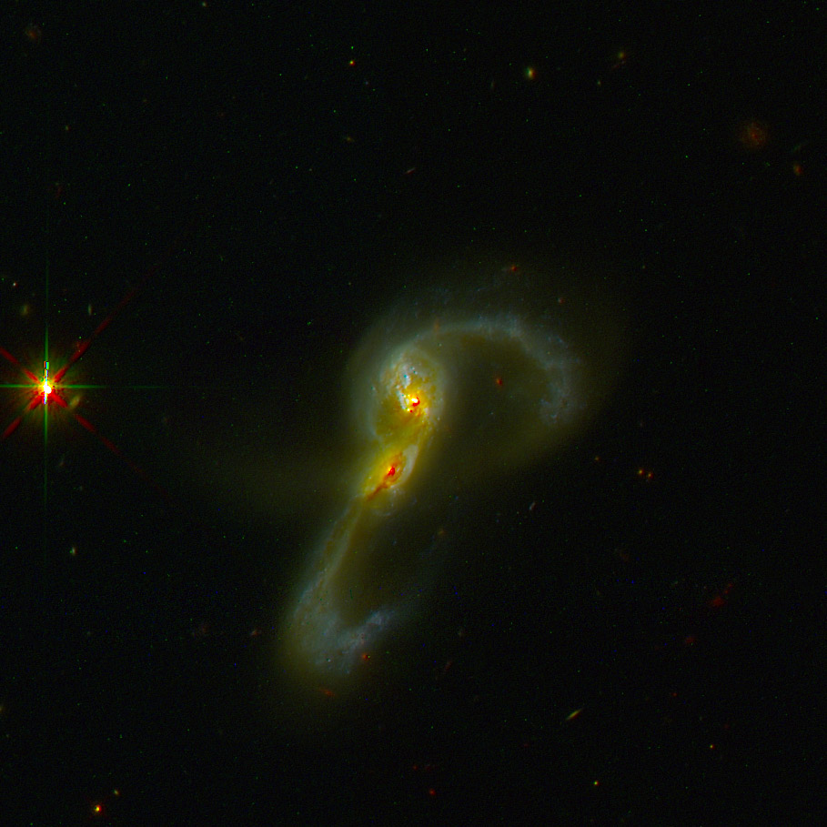
In this post I’m going to take a quick look at detailed, spatially resolved star formation histories for this galaxy pair and briefly compare to some of the recent literature. Before I start though, here is a reprocessed version of the blog’s cover picture with a different crop and some Photoshop curve and level adjustments to brighten the tidal tails a bit. Also I cleaned up some more of the cosmic ray hits.
Markarian 848 – full resolution crop with level curve adjustment
HST ACS/WFC F435W/F814W/F160 false color image
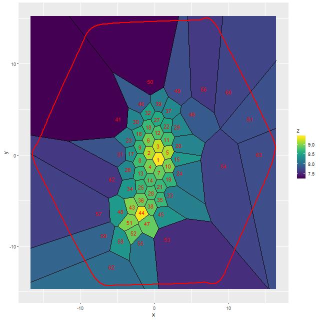
The SFH models I’m going to discuss were based on MaNGA data binned to a more conservative signal to noise target than in the last post. I set a target S/N of 25 — Cappellari’s Voronoi binning algorithm has a hard coded acceptance threshold of 80% of the target S/N, which results in all but a few bins having an actual S/N of at least 20. This produced a binned data set with 63 bins. The map below plots the modeled (posterior mean log) stellar mass density, with clear local peaks in the bins covering the positions of the two nuclei. The bins are numbered in order of increasing distance of the weighted centroids from the IFU center, which corresponds with the position of the northern nucleus. The center of bin 1 is slightly offset from the northern nucleus by about 2/3″. For reference the angular scale at the system redshift (z ≈ 0.040) is 0.8 kpc/” and the area covered by each fiber is 2 kpc2.
Although there’s nothing in the Voronoi binning algorithm that guarantees this it did a nice job of partitioning the data into physically distinct regions, with the two nuclei, the area around the northern nucleus, and the bridge between them all binned to single fiber spectra. The tidal tails are sliced into several pieces while the very low surface brightness regions to the NE and SW get a few bins.
Stellar mass density and bin numbers ordered in increasing distance from northern nucleus
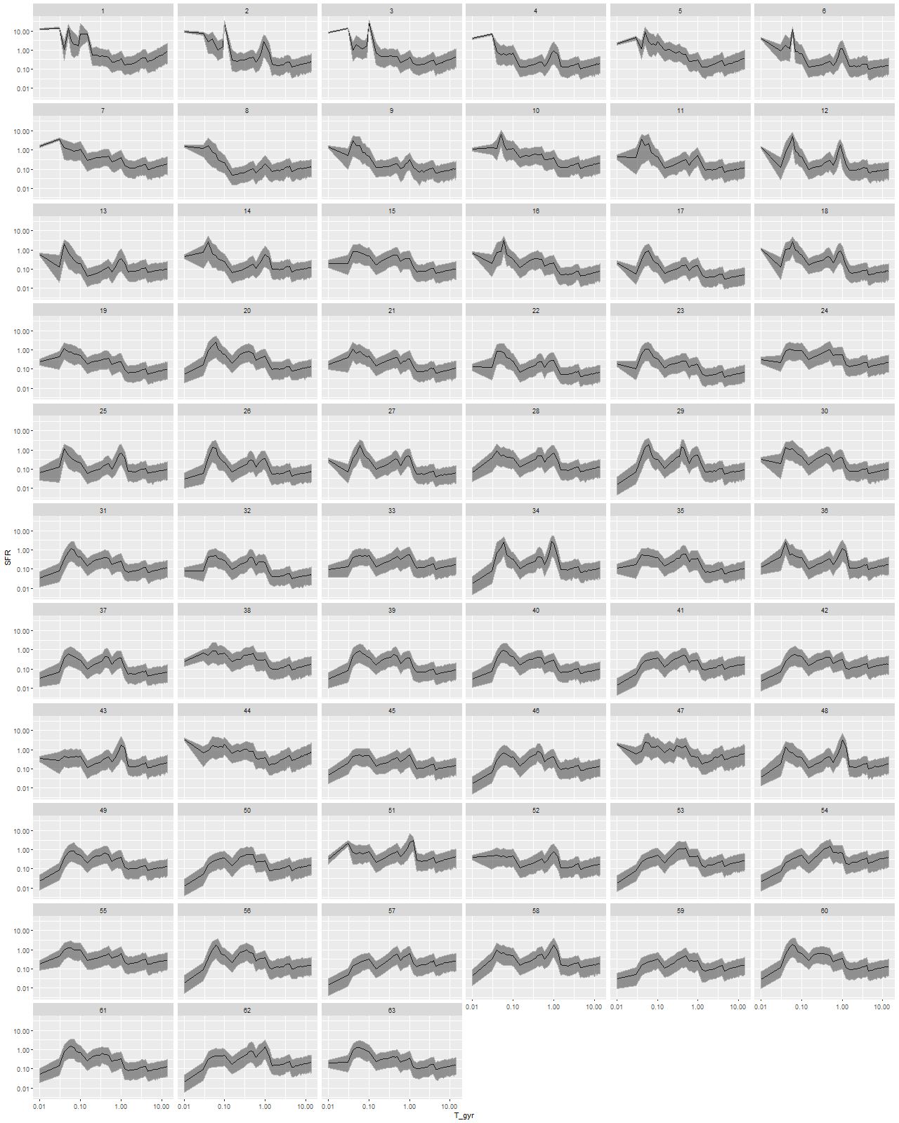
I modeled star formation histories with my largest subset of the EMILES library consisting of SSP model spectra for 54 time bins and 4 metallicity bins. As in previous exercises I fit emission lines and the stellar contribution simultaneously, which is riskier than usual in this system because some regions, especially near the northern nucleus, have complex velocity structures producing emission line profiles that are far from single component gaussians. I’ll look at this in more detail in a future post, but for now let’s just take these SFH models at face value and see where they lead. As I’ve done in several previous posts what’s plotted below are star formation rates in solar masses/year over cosmic time, counting backwards from “now” (now being when the light left the galaxies about 500Myr ago). This time I’ve used log scaling for both axes and for the first time in these posts I’ve displayed results for every bin ordered by increasing distance from the IFU center. The first two rows cover the central ~few kpc region surrounding the northern nucleus. The southern nucleus covered by bin 44 is in row 8, second from left. Both the time and SFR scales are the same for all plots. The black lines are median posterior marginal estimates and the ribbons are 95% posterior confidence intervals.
Star formation histories for the Voronoi binned regions shown in the previous map. Numbers at the top correspond to the bin numbers in the map.
Browsing through these, all regions show ∼constant or gradually decreasing star formation up to about 1 Gyr ago1You may recall I’ve previously noted there is always an uptick in star formation rate at 4 Gyr in my EMILES based models, and that’s seen in all of these as well. This must be spurious, but I still don’t know the cause.. This of course is completely normal for spiral galaxies.
Most regions covered by the IFU began to show accelerated and in some areas bursts of star formation at ∼1 Gyr. In more than half of the bins the maximum star formation rate occurred around 40-60 Myr ago, with a decline or in some areas cessation of star formation more recently. In the central few kpc around the northern nucleus on the other hand star formation accelerated rapidly beginning ~100 Myr ago and continues at high levels. The southern nucleus has a rather different estimated recent star formation history, with no (visible) starburst and instead gradually increasing SFR to a recent maximum. Ongoing star formation at measurable levels is much more localized in the southern central regions and weaker by factors of several than the northern companion.
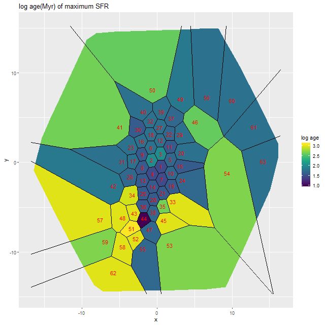
Here’s a map that I thought would be too noisy to be informative, but turns out to be rather interesting. This shows the spatial distribution of the lookback time to the epoch of maximum star formation rate estimated by the marginal posterior mean. The units displayed are log(age) in Myr; recall that I added unevolved SSP models from the 2013 update of the BC03 models to the BaSTI based SSP library, assigning them an age of 10Myr, so a value of 1 here basically means ≈ now.
Look back time to epoch of maximum star formation rate as estimated by marginal posterior mean. Units are log(age in Myr).
To summarize, there have been three phases in the star formation history of this system: a long period of normal disk galaxy evolution; next beginning about 1 Gyr ago widespread acceleration of the SFR with localized bursts; and now, within the past 50-100 Myr a rapid increase in star formation that’s centrally concentrated in the two nuclei (but mostly the northern one) while the peripheral regions have had suppressed activity.
I previously reviewed some of the recent literature on numerical studies of galaxy mergers. The high resolution simulations of Hopkins et al. (2013) and the movies available online at http://www.tapir.caltech.edu/~phopkins/Site/Movies_sbw_mgr.html seem especially relevant, particularly their Milky Way and Sbc analogs. They predict a general but clumpy enhancement of star formation at around the time of first pericenter passage; a stronger, centrally concentrated starburst at the time of second pericenter passage, with a shorter period of separation before coalescence. Surprisingly perhaps, the merger timescales for both their MW and Sbc analogs are very similar to my SFH models, with ∼ 1 Gyr between first and second perigalactic passage and another few 10’s of Myr to final coalescence.
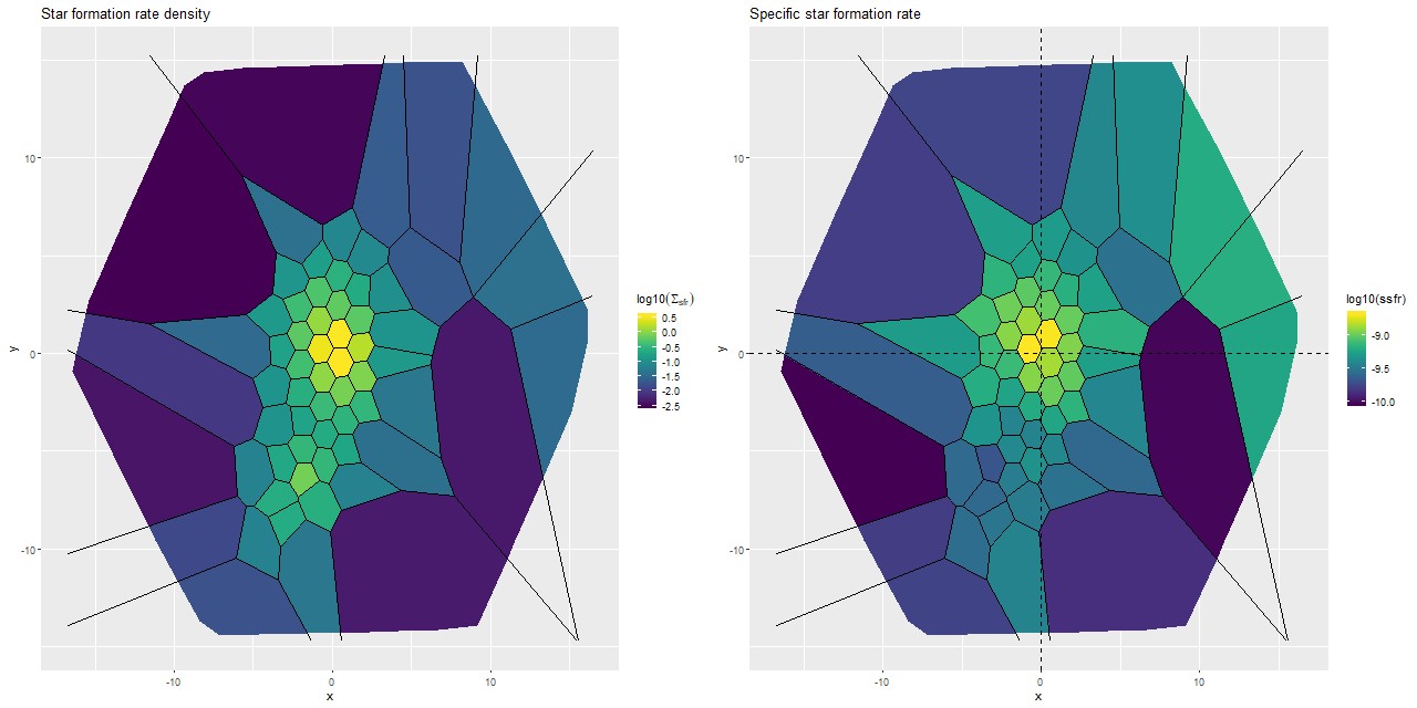
I’m going to wrap up with maps of the (posterior mean estimates) of star formation rate density (as \(\log10(\mathsf{M_\odot/yr/kpc^2})\)) and specific star formation rate, which has units log10(yr-1). These are 100Myr averages and recall are based solely on the SSP template contributions.
(L) Star formation rate density
(R) Specific star formation rate
Several recent papers have made quantitative estimates of star formation rates in this system, which I’ll briefly review. Detailed comparisons are somewhat difficult because both the timescales probed by different SFR calibrators differ and the spatial extent considered in the studies varies, so I’ll just summarize reported results and compare as best as I can.
Yuan et al. (2018) modeled broad band UV-IR SED’s taking data from GALEX, SDSS, and Spitzer; and also did full spectrum fitting using ppxf on the same MaNGA data I’ve been examining. They divided the data into 5″ (≈ 4 kpc) radius regions covering the tidal tails and each nucleus. The broadband data were fit with parametric SFH models with a pair of exponential bursts (one fixed at 13Gyr, the other allowed to vary). From the parametric models they estimated the SFR in the northern and southern nuclei as 76 and 11 \(\mathsf{M_\odot/yr}\) (the exact interpretation of this value is unclear to me). For comparison I get values of 33 and 13 \(\mathsf{M_\odot/yr}\) for regions within 4 kpc of the two nuclei by calculating the average (posterior mean) star forming density and multiplying by π*42. They also calculated 100Myr average SFRs from full spectrum fitting with several different dust models and also from the Hα luminosity, deriving estimates that varied by an order of magnitude or more. Qualitatively we reach similar conclusions that the tails had earlier starbursts and are now forming stars at lower rates than their peak, and also that the northern nucleus has recent star formation a factor of several higher than the southern.
Cluver et al. (2017) were primarily trying to derive SFR calibrations for WISE W3/W4 filters using samples of normal star forming and LIRG/ULIRGs (including this system) with Spitzer and Herschel observations. Oddly, although they tabulate IR luminosities for the entire sample they don’t tabulate SFR estimates. But plugging into their equations 5 and 7 I get star formation rate estimates of just about 100 \(\mathsf{M_\odot/yr}\). These are global values for the entire system. For comparison I get a summed SFR for my models of ≈ 45 \(\mathsf{M_\odot/yr}\) (after making a 0.2 dex adjustment for fiber overlap).
Tsai and Hwang (2015) also used IR data from Spitzer and conveniently present results for quantities I track using the same units. Their estimates of the (log) stellar mass density, SFR density, and specific star formation rate in the central kpc of (presumably) the northern nucleus were 9.85±0.09, 0.43±0.00, and -9.39±0.09 respectively. For comparison in the fiber that covers the northern nucleus my models return 9.41±0.02, 0.57±0.04, and -8.84±0.04. For the 6 fibers closest to the nucleus the average stellar mass density drops to 9.17 and SFR density to about 0.39. So, our SFR estimates are surprisingly close while my mass density estimate is as much as 0.7 dex lower.
Finally, Vega et al. (2008) performed starburst model fits to broadband IR-radio data. They estimated a burst age of about 60Myr for this system, with average SFR over the burst of 225 \(\mathsf{M_\odot/yr}\) and current (last 10 Myr) SFR 87 \(\mathsf{M_\odot/yr}\) in a starforming region of radius 0.27kpc. Their model has optical depth of 33 at 1 μm, which would make their putative starburst completely invisible at optical wavelengths. Their calculations assumed a Salpeter IMF, which would add ≈0.2 dex to stellar masses and star formation rates compared to the Kroupa IMF used in my models.
Overall I find it encouraging that my model SFR estimates are no worse than factors of several lower than what are obtained from IR data — if the Vega+ estimate of the dust optical depth is correct most of the star formation is well hidden. Next time I plan to look at Hα emission and tie up other loose ends. If time permits before I have to drop this for a while I may look at two component dust models.
This galaxy1also known as VV705, IZw 107, IRAS F15163+4255, among others has been my feature image since I started this blog. Why is that besides that it’s kind of cool looking? As I’ve mentioned before I took a shot a few years ago at selecting a sample of “transitional” galaxies from the SDSS spectroscopic sample, that is ones that may be in the process of rapidly shutting down star formation2See for example Alatalo et al. (2017) for recent usage of this terminology.. I based the selection on a combination of strong Hδ absorption and either weak emission lines or line ratios other than pure starforming, using measurements from the MPA-JHU pipeline. This galaxy pair made the sample based on the spectrum centered on the northern nucleus (there is also a spectrum of the southern nucleus from the BOSS spectrograph, but no MPA pipeline measurements). Well now, these galaxies are certainly transitioning to something, but they’re probably not shutting down star formation just yet. Simulations of gas rich mergers generally predict a starburst that peaks around the time of final coalescence. There is also significant current star formation, as high as 100-200 \(M_\odot/yr\) per various literature estimates, although it is mostly hidden. So on the face of it at least this appears to be a false positive. This was also an early MaNGA target, and one of a small number where both nuclei of an ongoing merger are covered by a single IFU:
Markarian 848. SDSS image thumbnail with MaNGA IFU footprint.
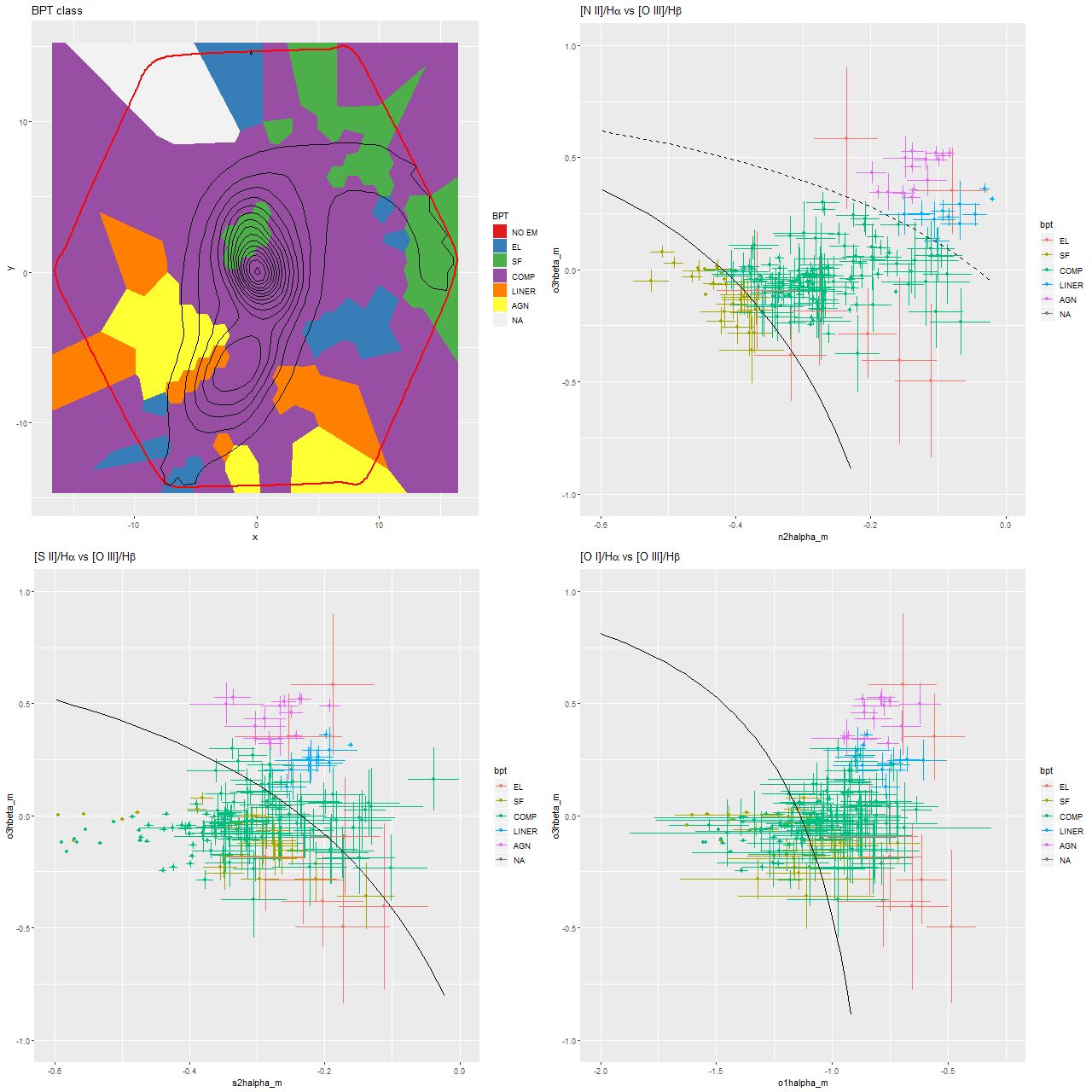
Today I’m going to look at a few results of my analysis of the IFU data that aren’t too model dependent to get some insight into why this system was selected. As usual I’m looking at the stacked RSS data rather than the data cubes, and for this exercise I Voronoi binned the spectra to a very low target SNR of 6.25. This leaves most of the fibers unbinned in the vicinity of the two nuclei. First, here is a map of BPT classification based on the [O III]/Hβ vs. [N II]/Hα diagnostic as well as scatterplots of several BPT diagnostics. Unfortunately the software I use for visualizing binned maps extends the bins out to the edge of the bounding rectangle rather than the hexagonally shaped edge of the data, which is outlined in red. Also note that different color coding is used for the scatter plots than the map. The contour lines in the map are arbitrarily spaced isophotes of the synthesized R band image supplied with the data cube.
Map of BPT class determined from [O III]/Hβ vs. [N II}/Hα diagnostic diagram, and BPT diagnostics for [N II], [S II] and [O I]. Curves are boundary lines form Kewley et al. (2006).
What’s immediately obvious is that most of the area covered by the IFU including both nuclei fall in the so-called “composite” region of the [N II]/Hα BPT diagram. This gets me back to something I’ve complained about previously. There was never a clear physical justification for the composite designation (which recall was first proposed in Kauffmann et al. 2003), and the upper demarcation line between “pure” AGN and composite systems as shown in the graph at upper right was especially questionable. It’s now known if it wasn’t at the turn of the century (which I doubt is the case) that a number of ionization mechanisms can produce line ratios that fall generally in the composite/LINER regions of BPT diagnostics. Shocks in particular are important in ongoing mergers. High velocity outflow of both ionized and neutral gas have been observed in the northern nucleus by Rupke and Veillux (2013), which they attributed to supernova driven winds.
The evidence for AGN in either nucleus is somewhat ambiguous. Fu et al. (2018) called this system a binary AGN, but that was based on the “composite” BPT line ratios from the same MaNGA data as we are examining (their map, by the way, is nearly identical to mine; see also Yuan et al. 2018). By contrast Vega et al. 2008 were able to fit the entire SED from NIR to radio frequencies with a pure starburst model and no AGN contribution at all, while more recently Dietrich et al. 2018 estimated the AGN fraction to be around 0.25 from NIR to FIR SED fitting. A similar conclusion that both nuclei contain both a starburst and AGN component was reached by Vardoulaki et al. 2015 based on radio and NIR data. One thing I haven’t seen commented on in the MaNGA data that possibly supports the idea that the southern nucleus harbors an AGN is that the regions with unambiguous AGN-like optical emission line ratios are fairly symmetrically located on either side of the southern nucleus and separated from it by ∼1-2 kpc. This could perhaps indicate the AGN is obscured from our view but visible from other angles.
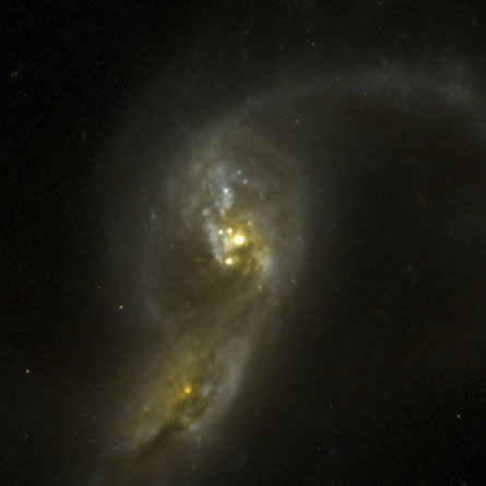
There are also several areas with starforming emission line ratios just to the north and east of the northern nucleus and scattered along the northern tidal tail (the southern tail is largely outside the IFU footprint). In the cutout below taken from a false color composite of the F435W+F814W ACS images several bright star clusters can be seen just outside the more heavily obscured nuclear region, and these are likely sources of ionizing photons.
Markarian 848 nuclei. Cutout from HST ACS F814W+F435W images.
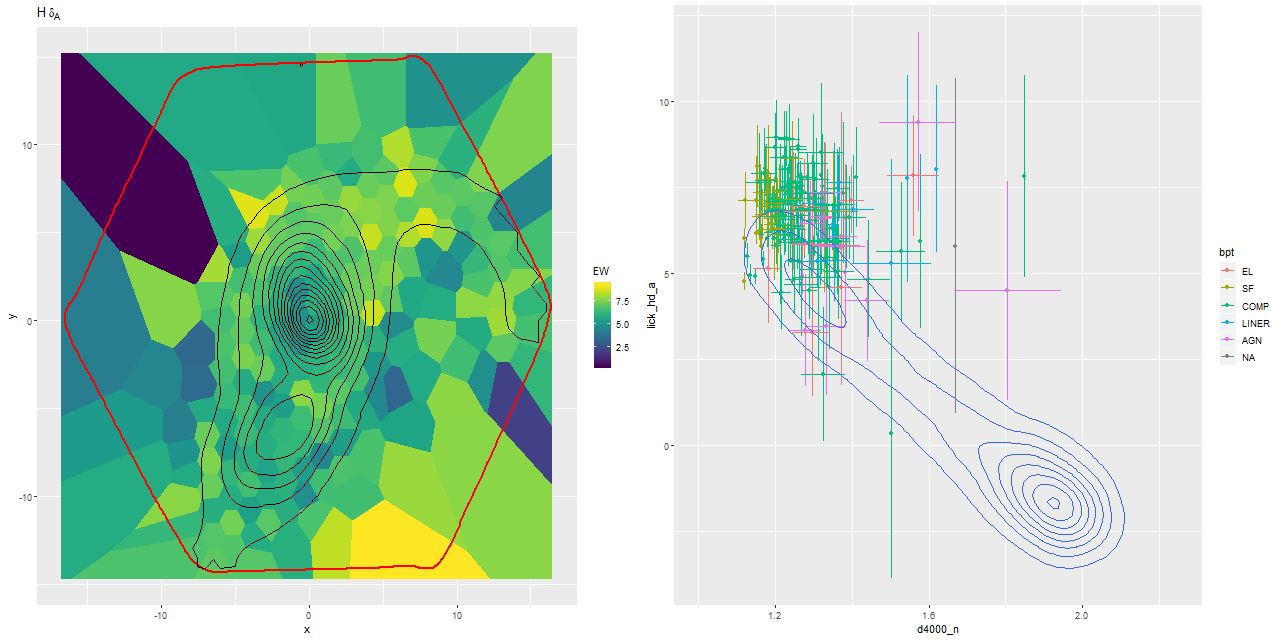
Finally turning to the other component of the selection criteria, here is a map of the (pseudo) Lick HδA index and a plot of the widely used HδA vs Dn(4000) diagnostic. It’s a little hard to see a clear pattern in the map because this is a rather noisy index, but strong Balmer absorption is seen pretty much throughout, with the highest values outside the two nuclei and especially along the northern tidal tail.
Location in the Hδ – D4000 plane doesn’t uniquely constrain the star formation history, but the contour plot taken from a largish sample of SDSS spectra from the NGP is clearly bimodal, with mostly starforming galaxies at upper left and passively evolving ones at lower right, with a long “green valley” in between. Simple models of post-starburst galaxies will loop upwards and to the right in this plane as the starburst ages before fading towards the green valley. This is exactly where most of points in this diagram lie, which certainly suggests an interesting recent star formation history.
(L) Map of HδA index.
(R) HδA vs Dn(4000) index. Contours are for a sample of SDSS spectra from the north galactic pole.
I’m going to end with a bit of speculation. In simulations of gas rich major mergers the progenitors generally complete 2 or 3 orbits before final coalescence, with some enhancement of star formation during the perigalactic passages and perhaps some ebbing in between. This process plays out over hundreds of Myr to some Gyr. What I think we are seeing now is the 2nd or third encounter of this pair, with the previous encounters having left an imprint in the star formation history.
I’ve done SFH modeling for this binning of the data, and also for data binned to higher SNR and modeled with higher time resolution models. Next post I’ll look at these in more detail.
This post has been languishing in draft form for well over a month thanks to travel and me losing interest in the subject. I’m going to try to get it out of the way quickly and move on.
Last time I noted the presence of apparent outliers in the relationship between stellar mass and rotation velocity and pointed out that most of them are due to model failures of various sorts rather than “cosmic variance.” That would seem to suggest the need for some sample refinement, and the question then becomes how to trim the sample in a way that’s reproducible.
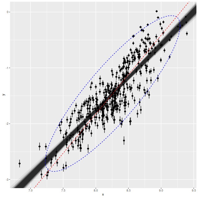
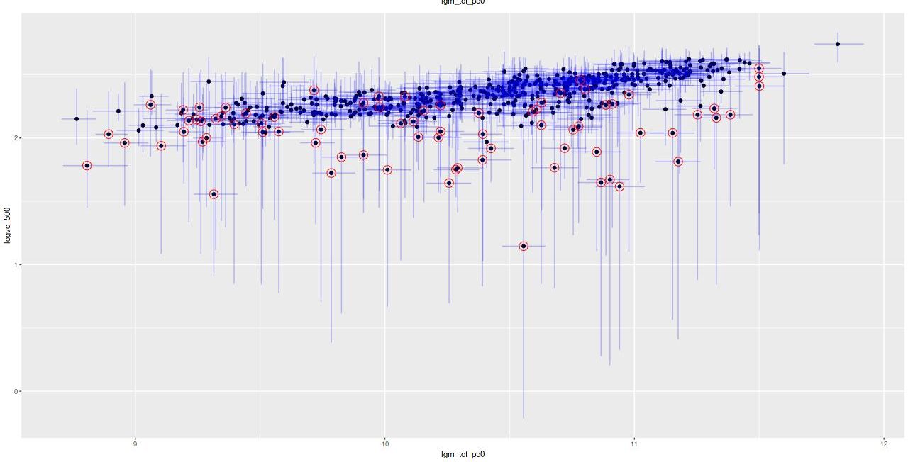
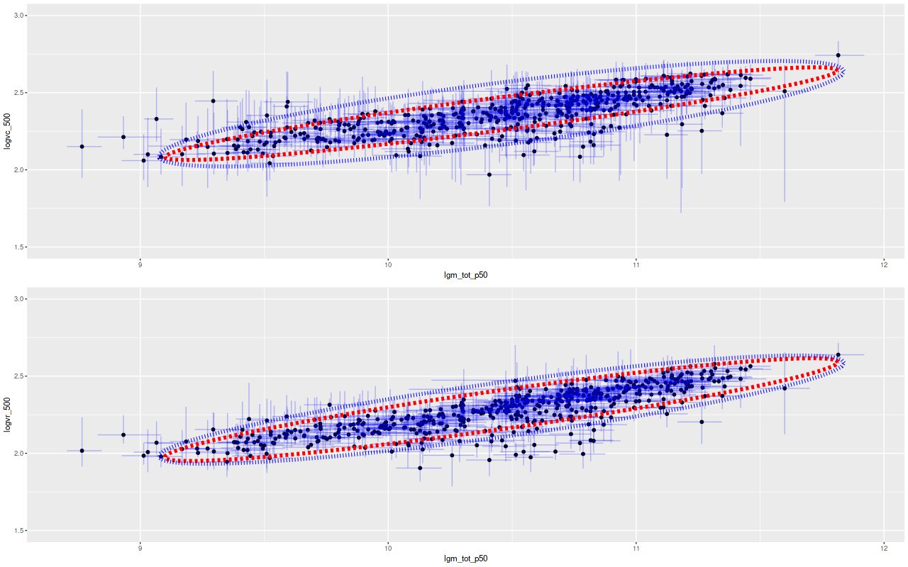
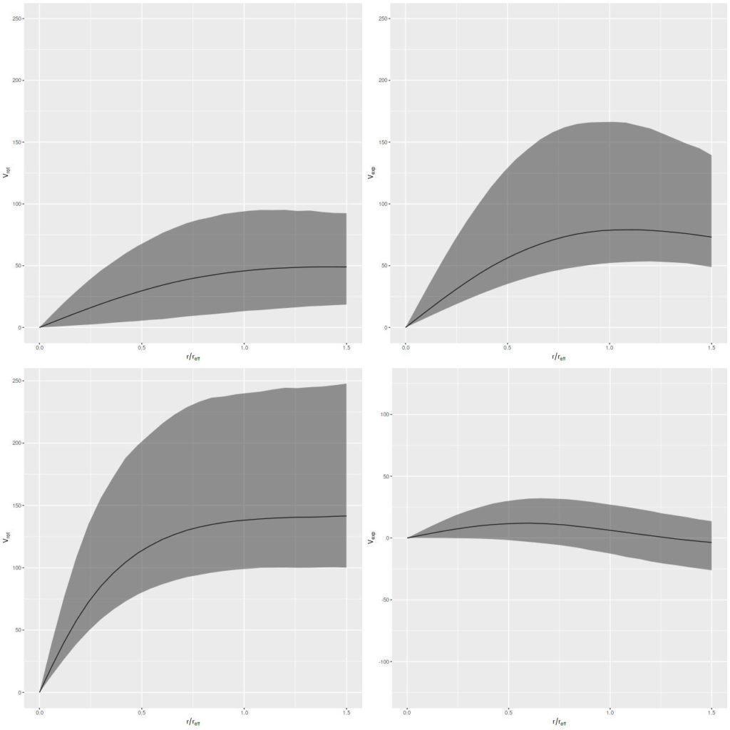
An obvious comment is that all of the outliers fall below the general trend and (less obviously perhaps) most have very large posterior uncertainties as well. This suggests a simple selection criterion: remove the measurements which have a small ratio of posterior mean to posterior standard deviation of rotation velocity. Using the asymptotic circular velocity v_c in the atan mean function and setting the threshold to 3 standard deviations the sample members that are selected for removal are circled in red below. This is certainly effective at removing outliers but it’s a little too indiscriminate — a number of points that closely follow the trend are selected for removal and in particular 19 out of 52 points with stellar masses less than \(10^{9.5} M_\odot\) are selected. But, let’s look at the results for this trimmed sample.
Posterior distribution of asymptotic velocity `v_c` vs stellar mass. Circled points have posterior mean(v_c)/sd(v_c) < 3.
Again I model the joint relationship between mass and circular velocity using my Stan implementation of Bovy, Hogg, and Roweis’s “Extreme deconvolution” with the simplification of assuming gaussian errors in both variables. The results are shown below for both circular velocity fiducials. Recall from my previous post on this subject the dotted red ellipse is a 95% joint confidence interval for the intrinsic relationship while the outer blue one is a 95% confidence ellipse for repeated measurements. Compared to the first time I performed this exercise the former ellipse is “fatter,” indicating more “cosmic variance” than was inferred from the earlier model. I attribute this to a better and more flexible model. Notice also the confidence region for repeated measurements is tighter than previously, reflecting tighter error bars for model posteriors.
Joint distribution of stellar mass and velocity by “Extreme deconvolution.” Inner ellipse: 95% joint confidence region for the intrinsic relationship. Outer ellipse: 95% confidence ellipse for new data.
Top: Asymptotic circular velocity v_c.
Bottom: Circular velocity at 1.5 r_eff.
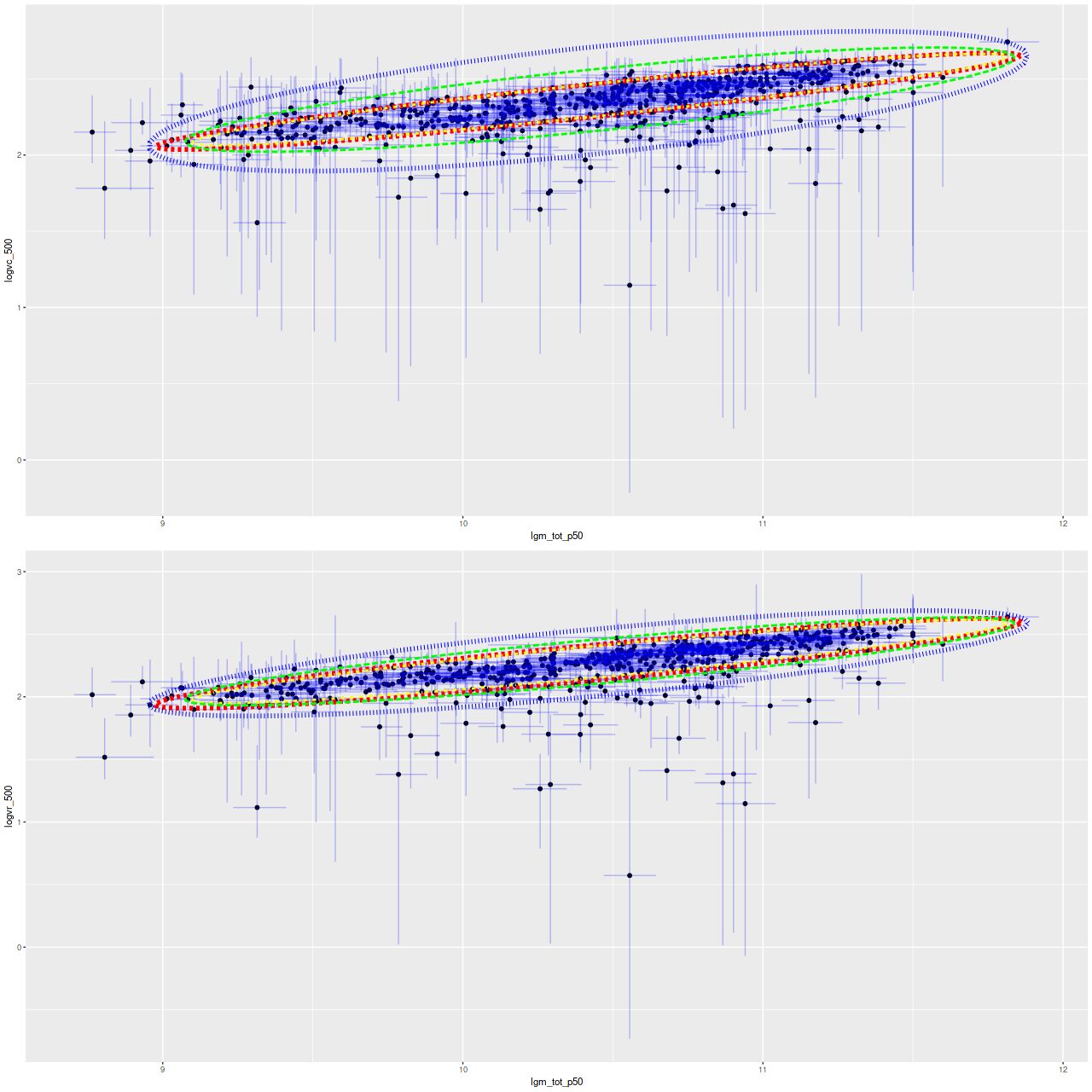
Now here is something of a surprise: below are the model results for the full sample compared to the trimmed one. The red and yellow ellipses are the estimated intrinsic relations using the full and trimmed samples, while green and blue are for repeated measurements. The estimated intrinsic relationships are nearly identical despite the many outliers. So, even though this model wasn’t formulated to be “robust” as the term is usually understood in statistics in practice it is, at least as regards to the important inferences in this application.
Joint distribution of stellar mass and velocity by “Extreme deconvolution” (complete sample). Inner ellipse: 95% joint confidence region for the intrinsic relationship. Outer ellipse: 95% confidence ellipse for new data. Top: Asymptotic circular velocity v_c. Bottom: Circular velocity at 1.5 r_eff.
Finally the slope, that is the exponent in the stellar mass Tully-Fisher relationship \(M^* \sim V_{rot}^\gamma\) is estimated as the (inverse of) slope of the major axis of the inner ellipses in the above plots. The posterior mean and 95% marginal confidence intervals for the two velocity measures and both samples are:
v_c (subset 1) \(4.81^{+0.28}_{-0.25}\)
v_c (all) \(4.81^{+0.28}_{-0.25}\)
v_r (subset 1) \(4.36^{+0.23}_{-0.20}\)
v_r (all) \(4.33^{+0.23}_{-0.21}\)
Does this suggest some tension with the value of 4 determined by McGaugh et al. (2000)? Not necessarily. For one thing this is properly an estimate of the stellar mass – velocity relationship, not the baryonic one. Generally lower stellar mass galaxies will have higher gas fractions than high stellar mass ones, so a proper accounting for that would shift the slope towards lower values. Also, and as can be seen here, both the choice of fiducial velocity and analysis method matter. This has been discussed recently in some detail by Lelli et al. (2019)1These two papers have two authors in common..
Next time, back to star formation history modeling.
Last time I left off with the remark that while most of the sample of disk galaxies clearly exhibits a tight relationship between circular velocity and stellar mass, there are some apparent outliers as well. While some “cosmic variance” is expected most of the apparent outliers are due to model failures, which have several possible causes:
Violation of the physical assumptions of the model, namely that the stars and gas are rotating (together) in the plane of a thin disk that’s moderately inclined to our line of sight (see my original post on this topic).
Errors in the photometry. I use two photometric quantities (specifically nsa_elpetro_ba and nsa_elpetro_phi) from the MaNGA DRPALL catalog to set priors for the kinematic parameters cos_i and phi(cosine of the disk inclination and angle to receding side) and also to initialize the sampler. Since proper and in practice fairly informative priors are required for these parameters errors here will propagate into the models, sometimes in ways that are fatal. I’ll look in more detail at some examples below.
Bad velocity data.
Not enough data.
Sampler convergence failures with no obvious cause.
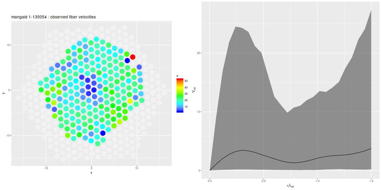
The first two bullet points are closely related: most of the failures to satisfy the physical assumptions are directly related to errors in the photometric decompositions. One fairly common failure was galaxies that were too nearly face on to obtain reliable rotation curves. As an example here is the galaxy with the lowest estimated rotation velocity in the sample, mangaid 1-135054 (plateifu 8550-12703):
Mangaid 1-135054 (plateifu 8550-12703). (L) Measured velocity field and (R) posterior predictive estimate of circular velocity with 95% confidence band.
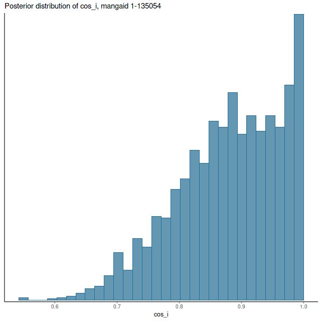
Besides showing no sign of rotation the velocity field hints at possible large scale, low velocity outflow in the central region. There are also a few apparent outliers, although these had little effect on model results. Fortunately the model output gives us plenty of clues that the results shouldn’t be trusted. The median circular velocity estimate is unrealistically low with very large posterior uncertainty (above right), while the posterior marginal density for cos_ihas a mode near 1 and also very large uncertainty (below).
Mangaid 1-135054 (plateifu 8550-12703). Posterior distribution of cosine of disk inclination.
Zooming out a bit on SDSS imaging gives a likely explanation for the peculiar velocity field. The elliptical galaxy just to the NW has nearly the same redshift (the velocity difference is ∼75 km/sec) and is almost certainly interacting with our target.
MaNGA target and companion; credit SDSS
A key assumption in using photometric properties as proxies for kinematic quantities is that disk galaxies have intrinsically circular surface brightness profiles. This is never quite the case in practice and sometimes morphological features like strong bars can make this assumption catastrophically wrong. Here was perhaps the most extreme example in DR14:
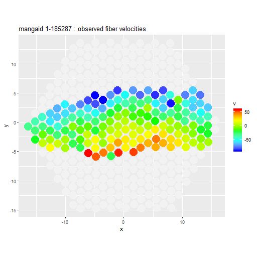
mangaid 1-185287 (plateifu 8252-12704). SDSS thumbnail with IFU overlay
mangaid 1-185287 (plateifu 8252-12704) Measured velocity field from stacked RSS spectra
The photometric major axis angle was estimated to be 98.4o, that is just south of east, while the position angle of the maximum recession velocity is close to due south. When I first examined this velocity field I had a hard time reconciling it with rotation in a thin disk. This was before I learned how to do Voronoi binning though. The image below shows the binned velocity field (with a target S/N of 6.25). This shows that the relative velocity does increase on a roughly north to south line, indicating that this is indeed a rotating disk galaxy.
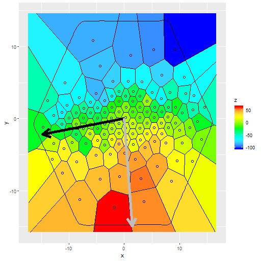
mangaid 1-185287 (plateifu 8252-12704) Measured velocity field from binned RSS spectra. Black arrow indicates major axis position angle from photometry. Gray arrow: position angle of receding side from velocity model with prior guess of 180o
I mentioned in an earlier post that without a proper prior on the kinematic position angle phi these models are inherently multi-modal (in fact they are infinitely modal and therefore would have improper posteriors). The solution to that of course is to have a proper prior. But if the prior is seriously in error the posterior estimates for the components of the velocity will end up scrambled as can be seen in the top row of the graph below, which shows the posterior distributions of the circular and “expansion” velocities1Remember that the photometric position angle is determined modulo π while the direction to the maximum recession velocity is measured modulo 2π. We don’t care about a π radian error in the prior though because that just flips the signs of the velocity components, which causes no sampling issues and is trivially fixable in the generated quantities block. It’s smaller errors that cause problems.
The obvious solution to a bad prior is to correct it2Using the data you’re trying to model to establish a prior is, technically, cheating (the polite term is “Empirical Bayes”), but this seems a relatively benign use of the data., which is easy enough. The bottom row shows the results of re-running the model with a prior phicentered on 180o and the same data. Now both the circular and expansion velocity curves are at least plausible. The posterior mean of phiis ≈185o, which is very close to correct as can be seen in the binned velocity field shown above.
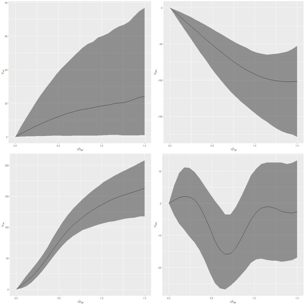
mangaid 1-185287 (plateifu 8252-12704) Top row: model rotation (L) and expansion (R) velocities with prior for major axis angle taken from photometry (phi = 98.4). Bottom row: same but with prior phi = 180o.
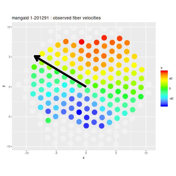
One more example. Bars were the most common cause of misleading photometric decompositions, but not the only one. Some galaxies are just asymmetrical. Here is the one that had the largest offset between the photometric and kinematic position angles:
And the velocity field (again this agrees well with the Marvin measurements of the data cube):
mangaid 1-201291 (plateifu 8145-6103). Velocity field from stacked RSS spectra with major axis angle from nsa_elpetro_phi
This time the velocity field looks unremarkable, but again because of the prior the estimated circular and expansion velocities are scrambled together. And once again also, changing the prior to be centered on the approximate actual position angle of the receding side produces reasonable estimates for both:
mangaid 1-201291 (plateifu 8145-6103). Top: Posterior predictive distributions of circular and expansion velocity with prior on `phi` from photometry. Bottom: Same with prior centered on -10o
Next up, I’ll take a more holistic look at final sample selection, and maybe get to results.
As I mentioned in the previous two posts SDSS Data Release 15 went public back in December and a query for “normal” disk galaxies as judged by Galaxy Zoo 2 classifiers returned 588 hits. I’ve finally run the GP velocity models on all of the new data and made a second run on around 40 that were contaminated by foreground stars or neighboring galaxies. So far I haven’t found an alternative to selecting these by eye and doing the masking manually, so that’s an error prone process. The month+ long gap between postings by the way was due to travel — my computer wasn’t grinding away on these models for all that time. As I mentioned last post the sampling properties including execution time of the GP model with arctangent mean function are usually quite favorable using Stan. The median wall time for these runs was about a minute, with a range from 25 to 1600 seconds. All model runs used 500 warmup iterations and 500 post-warmup with 4 chains run in parallel. This is more than enough for inference.
Before I discuss the results I’ll show them. As I did for the first pass at this way back in July I retrieved stellar mass and uncertainty estimates made by the MPA-JHU group from CasJobs; all but a handful also have mass estimates from the Wisconsin group. I may look at those later but don’t anticipate any very significant differences.
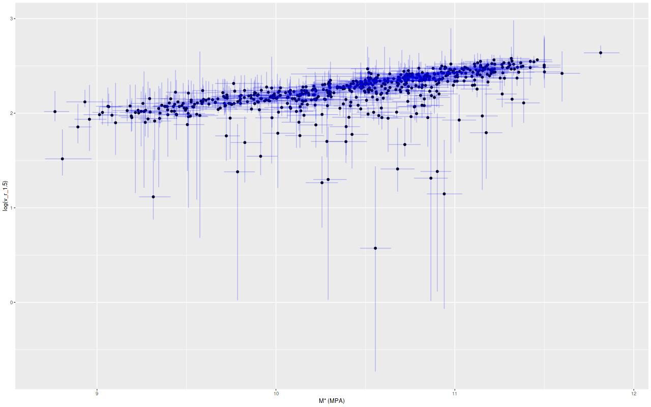
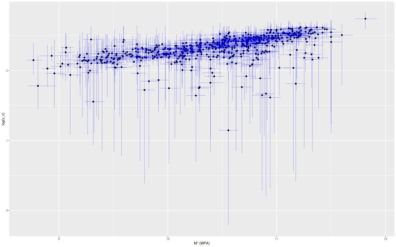
There are now at least two plausible choices for reference circular velocities: the velocity at a fiducial radius, and again I choose 1.5 effective radii since the MaNGA IFUs are meant to cover out to that radius in the primary sample. The other obvious choice is the asymptotic velocity vc in the arctangent mean function. This seems in principle to be the better choice since it estimates the circular velocity in the flat part of the rotation curve, but it might be a considerable extrapolation from the actual data in some cases.
Both sets of results are shown below for all model runs that ran to completion (N=582). Plotted are the median, 2.5, and 97.5 percentiles (≈ ± 2σ) of posterior predictions for the log-circular velocity at 1.5reff (top graph) and the same quantiles of the posteriors of the parameter v_c (bottom graph). These are plotted against the median, 16, and 84 percentiles (≈ ± 1σ) of the total stellar mass estimates per the MPA group.
Estimated rotation velocity at 1.5 effective radii vs. stellar mass estimate from MPA-JHU models
Estimated asymptotic rotation velocity against stellar mass from MPA-JHU models. Vertical error bars mark the 2.5 and 97.5 percentiles of the model posteriors of (log) velocity in km/sec. Horizontal error bars mark the 16 and 84 percentiles model posteriors of (log) stellar mass.
Evidently most of the sample follows a tight linear relationship with either measure of circular velocity, but there are some apparent outliers as well. I’m feeling a bit blocked right now, so I’ll end the post here. Next time I’ll look at some of the causes of model failure, what to do about them, and get to the results.