
This post has been languishing in draft form for well over a month thanks to travel and me losing interest in the subject. I’m going to try to get it out of the way quickly and move on.
Last time I noted the presence of apparent outliers in the relationship between stellar mass and rotation velocity and pointed out that most of them are due to model failures of various sorts rather than “cosmic variance.” That would seem to suggest the need for some sample refinement, and the question then becomes how to trim the sample in a way that’s reproducible.
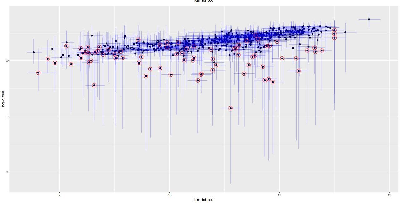
An obvious comment is that all of the outliers fall below the general trend and (less obviously perhaps) most have very large posterior uncertainties as well. This suggests a simple selection criterion: remove the measurements which have a small ratio of posterior mean to posterior standard deviation of rotation velocity. Using the asymptotic circular velocity v_c in the atan mean function and setting the threshold to 3 standard deviations the sample members that are selected for removal are circled in red below. This is certainly effective at removing outliers but it’s a little too indiscriminate — a number of points that closely follow the trend are selected for removal and in particular 19 out of 52 points with stellar masses less than \(10^{9.5} M_\odot\) are selected. But, let’s look at the results for this trimmed sample.
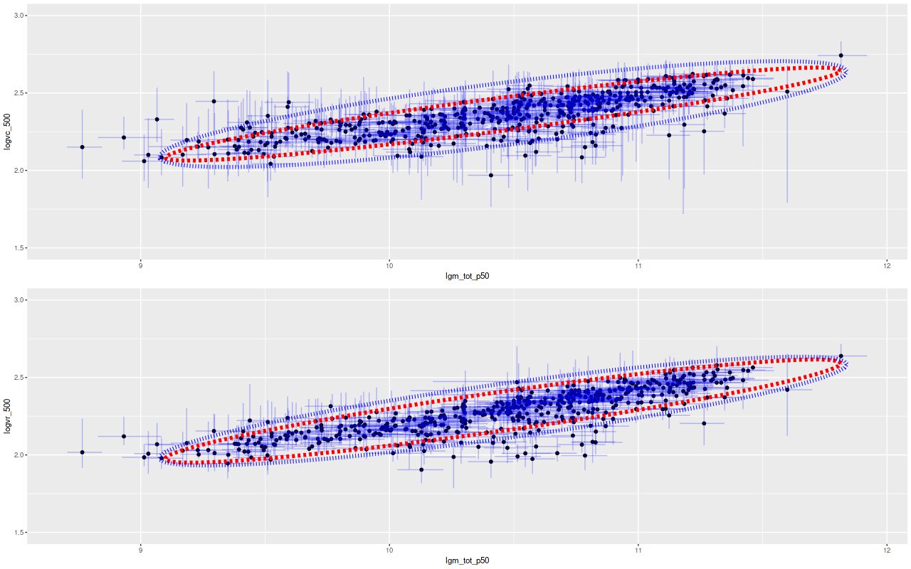
Again I model the joint relationship between mass and circular velocity using my Stan implementation of Bovy, Hogg, and Roweis’s “Extreme deconvolution” with the simplification of assuming gaussian errors in both variables. The results are shown below for both circular velocity fiducials. Recall from my previous post on this subject the dotted red ellipse is a 95% joint confidence interval for the intrinsic relationship while the outer blue one is a 95% confidence ellipse for repeated measurements. Compared to the first time I performed this exercise the former ellipse is “fatter,” indicating more “cosmic variance” than was inferred from the earlier model. I attribute this to a better and more flexible model. Notice also the confidence region for repeated measurements is tighter than previously, reflecting tighter error bars for model posteriors.
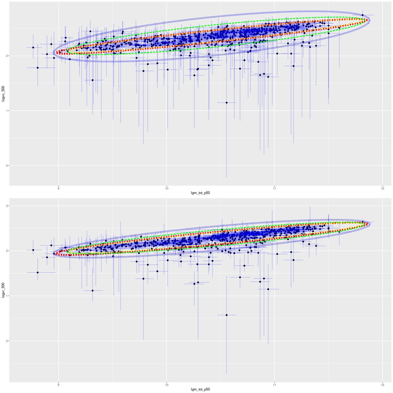
Now here is something of a surprise: below are the model results for the full sample compared to the trimmed one. The red and yellow ellipses are the estimated intrinsic relations using the full and trimmed samples, while green and blue are for repeated measurements. The estimated intrinsic relationships are nearly identical despite the many outliers. So, even though this model wasn’t formulated to be “robust” as the term is usually understood in statistics in practice it is, at least as regards to the important inferences in this application.
Finally the slope, that is the exponent in the stellar mass Tully-Fisher relationship \(M^* \sim V_{rot}^\gamma\) is estimated as the (inverse of) slope of the major axis of the inner ellipses in the above plots. The posterior mean and 95% marginal confidence intervals for the two velocity measures and both samples are:
v_c (subset 1) \(4.81^{+0.28}_{-0.25}\)
v_c (all) \(4.81^{+0.28}_{-0.25}\)
v_r (subset 1) \(4.36^{+0.23}_{-0.20}\)
v_r (all) \(4.33^{+0.23}_{-0.21}\)
Does this suggest some tension with the value of 4 determined by McGaugh et al. (2000)? Not necessarily. For one thing this is properly an estimate of the stellar mass – velocity relationship, not the baryonic one. Generally lower stellar mass galaxies will have higher gas fractions than high stellar mass ones, so a proper accounting for that would shift the slope towards lower values. Also, and as can be seen here, both the choice of fiducial velocity and analysis method matter. This has been discussed recently in some detail by Lelli et al. (2019)1These two papers have two authors in common..
Next time, back to star formation history modeling.