One thing I found odd about the 2 papers on PSB galaxies by Leung et al. that I’ve used to draw a (probably) final sample is they did no spatially resolved analyses at all, despite the fact their spectroscopic data came from MaNGA. Instead they simply summed all spectra meeting their PSB criteria, calculating a single model star formation history for each galaxy. Recently a paper by the same group showed up on arxiv (2602.13114) that begins to address the issue of spatial variations using what they refer to as a bayesian hierarchical model applied in multiple stages to Voronoi binned spectral cubes. Their approach differs in significant ways from mine: in particular they assign functional forms to the mean behavior of all parameters of their model, so for example the stellar mass density is assumed (on average) to follow a Sersic law. If I understand what they’re doing this will hugely increase the amount of data to be processed in a single model run compared to analyzing each binned spectrum separately. It likely also complicates the geometry of the model and more than proportionately increases execution time. Although they mention no timings the fact that only 3 galaxies were studied in this preliminary paper seems a clue that considerable computational resources were required. Another problem with their approach is it can’t generalize. In particular a small but nontrivial fraction of their sample are clear mergers or varyingly disturbed merger remnants. As we saw in the previous three posts these can have quite complex spatial variations in physical properties.
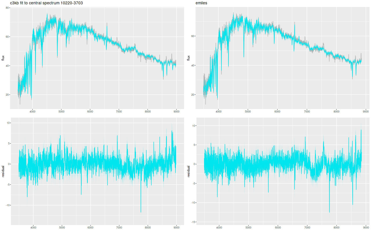
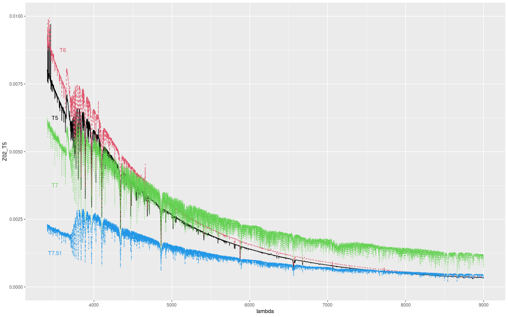
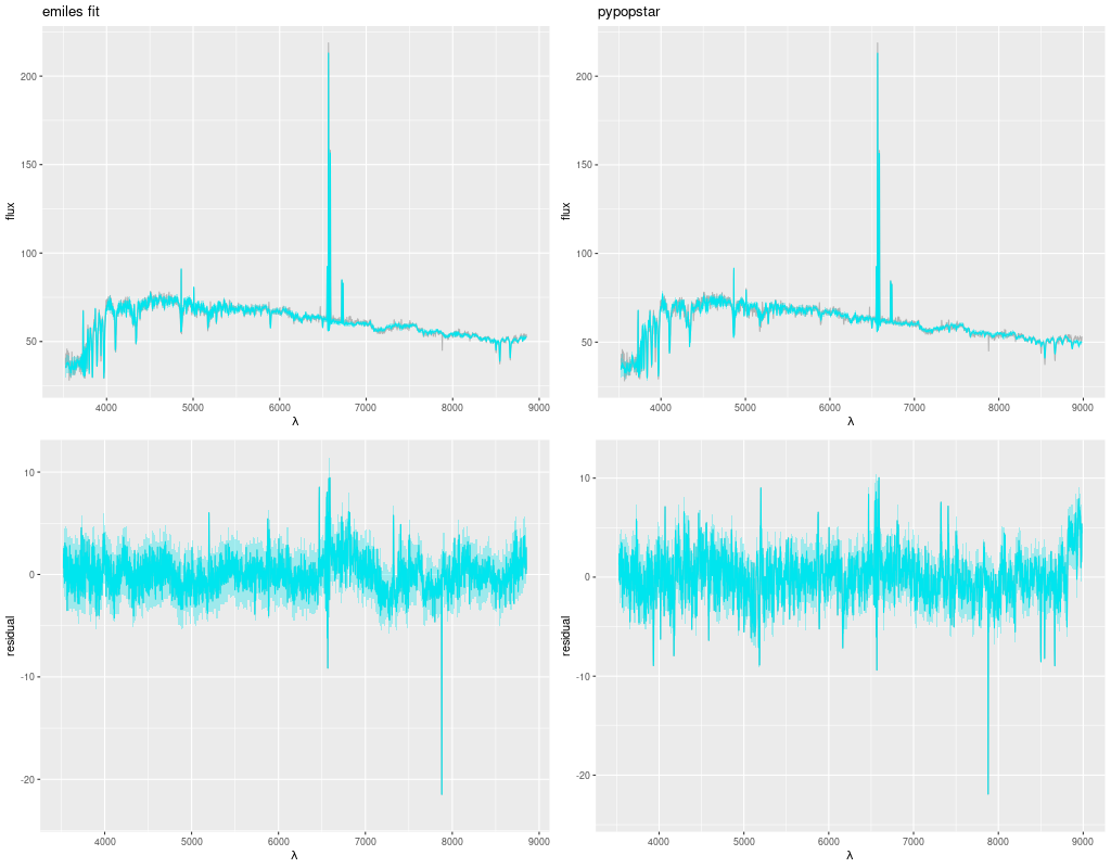
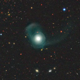
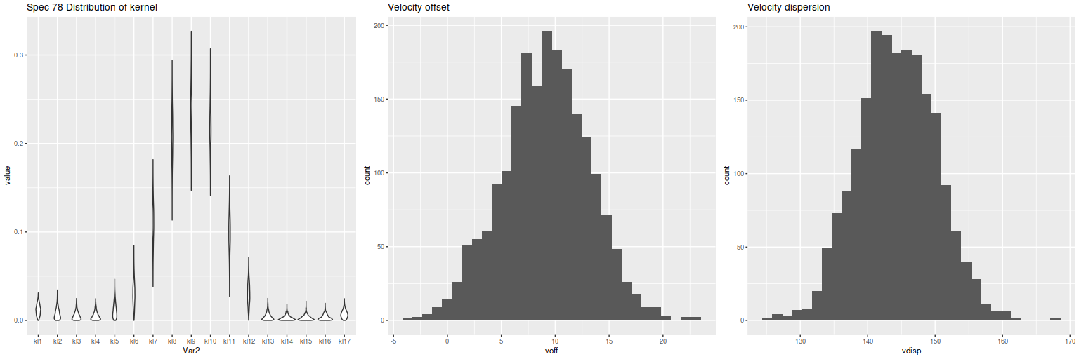
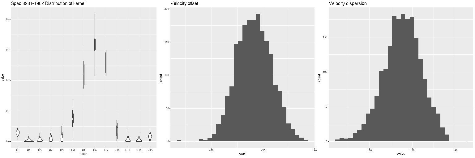
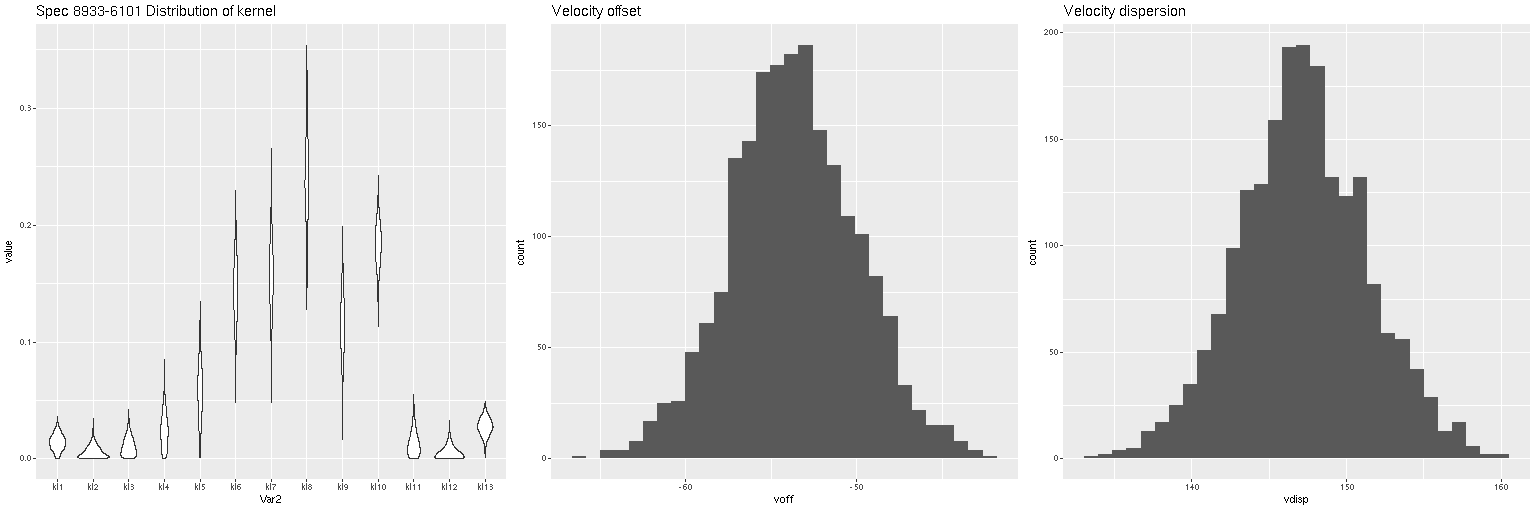
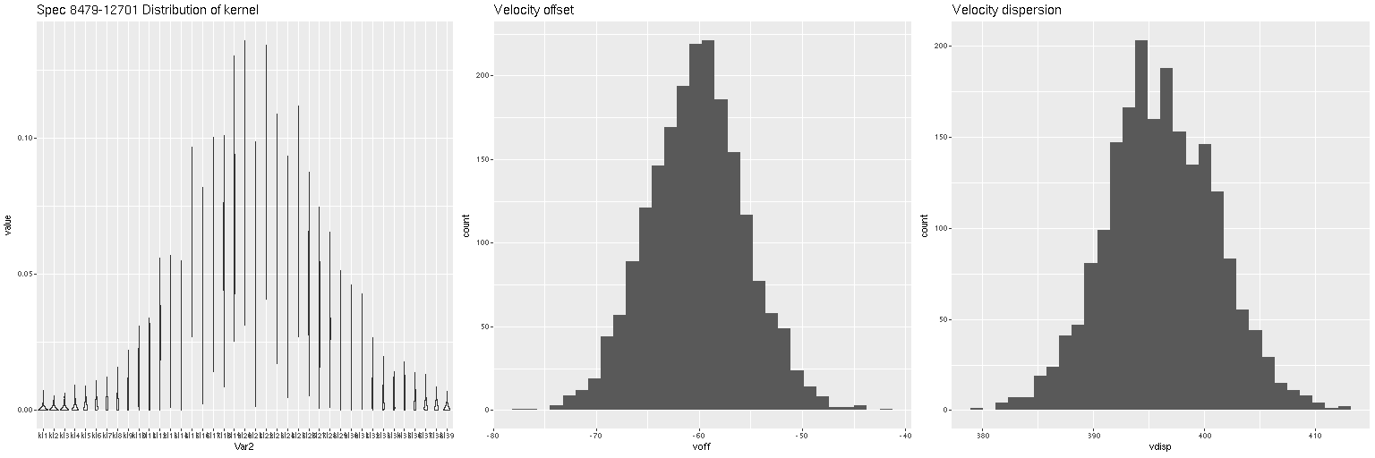
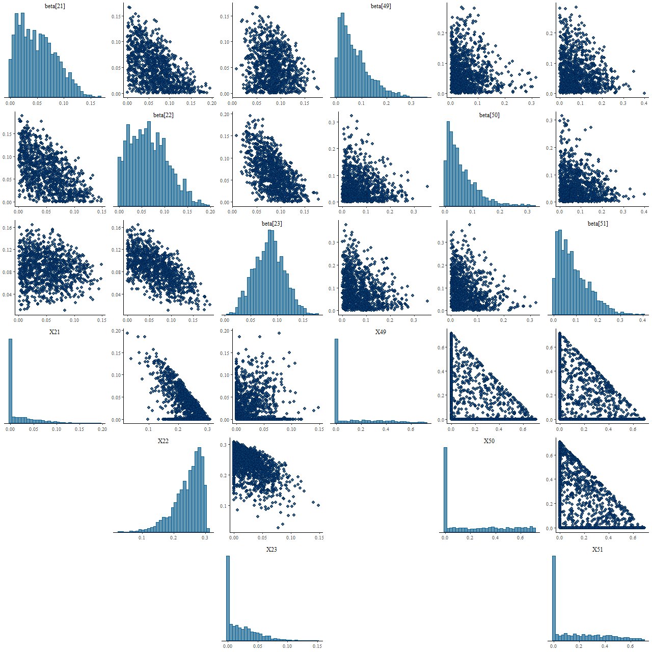
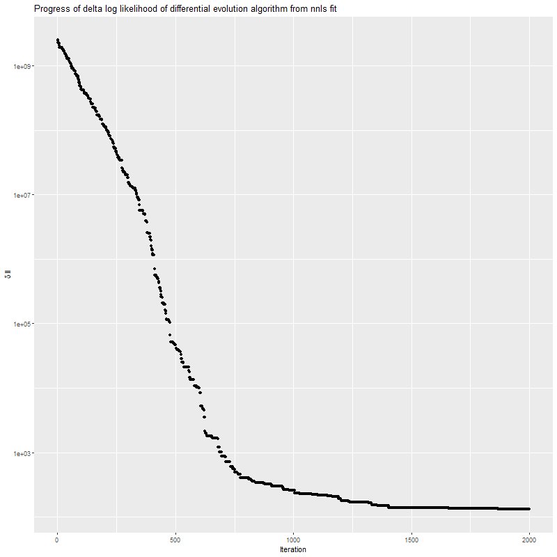
Their models do track some quantities that I also calculate, so it’s worth doing at least a semi-quantitative comparison. I picked just one of their sample for analysis: MaNGA plateifu 7965-1902 (mangaid 1-635485), aka CGCG 375-016. This is an S0 galaxy and a known post-starburst (eg Pracy et al. 2013, who also performed IFU observations). The main reason for the selection was that I was traveling at the time with only a laptop and this set of observations used the smallest 19 fiber science IFU. After binning the RSS file I obtained 52 spectra with SNR > 8. Despite the fact my laptop is mid-range and was bought on clearance at that it worked surprisingly well on this dataset, requiring only about 4 1/2 hours of total sampling time. This was probably at least partly due to the fact that its CPU has 14 cores so I was able to run with 3 threads per chain with a bit of headroom for other tasks.
I’m only going to look at a few quantities derived from the models that can be compared to Leung et al. results.
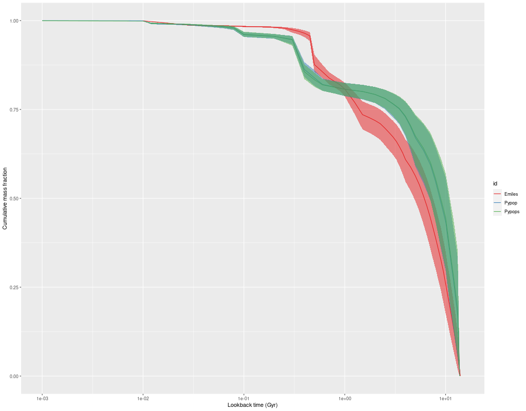
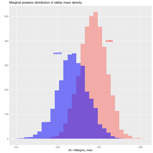
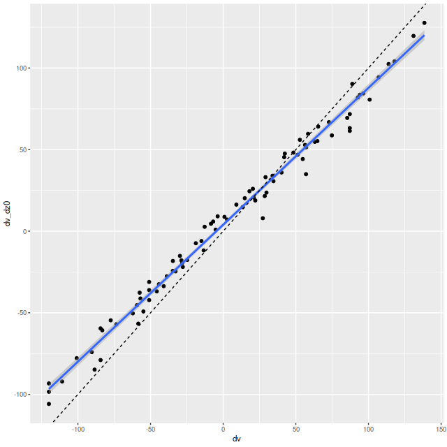
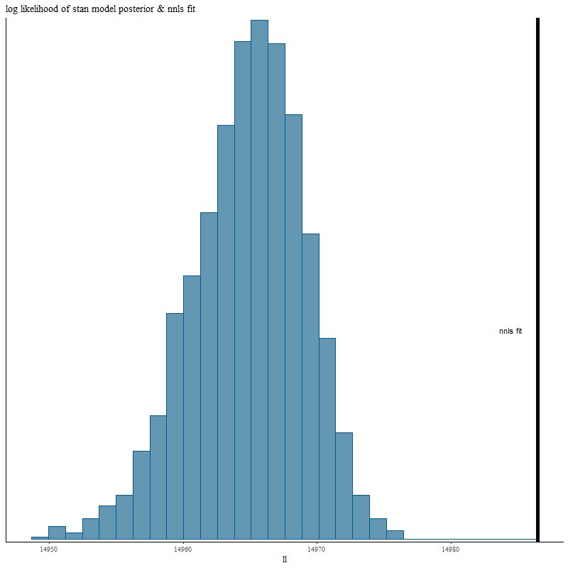
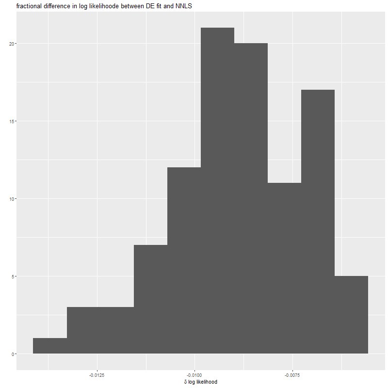
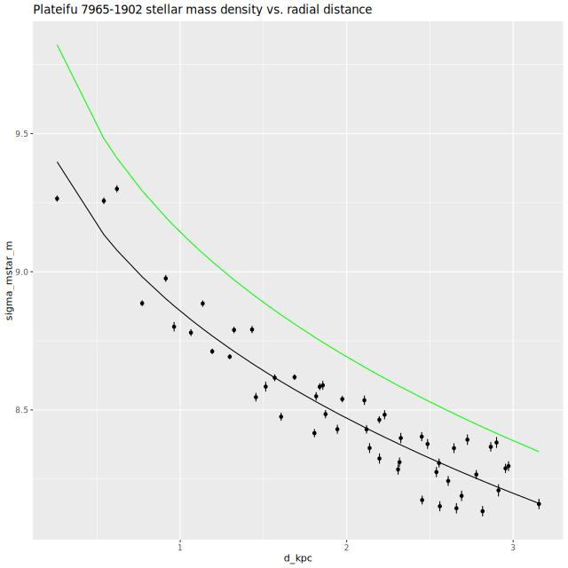
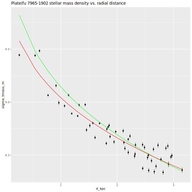
Estimates of present day stellar mass densities are a standard part of my post-processing workflow1the model parameters are simply the contributions of each SSP input model scaled to be approximately fractional light contributions at, roughly, V to the unattenuated light. All derived quantities are generated in post-processing and aren’t part of the model as such. I do most of that in R, although some is done in the “generated quantities” block of the Stan program. . The left hand plot below shows mean estimates of the stellar mass density against projected distance in kiloparsecs from the center. Leung et al. assumed a Sersic relation for the mean, which is shown as the green curve in the plot. I just did an ordinary nonlinear least squares fit to the posterior means, shown as the black line. At first sight the ≈0.2 dex systematic offset seemed a bit concerning, especially since we used the same cosmological parameters and the same stellar IMF (different libraries though). But, a recheck of the manuscript shows (section 4.3.1) that they were estimating the total stellar mass formed, which doesn’t account for mass loss over the lifetime of a SSP. That’s an easy enough calculation to perform, and the revised relation is shown on the right below. Their mean relation has a slightly steeper profile, which is likely due to differences in stellar attenuation estimates — they estimate a higher central attenuation value than I do and use a “greyer” attenuation curve, which requires a higher stellar mass density to produce the observed amount of light.
Perhaps the most significant parameters in their model are the burst age and burst strength. Neither of these are parameters of my model and there isn’t really an unambiguous way to estimate them. What I typically see in post-starbursts is a ramp up to a maximum SFR, a possible plateau with, perhaps, multiple peaks, followed by a more or less rapid decay. The beginning of the ramp up doesn’t necessarily mark the beginning of the burst — in fact it’s most likely an upper limit. Recall from my suite of simulations that the model burst typically began earlier and ramped up more gradually than the input.
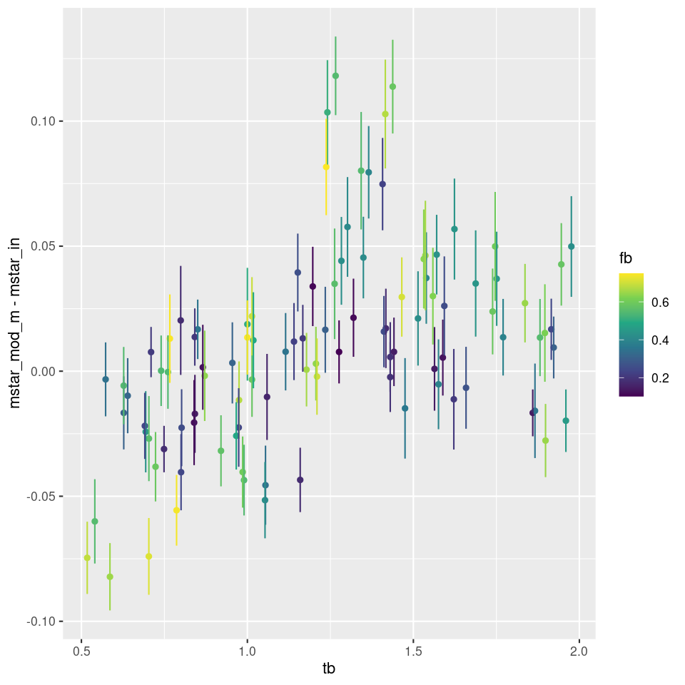
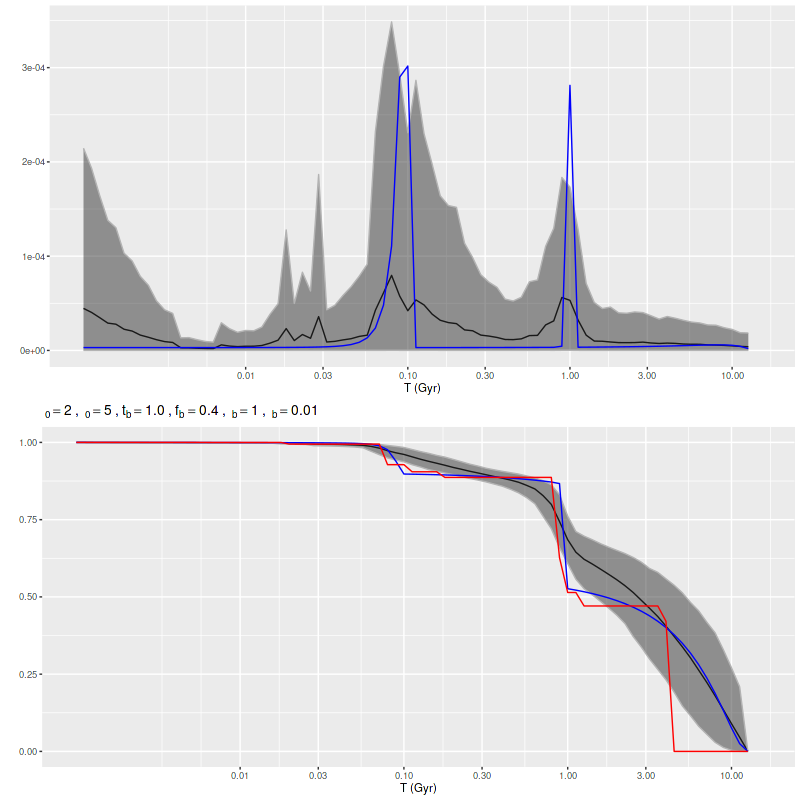
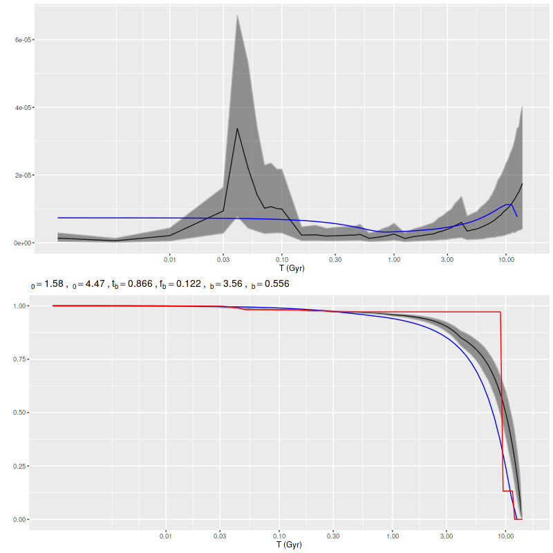
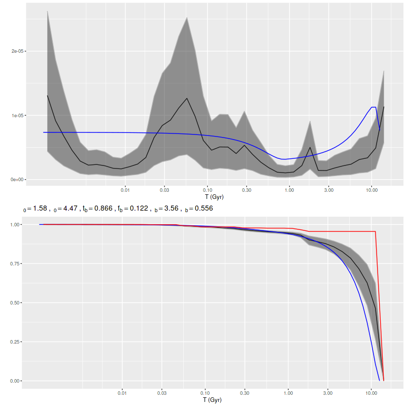
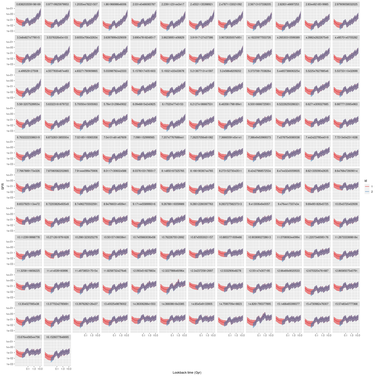
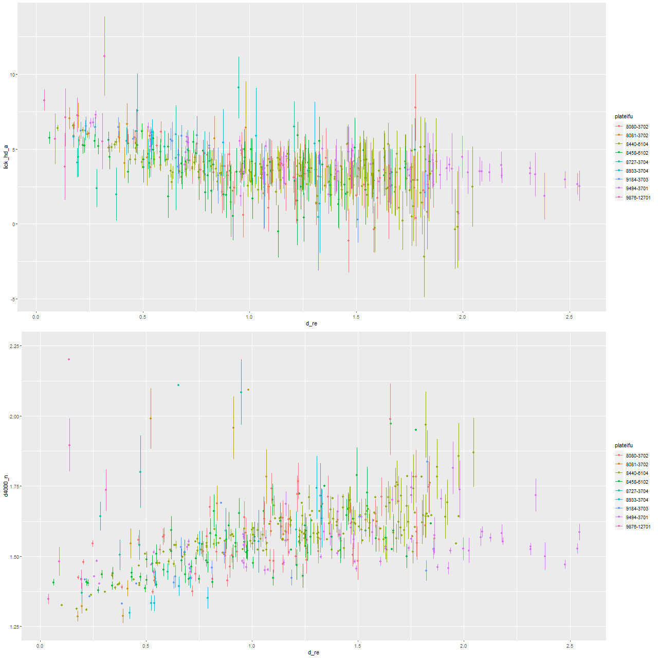
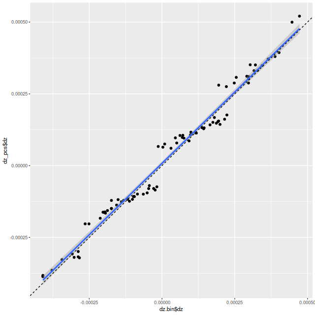
What I can measure unambiguously is the lookback time to the epoch of maximum star formation rate (per the model of course, which may well be biased), so I’ve added that to my post-processing workflow. Below I plot the lookback time to maximum SFR against projected distance. This calculation excludes the most recent 100Myr for a reason I’ll discuss below. The error bars are just ±1 standard deviation in the marginal posteriors. The smooth curve is a loess fit with notional confidence limits, which as always I caution should absolutely not be taken seriously.
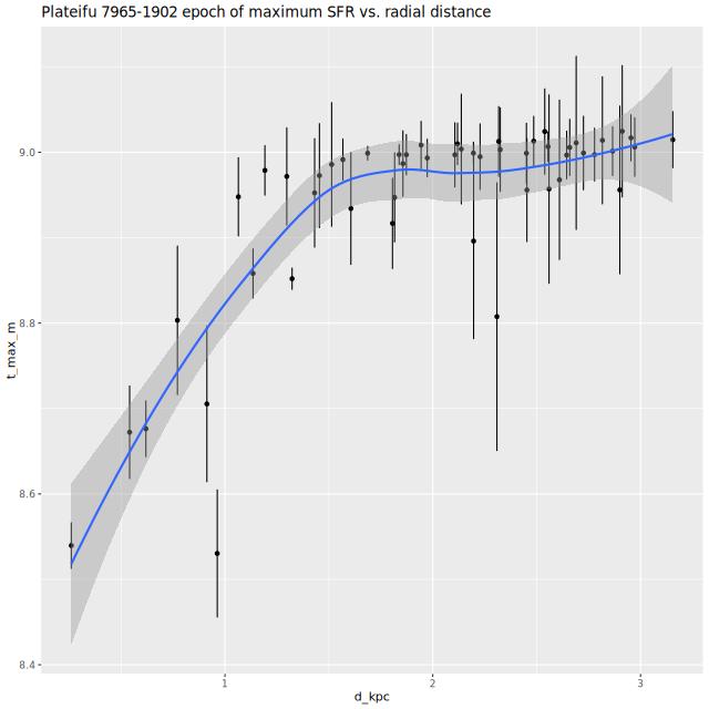
This plot should be compared to the upper right pane of Leung’s Figure 5. The agreement is rather good overall. I get a range of lookback times of ~1/3 – 1 Gyr, which is close to theirs, but with a steeper gradient in the center. In an earlier IFU based study Pracy et al. found a strong Balmer absorption index gradient in the inner ~1.5 kpc, consistent with my results.
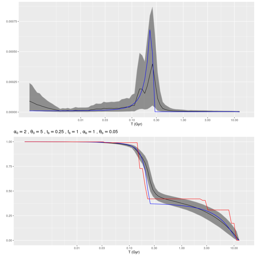
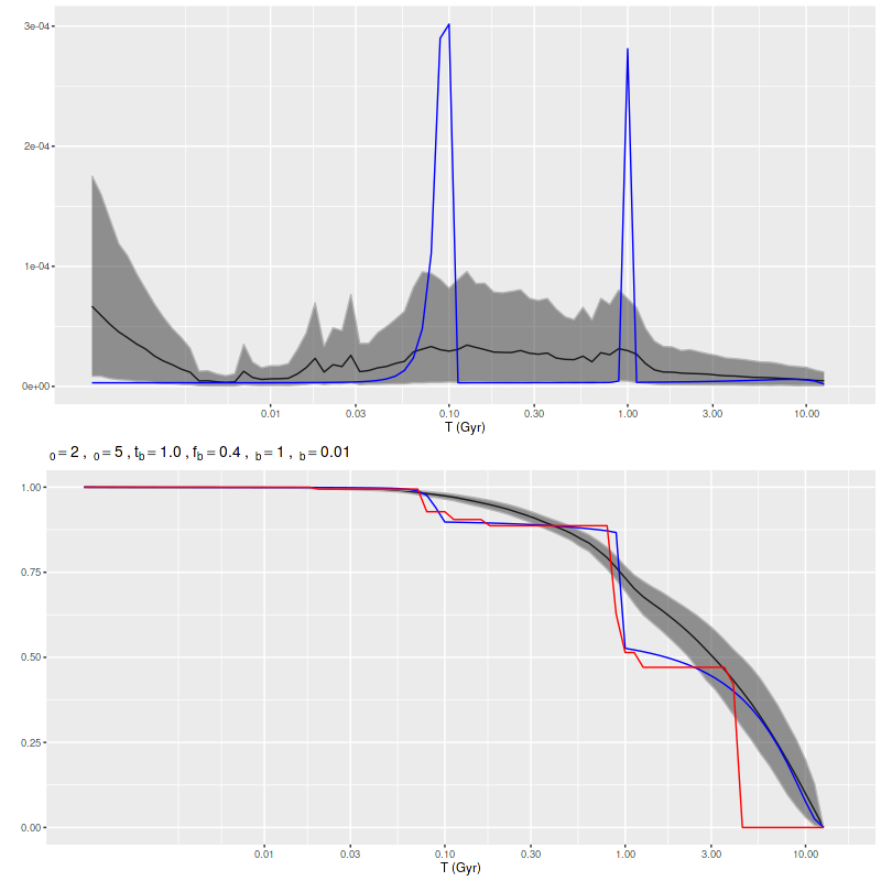
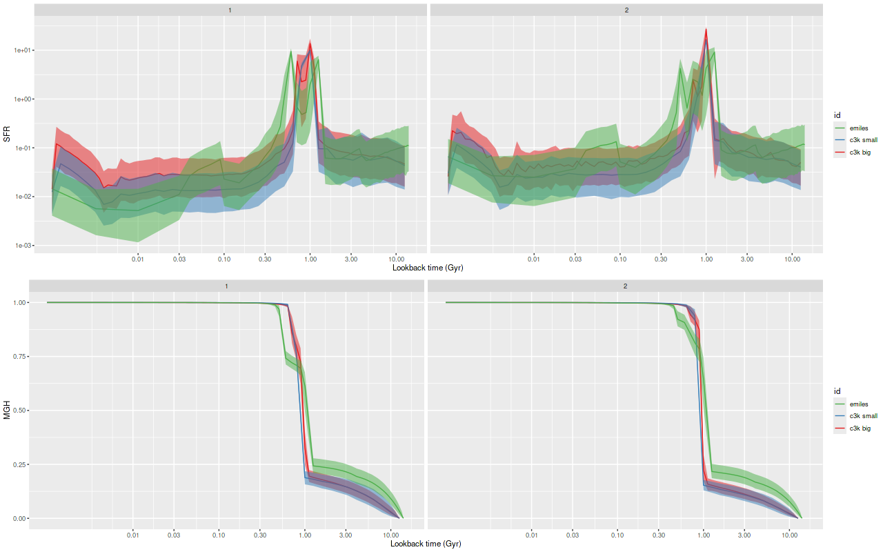
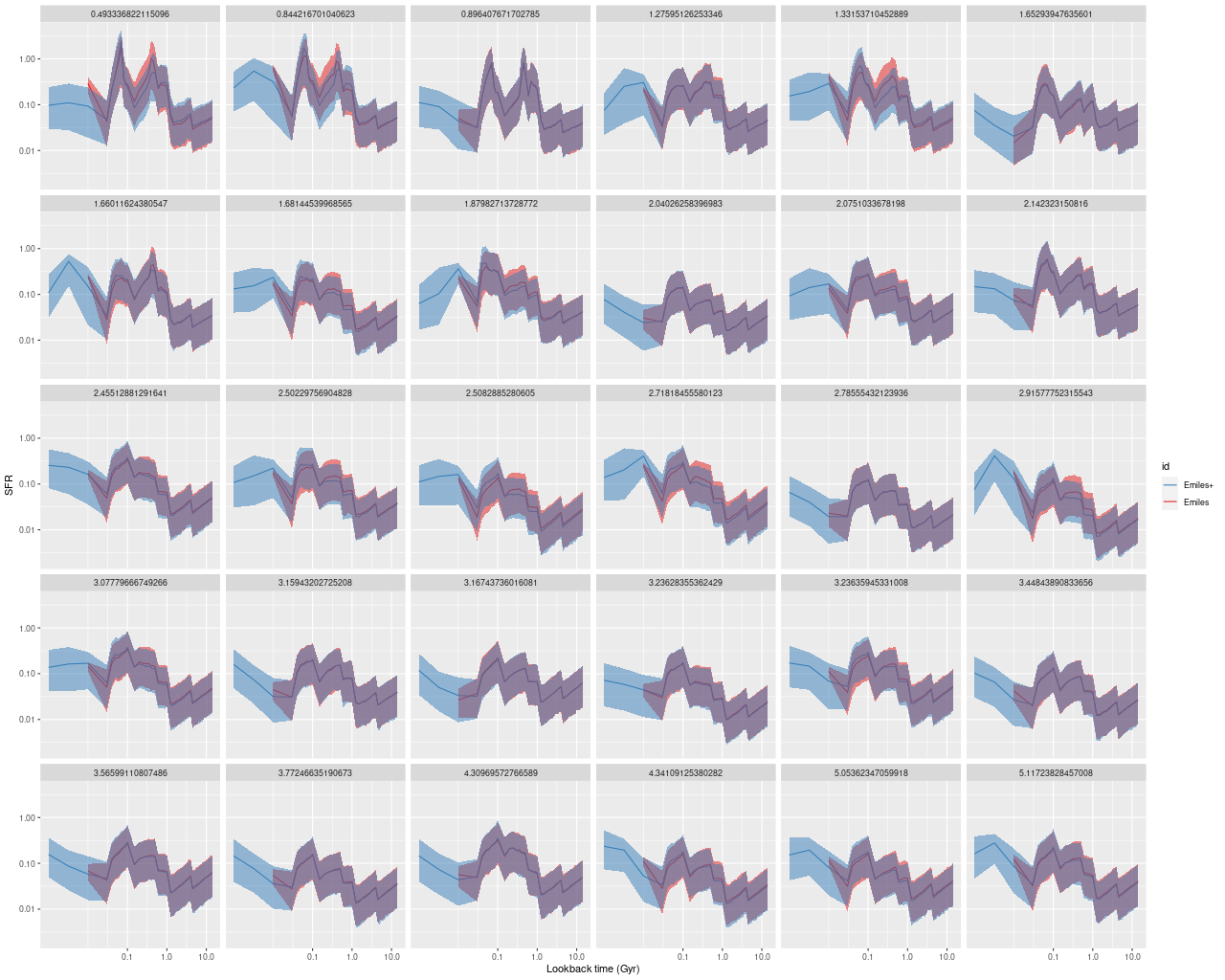
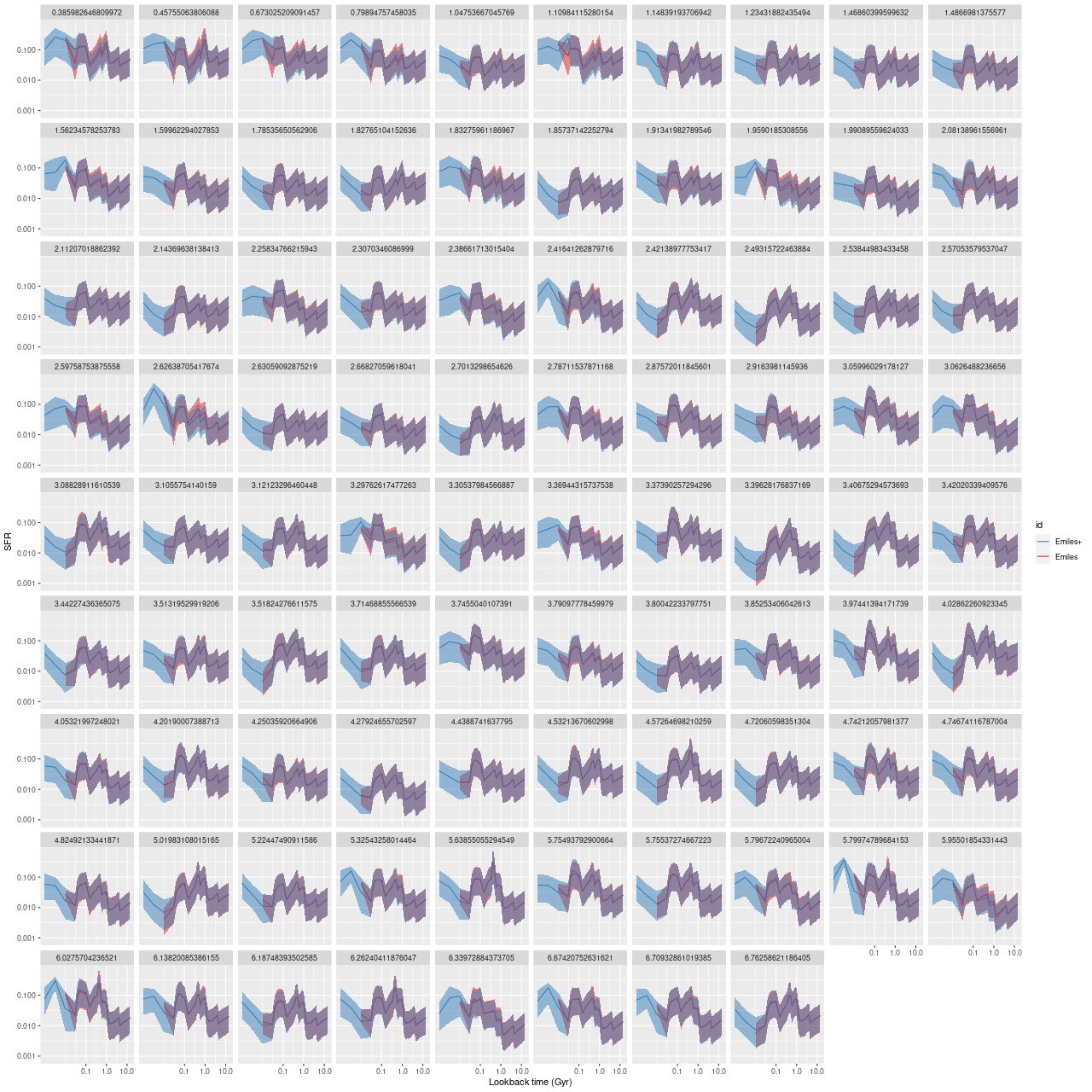
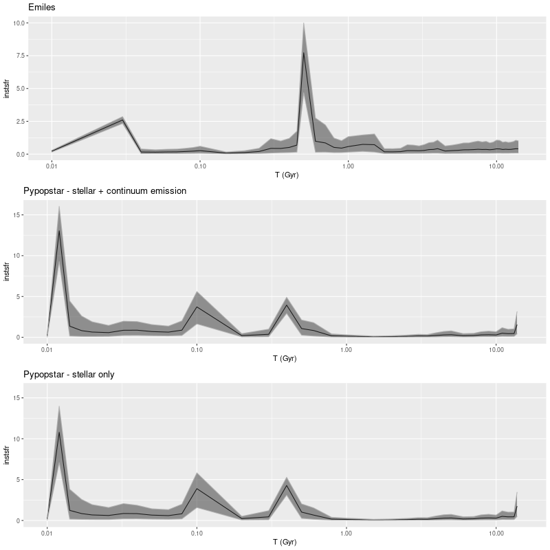
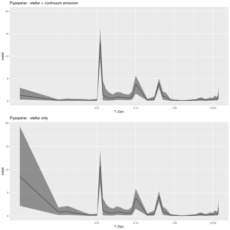
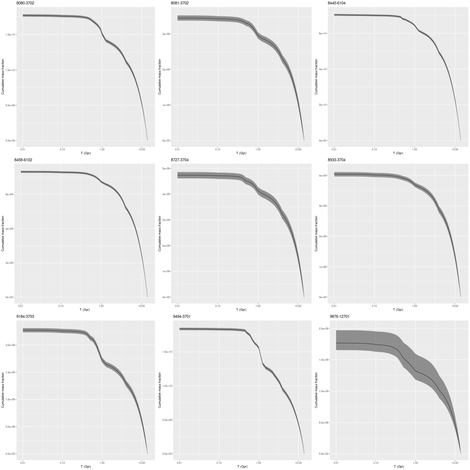
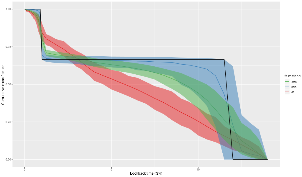
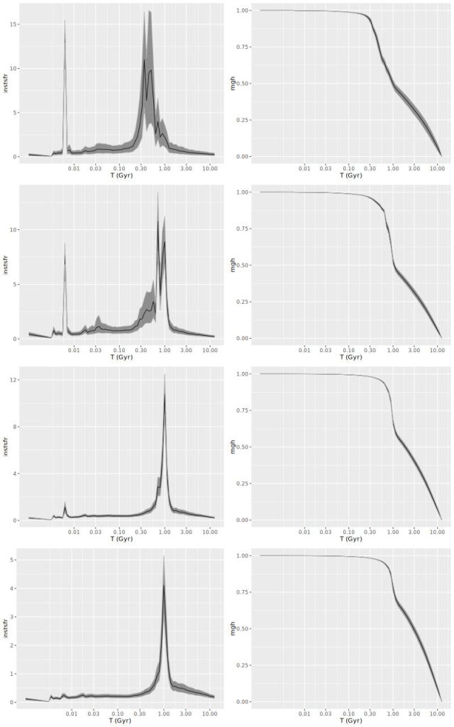
I’ll conclude with plots of model star formation histories, binned over circular annuli. These are shown as both star formation rate and present day mass growth histories. One striking feature of these plots is there appears to have been a recent revival of star formation within about 1reff of the nucleus. Whether this is real is hard to say, but note that the functional form adopted by Leung et al. cannot capture multiple bursts. This galaxy do. es have some ionized gas emission throughout, mostly with “Liner” like line ratios. This could be due in part to some ongoing star formation. In a few bins the very recent SFR exceeds the maximum in the earlier starburst, hence the decision to exclude the recent past in the maximum SFR calculation.
I’m still not sure how to estimate a burst mass fraction. An actual measurement would require a counterfactual estimate of the star formation history in the absence of whatever caused the burst, which we can’t really know. Perhaps a simple interpolation between the pre and post-burst star formation rates would be a reasonable guess if some objective definition of pre and post burst times could be devised. One thing I’ve noticed is mass growth histories of PSB regions usually go from mildly concave to convex for a period of time with a noticeable inflection point where the acceleration in star formation is a maximum. The total mass formed after that inflection point might be a useful proxy (but certainly an overestimate) for the burst fraction. In this case notice that inflection point shifts from ~1Gyr in the inner region to a little older farther out, while the total mass formed since then decreases from ~50% to ~30%. This suggests a negative gradient in burst strength, which is the opposite trend to that estimated by Leung et al.
One final comment about Leung et al.’s approach. As already noted they assume a functional form for the star formation rate, and specifically they assume an exponential decay model for the preburst evolution starting at some formation time. Although they never discuss this it’s clear from their graphs that the estimated formation times are strongly biased to the young side (see e.g. their Figure 8). For this galaxy for instance the estimated formation times range from just over 4Gyr ago to a little under 6Gyr. This corresponds to a redshift of formation of z≈0.5, which is well past “cosmic noon.” To the best of my knowledge there’s a general consensus that virtually(?) all present day galaxies began forming stars shortly after the Big Bang. While we can’t really say much about the truly ancient star formation histories of galaxies with recent star formation we can say with reasonable confidence that some took place. My non-parametric models always contain non-zero contributions at all ages, with at least plausible mass contributions from very old populations.
I will probably now turn to a more “birds’ eye” view of the entire Leung PSB sample. Since it’s been some time since I did the initial modeling I need to examine the model runs again. There were some with very poor data that need to be culled — these may or may not be the ones Leung excluded from analysis.
By my count there are ~6 obvious mergers in the RPSB sample and ~20 that are to varying degrees disturbed. These are in addition to NGC 2623, which recall was rejected as a candidate CPSB. I may take a separate look at the mergers.