
As I mentioned in the first post I’ve been doing star formation history (SFH) modeling by full spectrum fitting of galaxy spectra for several years. I’m going to quickly review what I do as a prelude to the next several posts where I plan to look at my proto-K+A galaxy in more detail. I’ll probably return to modeling details in the future. I still haven’t reached the point of having version controlled code let alone “publishing” it, but that’s not far off (I hope).
Full spectrum fitting is actually pretty simple, especially since other people have already done the hard work. The basic observational data is a set of monochromatic fluxes \(g_{\lambda}\) with estimated uncertainty at each point \(\lambda\) (\(\lambda\) is just a discrete valued index here) \(\sigma_{\lambda}\) or precision (inverse variance) \(p_{\lambda} = 1/\sigma^2_{\lambda}\) . For now let’s assume that observed fluxes are independently gaussian distributed with known variances (yes, this is a simplification).
The second main ingredient is a set of template spectra \(T_{\lambda, n}, n = 1, \ldots, N\), which nowadays usually comprises model spectra from a library of simple stellar population (SSP) models. If the physical parameters of the templates span those of the galaxy being modeled its spectrum would be fit with some nonnegative combination of the template spectra:
\(g_{\lambda} = \sum_{n=1}^N \beta_n T_{\lambda, n} + \epsilon_{\lambda}, ~~\beta_n \ge 0~~ \forall n\)
and by assumption the errors \(\epsilon_{\lambda}\) are gaussian distributed with mean 0 and standard deviation \(\sigma_{\lambda}\).
The spectroscopy we deal with is high enough resolution to be blurred by the constituents of the galaxy, so an additional ingredient is the “line of sight velocity distribution” (LOSVD), which must be convolved with the templates. Finally, it’s common to include additive or multiplicative functions to the model to allow for calibration variations or to model attenuation. I hopefully assume calibrations are well matched between observations and models and only attempt to model attenuation, usually with a Calzetti relation parametrized by optical depth. So, the full model looks like:
\(g_{\lambda} = \sum_{n=1}^N \beta_n (\mathcal{L}(v_n) \ast T_{\lambda, n}) \exp(-\tau_{V, n} A_{\lambda}) + \epsilon_{\lambda}, ~~\beta_n \ge 0~~ \forall n\)
where the \(v_n\) are (possibly vector valued) parameters of the LOSVD and \(\tau_{V,n}\) is the dust optical depth at V. These are nominally indexed by n to indicate that there may be different values for different model constituents. In practice I only consider a few distinct components.
An important insight of Cappellari and Ensellem (2004) that was dismissed in two sentences is that conditional on the parameters of the LOSVD and any multiplicative factors the subproblem of solving for the coefficients \(\beta_n\) is a linear model in the parameters with nonnegativity constraints, for which there is a fast, deterministic least squares algorithm due originally to Lawson and Hanson (1974). This greatly simplifies the nonlinear optimization problem because whatever algorithm is chosen for that only needs to optimize over the parameters of the LOSVD and optical depth. I currently use the general purpose optimization R package Rsolnp along with nnls for SED fitting. This is all similar to Cappellari’s ppxf but less versatile; my main interest is in star formation histories and I’ve found a better way to estimate them in a fully Bayesian framework. These days I mostly use the maximum likelihood fits as inputs to the Bayesian model implemented in Stan.
I have used several SSP libraries, but the workhorses recently have been subsets of the EMILES library with BaSTI isochrones and Kroupa IMF, supplemented with some unevolved models from BC03. One thing I do that’s not unprecedented but still somewhat unusual is to fit emission lines simultaneously with the stellar library fits. I do this by creating fake emission line spectra, one for each line being fit (usually the lower order Balmer lines and selected forbidden lines).
The models that I’m likely to discuss for the foreseeable future use separate single component gaussian fits to the stellar and emission line velocity distributions. I assume the velocity offsets calculated in the first step of the analysis are accurate, so the mean of the distributions is set to 0. I also use a single component dust model, usually with Calzetti attenuation relation. I don’t try to tie the relative strengths of emission lines, so attenuation is only directly modeled for the stellar component. These assumptions are obviously too simple for galaxies with broad emission line components or interacting galaxies with overlapping stellar components. For now I plan to ignore those.
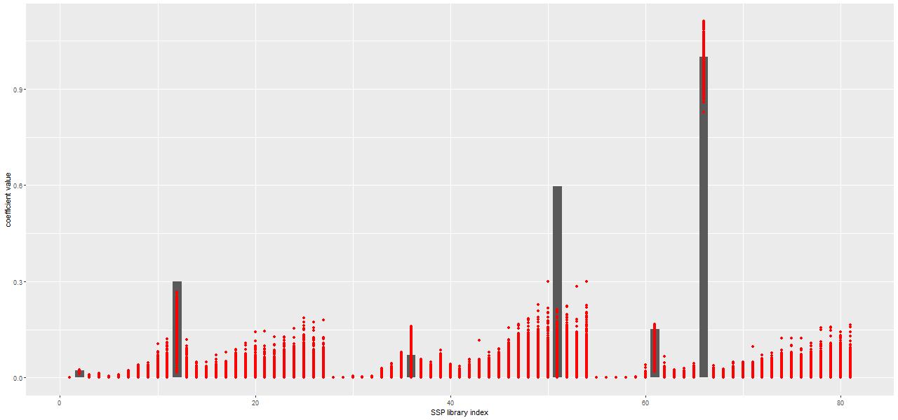
One interesting property of the NNLS algorithm for this application is that it always returns a parsimonious solution for the stellar component, with usually only a handful of contributors. An example of a solution from a fit to the central spectrum of the proto-K+A galaxy I introduced a few posts ago is shown below. The grey bars are the optimal contributions (proportional to the mass born in each age and metallicity bin) from the elements of the SSP library. This particular subset has 3 metallicity bins and 27 age bins ordered from low to high.
Only six (actually a seventh makes a negligible contribution) SSP model components are in the optimal fit, out of 81 in this particular library. Usually in statistics sparsity is considered a highly desirable property, especially in situations like this with a large number of explanatory variables. Considerable effort has been made to derive conditions where non-negative least squares, which has no tuning parameters, automatically produces sparse solutions (see for example Meinshausen 2013). However in this context sparsity is maybe not so desirable since we expect star formation to vary continuously over time in most cases rather than in a few short bursts as would be implied here: as a Bayesian my prior assigns positive probability density to star formation at all times.
But in the absence of a parametric functional form for star formation histories a fully Bayesian treatment of SED modeling is an extremely difficult problem. The main issue is that model spectra are highly correlated; if we could visualize the N dimensional likelihood landscape we’d see a long, curving, steep sided ridge near the maximum. I’ve tried a number of samplers over the years including various forms of Metropolis-Hastings and the astronomers’ favorite EMCEE and none of them are able to achieve usable acceptance rates. A few years ago I discovered that the version of “Hamiltonian Monte Carlo” (informally called the No U-Turn Sampler, or NUTS) implemented in the Stan modeling language is capable of converging to stationary distributions in a tractable amount of time. In the plot below the red dots indicate the range of values taken by each SSP model contribution in the post-warmup sample from a Stan run. Now all time and metallicity bins are represented in the model in amounts that are at least astrophysically plausible. For example instead of a single old component as in the NNLS fit the pre-burst history indicates continuous, slowly declining star formation, which is reasonable for the likely spiral progenitors.
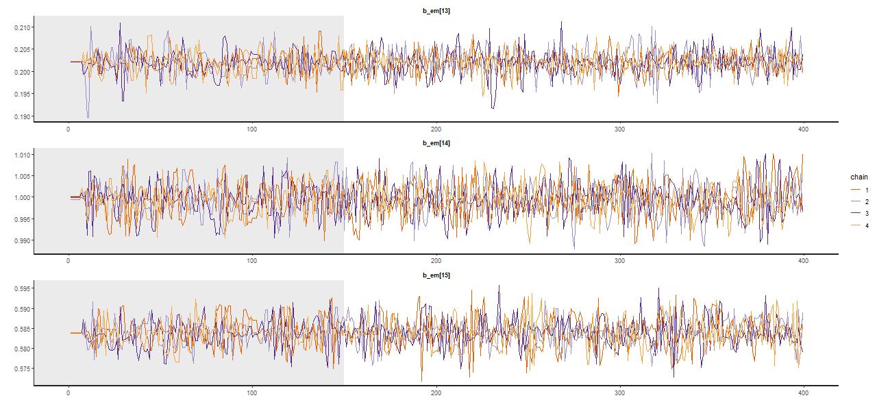
A trace plot, that is a sequential plot of each draw from the sampler, is shown for a few parameters below — these are the single old component in the maximum likelihood fit and the two in the surrounding age bins. Samples spread out rather quickly from the initialized values at the MLE, reaching in this case a stationary distribution about 2/3 of the way through the adaptation interval shown shaded in gray; I used a rather short warmup period of just 150 iterations for this run (the default is 1000, while I generally use 250 which seems adequate). There were 250 post warmup iterations for each of 4 chains in this run. No thinning is needed because the chains show very little autocorrelation, making the final sample size of 1000 adequate for inference. Most physical quantities related to the stellar contributions involve weighted sums of some or all coefficients, and these typically show little variation between runs.
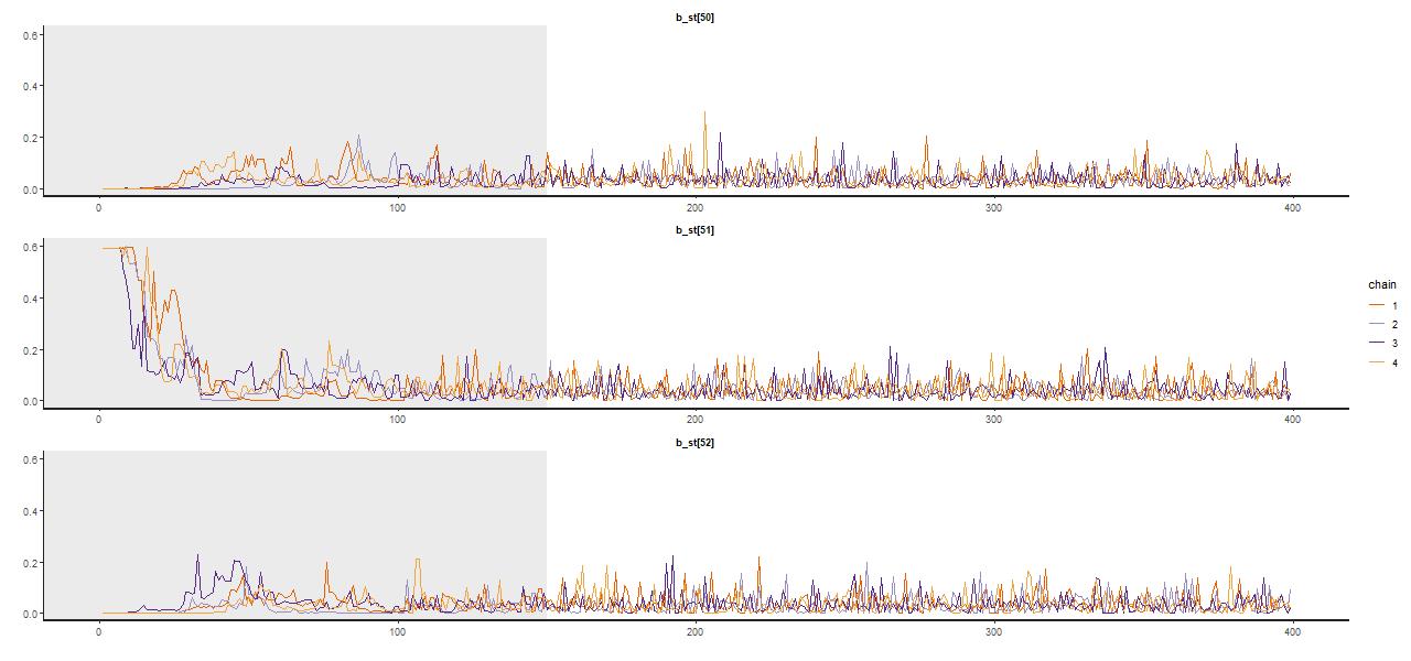
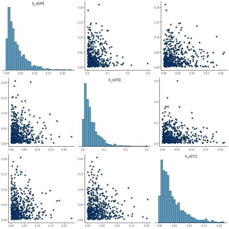
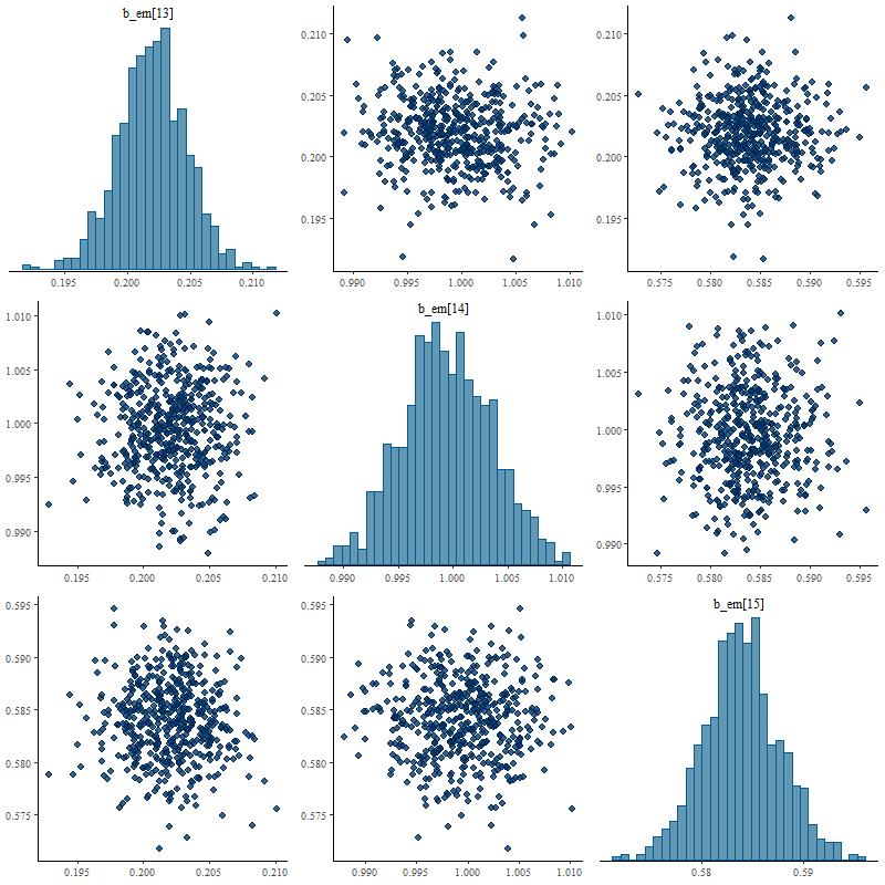
Posterior marginal distributions often have very long tails as shown here. This can be a problem for MCMC samplers and Stan is quite aggressive in warning about potential convergence issues. The quantities that I track tend to have much more symmetrical distributions.
Fits to emission lines tend to behave differently. If they’re actually present the MLE will have positive contributions (the coefficients are proportional to emission line fluxes). On the other hand in a passively evolving galaxy with no emission lines the MLE estimate is typically sparse, that is coefficient estimates will tend to be 0 rather than spuriously small positive values.
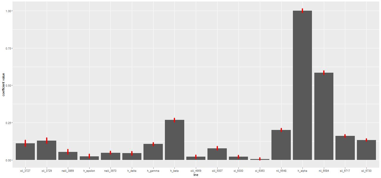
Sample values from Stan tend to stay centered on the ML fits (Hα and the surrounding [N II] lines are shown here):
Marginal posterior distributions tend to be symmetrical, close to Gaussian, and uncorrelated with anything else (except for the [O II] 3727-3729Å doublet, which will have negatively correlated contributions).
One thing that’s noteworthy that I haven’t discussed yet is that usually all available metallicity bins make contributions at all ages. I haven’t been able to convince myself that this says anything about the actual distribution of stellar metallicities, let alone chemical enrichment histories. In recent months I’ve started looking at strong emission line metallicity indicators. These appear to give more reliable estimates of present day gas phase abundances, at least when emission lines are actually present.