This post will be short. Eventually I’d like to add a reproducible real data example or two to the documentation of the software I just officially published. Even though I’m mostly working with MaNGA data these days it may not be practical to include an example since the smallest RSS file is ∼20MB and it can take days to fully process a single data set. The single fiber SDSS spectra on the other hand are only ~170-210KB in “lite” form. While I’m hunting around for suitable examples I’ll post a few results here. For today’s post a couple of randomly selected early type galaxies from my north galactic pole sample:
SDSS J121810.72+280230.4
SDSS J122140.20+222108.3
These don’t seem to be in any historical catalogs, so I’ll just call them by their SDSS designations of J121810.72+280230.4 and J122140.20+222108.3, or J1218+2802 and J1221+2221 for shorthand. The first appears to me to be a garden variety elliptical; the second might be an S0 — neither has a morphological classification listed in NED (a majority of GZ classifiers in both GZ1 and GZ2 called the second an elliptical). Galaxy 2 has a redshift of z=0.023, which puts it in or near the Coma cluster. Galaxy 1 is well in the background at z=0.081.
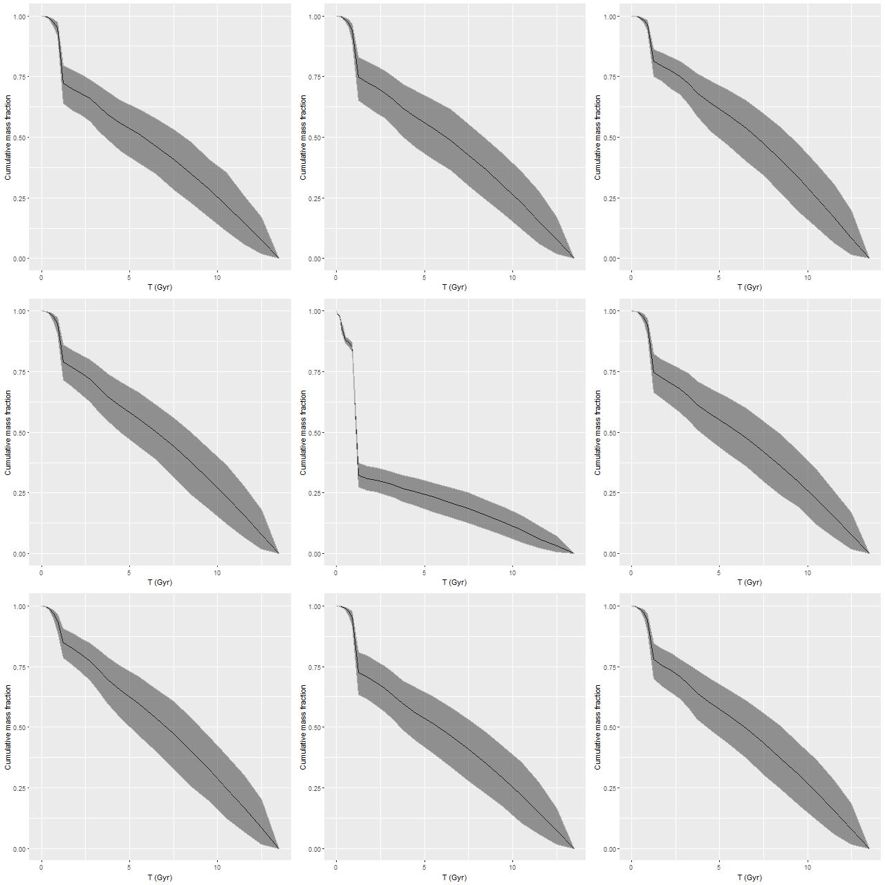
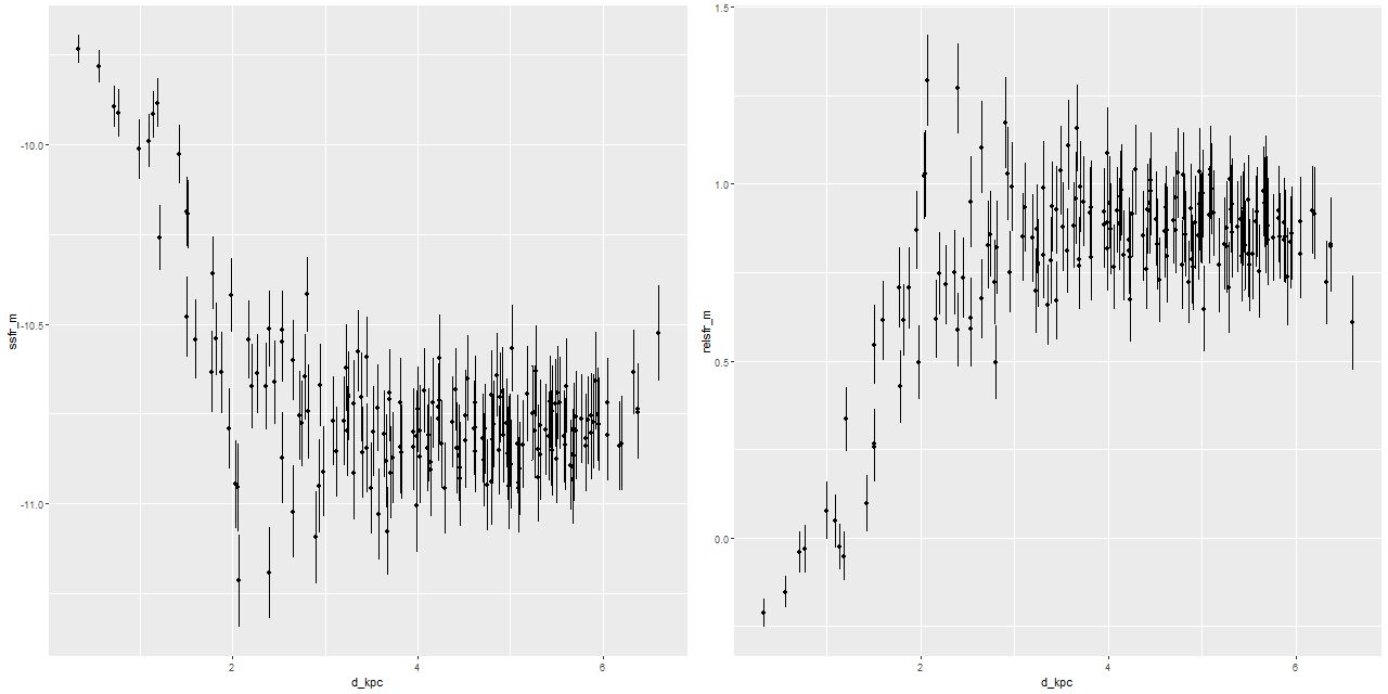
I modeled the star formation histories with my standard tools and the “full” EMILES ssp library (that is all 54 time bins in 4 metallicity bins). The Stan models both completed without warnings (one required some adjustment of control parameters). Here are some basic results. First, star formation histories, displayed as star formation rate against lookback time. I find it can be useful to use linear or logarithmic scales on either or both axes. Here I show SFR scaled both ways:
Star formation histories for 2 passively evolving galaxies
So-called non-parametric models for star formation histories are hoped for gold standards for SFH modeling, and here we see part of the reason: these have rather different estimated mass assembly histories despite similar looking spectra (see below or follow the links), and neither estimate is particularly close to commonly chosen functional forms.
There are some oddities to beware of however. For example literally 100% of the models I’ve run with any variation of the EMILES library show an uptick in mean star formation rate at 4Gyr, independent of the absolute estimated SFR. This can’t be real obviously enough, but I haven’t yet found an error or other specific reason for it. There may be other persistent zigs and zags in SFR at specific times, and these can vary with the SSP library. Overall I assign no particular significance to small variations in mean estimated star formation rates, especially at early times. I’m somewhat more inclined to take seriously late time variations (say, most recent Gyr), which may be wishful thinking.
The data aren’t inconsistent with a small amount of ongoing star formation (estimates of specific star formation rate averaged over 100Myr are shown — these have units of yr-1). SSFR’s in a range ~10-11 yr-1 are about an order of magnitude lower than an ordinary starforming galaxy in the local universe.
froPosterior distribution of specific star formation rate (100 Myr timescale)
Fits to the data are comparable, and satisfactory over most of the wavelength range of the spectra. A recent paper on arxiv (article id 1811.09799) mentioned some fitting issues with EMILES SSP libraries in the red. This can be seen here in the range ~6750-7500Å (rest frame). I don’t have an explanation either. It might be significant that the MILES stellar library spectra extend only to ~7300Å, with other data sources grafted on to the red extension, so there could be a calibration problem. On the other hand the prominent dip in this range is at least partly due to TiO absorption, so this could point to metal abundance variations not captured by EMILES.
Finally, I find it useful to model attenuation, even in ETGs that are often considered dust free. I just use a Calzetti attenuation curve in these models even though it was based on starburst galaxy SEDs and therefore may not be appropriate. This is a topic for possible future model refinement.
It took longer than I had hoped, but I finally have the R and Stan software that I use for star formation history modeling under version control and uploaded to github. There are 3 R packages, two of which are newly available:
spmutils: The actual code for maximum likelihood and Bayesian modeling of star formation histories. There are also tools for reading FITS files from SDSS single fiber spectra and from MaNGA, visualization, and analysis.
cosmo: A simple, lightweight cosmological distance calculator.
sfdmap: A medium resolution version of the all sky dust map of Schlegel, Finkbeiner and Davis (SFD) and a pair of functions for rapid access.
So far only cosmo is documented to minimal R standards. It’s also the most generally useful, at least if you need to calculate cosmological distances. sfdmap has skeleton help files; spmutils not even that. I plan to correct that, but probably not in the next several weeks.
The R packages are pure R code and can be installed directly from github using devtools:
The Stan files for SFH modeling that I’m currently working with are in spmutils/stan. I keep the Stan files in the directory ~/spmcode on my local machines, and that’s the default location in the functions that call them.
This code mushroomed over a period of several years without much in the way of design, so it’s not much use without some documentation of typical workflow. I will get around to that sometime soon (I hope).
In the last post I showed that the posterior distribution of the model parameters as estimated by Stan look rather different than the distribution of maximum likelihood estimates under repeated realizations of the noisy “observation” vector, but I didn’t really discuss why they look different. For starters it’s not because the Stan model failed to converge, nor is there any evidence for missed multimodality in the posterior. Although Stan threw some warnings for this model run they involved fewer than 1% of the post-warmup iterations and there was no sign of pathological behavior (by the way I recommend the package shinystan for a holistic look at Stan model outputs). Multimodality can happen — often it manifests as one or more chains converging to different distributions than the others, but sometimes Stan can fail to find extra modes. But I haven’t seen any evidence for this in repeated runs of this and similar models, nor for that matter in real data SFH modeling.I mentioned that I copied the prior over from my real data models and this is probably not quite what I wanted to use, and that gets us into the topic of investigating the effect of the prior in shaping the posterior. That’s not what caused the difference either, but I’ll look at it anyway.
The real reason I think is one that I still find paradoxical or at least sorta counterintuitive. The main task of computational Bayesian inference is to explore the “typical set” (a concept borrowed from information theory). There’s a nice case study by one of Stan’s principal developers showing through geometric arguments and some simple simulations that the typical set can be, and usually is, far (in the sense of Euclidean distance) from the most likely value and the distance increases with increasing dimensionality of the parameter space. We can show directly that is happening here.
Let’s first modify the model to adopt an improper uniform prior on the positive orthant, which just requires removing a line from the model block of the Stan code (if no prior is specified it is implicitly made uniform, which in this case is improper):
parameters {
  vector<lower=0.>[M] beta;
}
model {
  y ~ normal(X * beta, sdev);
}
Modern Bayesians usually recommend against the use of improper priors, but since the likelihood in this model is Gaussian the posterior is proper. The virtue of this model is the maximum a posteriori (MAP) solution is also the maximum likelihood solution. Stan can do general nonlinear optimization as well as sampling, using by the way conventional gradient based algorithms rather than Monte Carlo optimization.
First, I run the sampler on this model, and extract the posterior:
I do this to get a starting guess for the optimizer and because we’ll do some comparisons later. For some reason rstan’s optimization function requires as input a stanmodel object rather than a file name, so we call stan_model() to get one. Then I call the optimizer, adjusting a few parameters to try to get to a better solution than with defaults:
Now let’s use these to initialize the chains for another Stan model run (I also adjusted some of the control parameters to get rid of warnings from the first run):
Now examine trace plots for the first few warmup draws for a few parameters. The top rows trace the first 100 warmup iterations. The right 4 are initialized with the approximate maximum likelihood solution, the left are from the first randomly initialized run. The ML initialized chains quickly move away from that point and reach stationary, well mixed distributions in just a few iterations. The randomly initialized chains take slightly longer to get to the same stationary distributions.
Stan runs with improper uniform prior – sample traceplots (TL) warmup iterations with random inits (TR) warmup iterations with nnls solution inits (BL) post-warmup with random inits (BR) post-warmup with nnls solution inits
And the resulting interval plot for the model coefficients isn’t noticeably different from the first run:
Coefficient posteriors with improper uniform prior
Nowadays Bayesians generally advise using proper priors that reflect available domain knowledge. I had done that originally but without thinking that the prior wasn’t quite right given the data manipulations that I had performed. A better prior that incorporates “domain” knowledge without being too specific might be something like a truncated normal with the same scale parameter for each coefficient, which in this case can reasonably be set to 1. That’s accomplished by adding back just one line to the model block:
model {
  beta ~ normal(0, 1.);
  y ~ normal(X * beta, sdev);
}
which leads to the following posterior interval plot compared to the original:
(L) N(0, 1) prior (R) original variable width prior
See the difference? Close inspection will show some minor ones, but it’s not immediately clear if they’re larger than expected from sampling variations.
Can we induce sparsity?
Here are a couple ideas I thought might work but didn’t. One way to induce sparsity in regression models is called the lasso, or more technically L-1 penalized regression. This is just least squares with an added penalty proportional to the absolute values of the model parameters. A more or less equivalent idea in Bayesian statistics is to add a double exponential or Laplacian prior. Since the parameters here are non-negative we can use an exponential prior instead.
Yet another possible prior inspired by “domain knowledge” is to notice that the coefficient values I picked sum to 1. A sum to 1 constraint can be programmed in Stan by declaring the parameter vector to be a simplex. Leaving out an explicit prior will give the parameters implicitly uniform priors.
parameters {
  simplex[M] beta;
}
model {
  y ~ normal(X * beta, sdev);
}
Interestingly enough for possible future reference this model ran much faster than the others and threw no warnings, but it didn’t produce a sparse solution:
More posterior interval plots (L) exponential prior (R) unit simplex parameter vector
Back to the drawing board and with a bit of web research it turns out there is a fairly standard sparsity inducing prior known as the “horseshoe” described in yet another Stan case study by another principal developer, Michael Betancourt. The parameter and model block for this looks like
parameters {
  vector<lower=0.>[M] beta;
  real<lower=0.> tau;
  vector<lower=0.>[M] lambda;
}
model {
  tau ~ cauchy(0, 0.05);
  lambda ~ cauchy(0, 1.);
  beta ~ normal(0, tau*lambda);
  y ~ normal(X * beta, sdev);
}
This is the “classical” horseshoe rather than the preferred prior that Betancourt refers to as the “Finnish horseshoe.” This took some fiddling with hyperparameter values to produce something sensible that appeared to converge, but it did indeed produce a sparse posterior:
Posterior intervals – Horseshoe prior
This run did find two posterior modes, and this illustrates the typical Stan behavior I mentioned at the beginning of this post. Two chains found a mode where beta[49] is large and beta[51] near 0, and two found one with the values reversed. There’s no jumping between modes within a chain:
A bimodal posterior
Finally, here are the distributions of log-likelihood for the 6 priors considered in the last two posts:
Posterior distributions of log-likelihood for 6 priors
Should we care about sparsity? In statistics and machine learning sparsity is usually considered a virtue because one often has a great many potential predictors, only a few of which are thought to have any real predictive value. In star formation history modeling on the other hand astronomers usually think of star formation as varying relatively smoothly over time, at least when averaged over galactic scales. Star formation occurring in a few discrete bursts widely separated over cosmic history seems unphysical, which makes interpreting (or for that matter believing) the results challenging.
One takeaway from this exercise is that in a data rich environment the details of the prior don’t matter too much provided it’s reasonable, which in the context of star formation history modeling specifically excludes one that induces sparsity — despite the fact that in this contrived example the sparsity inducing prior recovers the inputs accurately while generic priors do not. Of course maximum likelihood estimation does even better at recovering the inputs with far less computational expense.
There was a bit of controversy that played out earlier this year on arxiv and the pages of MNRAS on a subject of interest to me, namely full spectrum modeling of (simulated) galaxy SEDs. It began with a paper by Ge et al. (arxiv article ID 1805.03972) comparing outputs of STARLIGHT and pPXF, two popular full spectrum fitting codes, on very simple one and two component synthetic spectra with varying ages, reddening, and S/N. They found significant biases in mass to light ratios and other derived quantities in STARLIGHT output in some cases — primarily ones with a young population and large reddening — that oddly got worse with increasing S/N, while pPXF generally had smaller biases that improved with increasing S/N. They also obtained poor fits to the data in the cases with the most biased outputs, and noted multiple order of magnitude differences in execution time.
Not surprisingly this was soon followed with a heated rebuttal by cid Fernandes, the primary author and maintainer of STARLIGHT. This was first posted on arxiv with the title “Rebutting fake news on full spectral fitting” (article ID 1807.10423). The published version with the more temperate title “On tests of full spectral fitting algorithms” appeared in the November 2018 MNRAS (and is apparently not paywalled, although Ge et al. is).
As I read it there were three main threads to the rebuttal:
A single, “hitherto deemed unimportant” line of code was responsible for the poor performance at large input reddening values. The offending line apparently limits the initialization of reddening values to what would normally be reasonable for realistic galaxy spectra.
But, even without modifying the code good results could have been achieved by modifying configuration files.
And anyway the worst performance was for an unrealistic edge case that wouldn’t be encountered in real work.
The one problem I have with this is that STARLIGHT is not open source at present, and without the source code the otherwise trivial issue isn’t easily discoverable, let alone fixable. As for the other points it should have been fairly obvious that getting poor results when the ingredients used to fit a data set are exactly the ones used to generate the data is a sure sign of convergence failure.
Actually though this post isn’t about these papers or directly about these two codes. It wasn’t clear to me why Ge et al. wrote the paper they did or why editors and referees considered it publishable in MNRAS — while fake data exercises are a necessary part of software validation there wasn’t any larger scientific purpose to their work. But I did like the idea of looking at an unrealistic edge case for reasons that I hope will become obvious. What I’m going to examine is even simpler: I construct a mock spectrum as a linear combination of two SSP model spectra from the EMILES library, perturb it with random noise, and fit it with a subset of EMILES using three different fitting methods. Neither convolution with a line of sight velocity distribution nor reddening is done, and these aren’t modeled in the fits. The fitting methods I use are
non-negative least squares using the R package nnls, which implements Lawson & Hanson’s 1974 algorithm. This is a crucial part of both my code for maximum likelihood estimation of star formation histories and pPXF, which uses the implementation (probably based on the same FORTRAN code) in scipy.optimize.
A Stan model that’s a simplified version of the one I use for Bayesian SFH modeling.
STARLIGHT uses a Monte Carlo based optimization scheme, and I thought it would be interesting to compare the methods I use regularly to a state of the art approach to Monte Carlo optimization. To that end I chose the “differential evolution” algorithm implemented in the package RcppDEoptim. I should emphasize at the outset that this is a very different algorithm than the one in STARLIGHT and none of the results I present here have any direct relevance to it.
I didn’t think it was worth the effort to version control this or create a Github project, but I did upload all code and data needed to reproduce the graphics in this post to my dropbox account. I don’t necessarily recommend running this because it’s quite time consuming, but if you want to try it just download the entire folder and after starting R set the working directory to toynn and type source("toynnscript.r", echo=TRUE). Then go away and come back in 12 hours or so.
Let’s look at the script. The first few lines load the libraries I need and set some options for rstan:
## libraries we'll need

require(rstan)
require(nnls)
require(RcppDE)
require(ggplot2)
require(bayesplot)
require(gridExtra)
source("toynnutils.r")

## set a few options

ncores <- min(parallel::detectCores(), 4)
options(mc.cores = ncores)
rstan_options(auto_write = TRUE)
set.seed(654321L)
Stan can run multiple chains in parallel on any multi-core architecture and defaults to 4 chains, so the line that starts with ncores <- will be used to tell Stan to use the smaller of the number of cores detected or 4. I set and reset the random number seed several times in this script for exact reproducibility. Next I set up the fake data:
## load emiles ssp library and extract parts we need

load("emiles.sub1.rda")
X <- as.matrix(emiles.sub1[, 110:163])
X <- scale(X, center=FALSE)
mstar <- mstar.emiles[109:162]
ages <- ages.emiles
lambda <- emiles.sub1[,1]
rm(emiles.sub1, mstar.emiles, ages.emiles, Z.emiles, gri.emiles)

nr <- nrow(X)
nv <- ncol(X)

beta_act <- numeric(nv)
beta_act[22] <- 0.3
beta_act[50] <- 1 - beta_act[22]
sdev <- 0.02
y_act <- as.vector(X %*% beta_act)
y <- y_act + rnorm(nr, sd=sdev)
dT <- diff(c(0, 10^(ages-9)))
stan_dat <- list(N=nr, M=nv, X=X, y=y, dT=dT, sdev=sdev)
The subset of the EMILES library provided here has 4 metallicity bins and 6000 wavelength points between about 3465 and 8864Å. I extract the solar metallicity model spectra, and although it’s overkill for this exercise I retain all 6000 wavelength points. The two nonzero components are 1 and 12Gyr old SSPs. I add IID gaussian random noise to the model spectrum with a standard deviation that will be treated as known. Real modern spectroscopic data always comes with an error estimate for each flux measurement, and these are typically treated as accurate in SED modeling.
The script runs the Stan model next, so let’s look at the Stan code:
There are just two lines in the model block: one to specify a prior and one for the likelihood. The prior was copied directly from my “real” Stan model for SFH modeling. It sets the scale parameter to be proportional to the width of the age bin each SSP model covers, and since the parameter values are proportional to the mass born in each age bin this will make a typical draw from the prior have a roughly constant star formation rate over cosmic history. Unfortunately I rescale the data in a different way for this exercise and the prior is doing something different, but no matter for now. Continuing with the script:
## in the stan call set open_progress to FALSE if using rstudio
## max_treedepth = 13 should make convergence warnings go away
## this will take a while...

system.time(stanfit <- stan(file="simplenn.stan", data=stan_dat, chains=4, iter=1000, warmup=500,
              seed=54321L, cores=ncores,
              open_progress=TRUE, control=list(max_treedepth=13)))
I set the number of warmup and total iterations to half the rstan defaults, which is plenty. Stan gets to stationary distributions for all parameters remarkably quickly. In the comments I optimistically guess that all convergence warnings will go away. Actually there was a warning that “17 transitions exceeded (sic) the maximum treedepth.” In this case the warnings don’t actually point to any convergence issues. BTW this took about 1 1/4 hours on a 2018 vintage PC built around Intel’s second most powerful consumer CPU as of late 2017.
In the paper that introduced pPXFCappellari and Ensellem (2004) had the important insight that non-negative least squares produces the maximum likelihood estimator for the stellar contributions in SED fitting (in astronomers’ parlance it minimizes χ2). Solving NNLS problems is important in a number of disciplines and many algorithms exist, several of which are implemented in various R packages. It turns out though that an old one published by Lawson and Hanson works pretty well for the type of data used in SED modeling. A remarkable feature of NNLS is that it tends to return sparse (or parsimonious as I put it in an earlier post) parameter estimates. In fact with real data I find that it always returns sparse solutions for the stellar components. Getting back to the script the last major computational efforts involve repeated calls to nnls and a smaller number of simulations using DEoptim (which is much slower):
## simulate lots of nnls fits

system.time(nnfits <- sim_nn(X, y_act, sdev=sdev, N=2000))

## nnls likes to produce sparse solutions, but not so sparse as the input in this case
qplot(nnfits$simdat$nnzero,geom='histogram',binwidth=1) +
      geom_vline(xintercept=median(nnfits$simdat$nnzero)) +
      xlab("# components")+ggtitle("# components in NNLS fits")
table(nnfits$simdat$nnzero)

## simulate not so many calls to DEoptim. This also takes a while...

system.time(defits <- sim_de(X, y_act, sdev=sdev, N=100))

x11()
qplot(defits$simdat$deltall,geom='histogram',bins=10) +
    xlab(expression(paste(delta~"log likelihood"))) +
    ggtitle("fractional difference in log likelihood between DE fit and NNLS")
The function sim_nn is in the file toynnutils.r. This just generates N randomly perturbed sets of the observation vector y, fits them using nnls, and returns some information about the fits (in Windows the CPU time estimates will be not very accurate):
sim_nn <- function(X, y_act, sdev=0.02, N=1000, seed=12345L) {
  require(nnls)

  set.seed(seed)
  nnzero <- numeric(N)
  ctime <- numeric(N)
  ll <- numeric(N)
  nr <- length(y_act)
  nv <- ncol(X)
  B <- matrix(0, N, nv)
  res <- matrix(0, N, nr)
  for (i in 1:N) {
    y <- y_act + rnorm(nr, sd=sdev)
    ctime[i] <- system.time(nnsol <- nnls(X,y))[1]
    B[i,] <- nnsol$x
    nnzero[i] <- nnsol$nsetp
    ll[i] <- sum(dnorm(residuals(nnsol), sd=sdev, log=TRUE))
    res[i, ] <- residuals(nnsol)/sdev
  }
  list(simdat=data.frame(ctime=ctime, nnzero=nnzero, ll=ll), B_nn=B, res_nn=res)
}
The first ggplot2 call in the script produces this histogram of the number of non-negative components of the nnls fits. As expected and consistent with typical real data nnls always returns sparse fits, although almost never quite so sparse as the input. The call to table() returns
Number of nonzero parameter estimates in NNLS fits
Perhaps the most interesting result of these simulations are the distributions of parameter estimates — these show 50 (thick lines) and 90% (thin lines) intervals, with median values marked by symbols:
Parameter estimates from different fitting methods: (L) posterior distribution from Stan (M) NNLS (R) DEoptim
What’s most striking to me at least is how different the posterior marginal distributions from Stan (left panel) are from the maximum likelihood fits (middle). Star formation is much more extended in time in the Stan model, with both “bursts” replaced with broad ramps up and decays. The Monte Carlo optimization results look superficially similar to the Stan posterior, but as I’ll show soon there are different causes for their behavior.
Let’s take a closer look at the distributions of some of the parameter values. This is called a pairs, or sometimes corner, plot — it displays the marginal distribution of each selected parameter along the diagonal and fills out the remaining rows and columns with the joint distributions of pairs of parameters. For this plot I just selected the two non-zero inputs and the surrounding age bins. The top rows are the Stan posterior, the bottom the nnls fits from the 2000 sample simulation.
Pairs plot for selected parameters: (T) Posterior draws from Stan model (B) NNLS estimates
In frequentist statistics a confidence interval is a statement about the behavior of the estimator for a parameter under repeated experiments with the same conditions. It’s not a statement about the parameter itself, which is forever unknowable. A Bayesian confidence interval (to the fussy, credible interval) on the other hand is a statement about the parameter itself.
I’m unaware of any formula for confidence intervals of nnls coefficient estimates, but the simulation we performed gives good numerical estimates of the distribution of parameter values, and these are clearly significantly different from the posterior distributions from Stan. So, not only is there a difference in interpretation between frequentist and Bayesian confidence intervals in this case the values obtained are significantly different as well.
Mass growth histories have become a popular tool for visualizing SFH models, so for fun I created mock histories for the three methods tested here. These show medians and 95% confidence bands. The input MGH just falls within the 95% confidence band of the nnls fits, although the median has more extended mass growth.
Model “mass growth histories” from simple two component input
Turning next to fits to the data let’s look first at the overall fits measured by summed log-likelihood. Remember that the nnls solution is the maximum likelihood estimator and therefore neither of the other fitting methods can exceed its log-likelihood for any given realization of the data.
Here’s the posterior log-likelihood from the Stan model run. The vertical line to the right is for the nnls fit. The Stan fit average falls short of the maximum likelihood by about 0.1%. We’ll examine why in more detail next post.
log likelihood of posterior fits
I only ran 100 simulations of the “differential evolution” optimizer because it takes rather a long time (average ~450 sec. per data realization on my PC). The output log-likelihood consistently falls about 1% short of the nnls solution:
fractional δ log likelihood between DEoptim and NNLS fits for 100 data realizations
This shows the progress of the optimizer for a single data realization. Progress is rapid at first, but it slows down as it gets close to the optimum and can stall out for many iterations. This algorithm has a hard time getting to a sparse solution.
Progress of DEoptim fits (difference in log likelihood with NNLS fit)
Next let’s look at detailed fits to the data. The top pane shows the unperturbed spectrum (black points) and a 95% confidence band for the posterior predictive fit (green ribbon) from the Stan model. What’s that? Simple: take parameter draws from the posterior and generate new data according to the model. This is done with the following lines in the generated quantities block of the Stan code:
It turns out that the 95% confidence band covers 100% of the true, unperturbed, spectral values and 95% of the perturbed ones, which indicates a successful model.
The remaining panes show several sets of normalized residuals. The first surprised me a bit at first: this shows the residuals (observed – model) of the Stan model posterior. The “points” in this plot are actually error bars — it turns out the range of residuals at any wavelength is rather small (I naively expected that residuals at each point would vary randomly around 0). The residuals from the posterior predictive fits shown in the next panel do show this behavior. This and the remaining panels display median values as points and 95% confidence bands.
The 4th pane shows the errors in the posterior predictive fits, that is the original unperturbed data minus the posterior predictive values. There are hints of systematics here: a bit of curvature at the red and blue ends of the spectrum and a few absorption lines are slightly misfit.
The final two are residuals from the simulated nnls and Monte Carlo optimization fits. The nnls fits have exactly the expected statistical behavior while the latter clearly struggles to fit the data. This is because the overly extended star formation histories reached in the number of iterations allotted result in stellar temperature distributions that aren’t quite right, affecting both the continuum and many absorption features.
Fits to data: T) input spectrum and posterior predictive fit from Stan model 2) Residuals from Stan model posterior 3) Residuals from posterior predictive fits 4) Errors from posterior predictive fits 5) Residuals from NNLS fits 6) Residuals from DEoptim fits
Finally, here is a comparison of the distribution of the residuals in the Stan fit to the same data realization fit by nnls, the colored bands being the former. These show kernel smoothed density estimates on the left and empirical CDF on the right.
Comparison of distribution of residuals in Stan model fit with nnls fit
It’s sometimes suggested in the SFH modeling literature to get parameter uncertainty estimates by randomly perturbing data and refitting it. This is a computationally viable strategy with a competent non-negative least squares solver, but as we saw above this is likely to produce very different estimates than a proper Bayesian analysis.
A paper showed up on arxiv in early August titled “An early-type galaxy with an inner star-forming disk” by Li et al. (article id 1808.01730) that describes a system observed by MaNGA that’s rather similar to the one I have been writing about in recent posts, namely an apparent post-merger ETG with ongoing star formation. The paper is a little light on details, but it’s refreshingly short and not technically demanding. Unfortunately their discovery claim is incorrect: this galaxy was identified as a star forming elliptical in Helmboldt (2007), who also measured its HI mass to be 5.4±0.5 × \(10^8 \mathsf{M}_{\odot}\), about 5% of its baryonic mass.
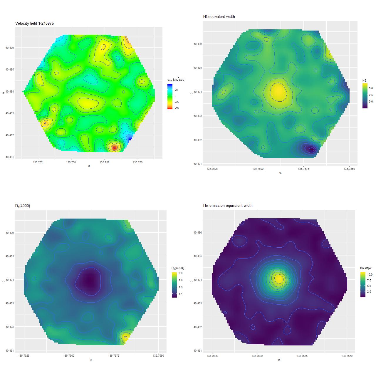
Of course I did my own analysis which I’ll summarize in this post, also filling in some details missing from the paper. The first step in my analysis is to compute a velocity field (actually what I compute are redshift offsets, but these are easily converted to line of sight velocities). One of the first things I noticed is that while this is qualitatively similar to the one published by Li et al. (and shown twice!), the rotating inner component has nearly 3 times the maximum rotation velocity as their stellar velocity map.
Velocity field estimated from RSS data
So, naturally concerned that there was an error in my processing of the RSS data I downloaded the data cube and ran my code on that, getting the velocity field shown below on the left, which is evidently nearly identical.
Recall that my redshift offset measurement routine does template matching very similar to the SDSS spectro pipeline, using for templates a set of eigenspectra from a principal components analysis of a largish set of SDSS single fiber spectra from a high galactic latitude sample. These naturally encode information about both emission and absorption lines, with the code returning a single blended estimate. This works fine when ionized gas and stars are kinematically tightly coupled, but not so well when they’re not. Suspecting that emission lines were dominating the velocity estimates in the inner regions, as something of a one-off experiment I masked the area around emission lines in the galaxy spectra and reran the routine, getting the velocity field on the right.
Now this agrees in some detail with the stellar velocity field published by Li et al. (visual differences are mostly due to different color palettes). So an interesting first result is that not only is there a rotating, kinematically decoupled core but the stars and ionized gas within the core are decoupled from each other. This would seem to point to a recent injection of fresh cold gas.
Unfortunately they only published the stellar velocity field even though the official data analysis pipeline calculates separate ones for stars and gas, so I won’t be able to verify this result until value added kinematic data is made available.
(L) Velocity field estimated for data cube
(R) Stellar velocity field
For reference here is the spectrum from the central fiber. Wavelengths are vacuum rest frame and fluxes are corrected for foreground galactic extinction.
Central fiber spectrum, plateifu 8335-6101
As with the previous galaxy I did two sets of star formation history models. The first set a low S/N threshold for binning spectra and used an 81 SSP model subset of EMILES for fitting. For the second run I bin to a considerably higher target S/N and fit with the larger 216 SSP model set with the full BaSTI time resolution. The second data set has 25 coadded spectra with mean S/N per pixel ranging from 18-60.
For a quick comparison of the two sets of runs here are model mass growth histories summed over all spectra. Both indicate that a very substantial burst of star formation occurred beginning ~1.25Gyr ago (curiously, this is the same time as the initial burst in the galaxy KUG 0859+406 that I previously wrote about — part 1, part 2, part3). The present day stellar mass is just under \(1 times 10^{10} mathsf{M}_{odot}\), in agreement with the value cited by Li et al.
Summed model mass growth histories, emiles subset and “full” emiles
I find that ongoing star formation is largely confined to the KDC, in agreement with Li et al., so after running the models for the 25 bins I partitioned them into a core set and an outer set, with the core set comprising the bins within about 4×2″ (1.5 x 0.75 kpc semi-major and semi-minor axes) of the nucleus as shown below.
Stellar mass density for binned data, showing outlines of bins and core region
The summed star formation history models are shown below. As with my previous subject there was a galaxy wide burst of star formation ~1Gyr ago, but unlike it star formation declined monotonically after that, with no more recent secondary burst. The ongoing star formation in the central region is seen to be a relatively recent (last ~100Myr) uptick. This leads me to a slightly different interpretation of the data — the authors suggest that we are seeing the late stages of a gas rich major merger. I would say rather that the merger was completed ~1Gyr ago and that gas has recently been recaptured. This is consistent with simulations that show in the absence of AGN feedback star formation can proceed for some time after a merger. It’s also consistent with the observed reservoir of neutral hydrogen, which is sufficient to fuel star formation at the current level for another ~1Gyr.
(L) Model Star formation history, inner core
(R) Star formation history, outside core
Here are some additional results of the analysis of the 25 binned spectra. All of these agree with Li et al. where comparable results are displayed.
First, the Hδ absorption line index vs. 4000Å break strength index Dn(4000):
Lick HδA vs. Dn(4000)
Contour lines are my measurements of a sample of ~20K single fiber SDSS spectra. As with many quantities there is a distinct bimodality in this distribution, with star forming galaxies at upper left and passively evolving, mostly early type galaxies at bottom right. If star formation were to stop today there would be no K+A phase in this galaxy. A 1Gyr population has already passed its peak Balmer line strength, so if there was a K+A phase it was in the past.
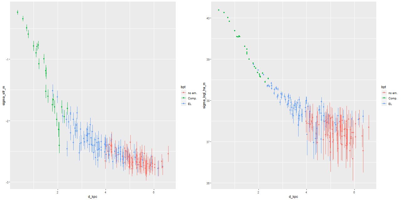
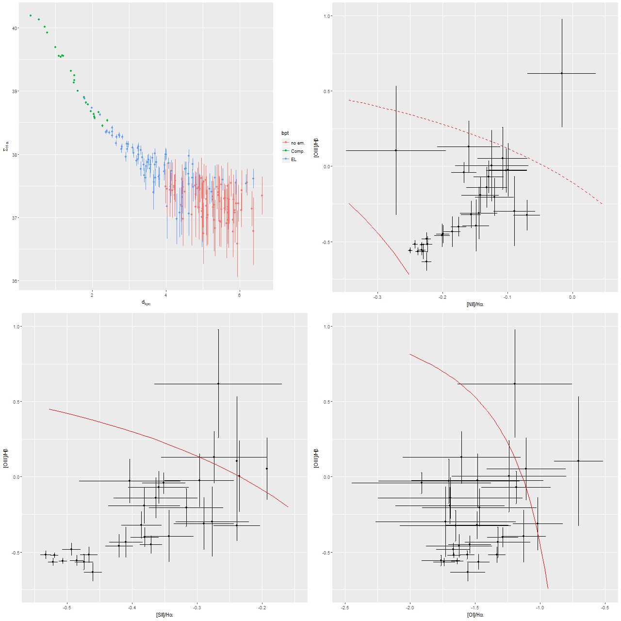
Turning to emission lines, here are the 3 BPT diagnostic diagrams that are most commonly used with SDSS spectra. The curved lines are the starforming/something else demarcation lines of Kewley et al. 2006. In spatially resolved spectroscopy these lines seem not so useful. I find, in agreement with Li et al., that many of the spectra have “composite” line ratios, but except for the central fiber these are mostly near the edge or outside the KDC. The bottom right panel below shows the trend with radius of the [S II]/Hα line ratio (the other two show similar but weaker trends). This trend is the opposite of what we’d expect if an AGN were the ionizing source. Shocks or hot evolved stars are more likely.
Emission line diagnostic (BPT) plots
TL: [N II]/Hα vs [O III]/Hβ
TR: [O I]6300/Hα
BL: [S II]/Hα
BR: trend of [S II]/Hα with radius
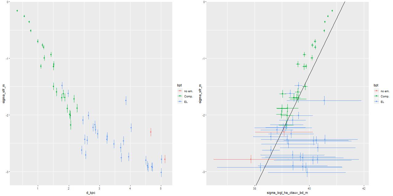
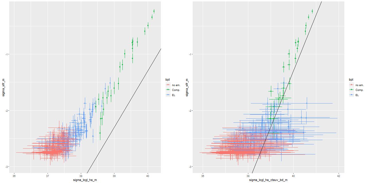
I estimate a 100Myr average star formation rate from the SFH models. The log of the star formation rate density (in \(\mathsf{M}_{\odot}/\mathsf{yr/kpc}^2\)) is plotted against log stellar mass density (in \(\mathsf{M}_{\odot}/\mathsf{kpc}^2\)) below (the line is the estimate of the SF main sequence of Renzini and Peng 2015). Again in agreement with Li et al. the areas of highest SFR lie near the SF main sequence, while the outskirts of the IFU footprint fall below it. log SFR density vs. log stellar mass density
The radial trend of star formation rate is shown below on the left. On the right is my estimate of SFR density plotted against Hα luminosity density along with the calibration of Moustakis et al. Hα is corrected for attenuation using the Balmer decrement.
(L) log SFR density vs. radius
(R) log SFR density vs. attenuation corrected log Hα luminosity density
By the way my models directly estimate dust attenuation of the stellar light, typically assuming a Calzetti attenuation curve. A comparison with attenuation estimated with the Balmer decrement is shown below. To anyone familiar with SDSS spectra it’s not too surprising that estimates from the Balmer decrement have a huge amount of scatter due mostly to the fact that Hβ emission line strength is often poorly constrained. Despite that there is a clear positive correlation between these two estimates. I will probably examine this relationship in more detail in a future post, perhaps based on more favorable data.
τV estimated from Balmer decrement vs SFH model estimates
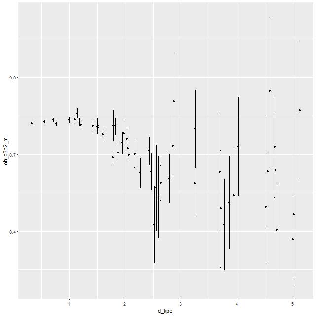
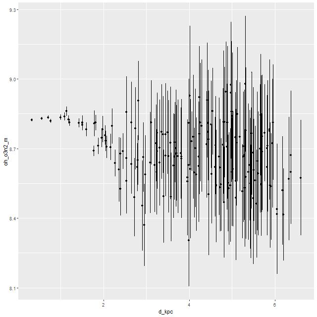
Finally, trend with radius of the metallicity 12+log(O/H) estimated with the strong line O3N2 method. As with the post merger galaxy in the previous posts there is a hint of a weak negative gradient. Overall the gas phase metallicity is around solar or just a little below. This is somewhat lower than my other post merger example, which is not unexpected given an approximately factor of 4 difference in stellar masses.
Metallicity 12+log(O/H) vs radius, estimated by O3N2 index
I’m going to end this series for now with a more detailed look at the spatially resolved star formation history of this galaxy and make a highly selective comparison to some recent theoretical and empirical work on mergers. This continues from part 1 and part 2.
My main theoretical sources for the following discussion include a paper titled “The fate of the Antennae galaxies” by Lahén et al. (2018) and a similar paper also simulating an Antennae analog by Renaud, Bournaud and Duc (2015). I didn’t pick these because I necessarily think this galaxy is an evolved analog of the Antennae; in fact I think there are important differences in the likely precursors. The main reason is these studies are among the first to run very high resolution simulations through and beyond coalescence. Some other significant papers include high resolution simulations with detailed treatment of feedback by Hopkins et al. (2013), Di Matteo et al. (2008), who studied a large sample of merger and flyby simulations, Bekki et al. (2005) who specifically looked at the formation of K+A galaxies through mergers, and Ji et al. (2014) who studied the lifetime of merger features using a suite of simulations. This doesn’t begin to scratch the surface of this literature. Merger simulations are very popular!
Some recent observational papers that examine individual post-merger systems in more or less detail include Weaver et al. (2018) and Li et al. (2018). I will return to the latter paper, which was based on MaNGA data, in a later post. Other observational work that’s more statistical in nature includes Ellison et al. (2015), Ellison et al. (2013), and earlier papers in the same series.
As I’ve mentioned several times already the model spectra I use mostly come from the 2017 EMILES extension of the MILES SSP library with BaSTI isochrones and Kroupa IMF, supplemented with unevolved model spectra from the 2013 update of BC03 models. The results reported in the previous two posts used a small subset of the library — just 3 metallicity bins and 27 time bins, with every other time bin in the full library starting with the second excluded. For my “full” MILES subset I use 4 metallicity bins with \([Z/Z_{\odot}] \in \{-0.66, -0.25, 0.06, 0.40\}\) and all 54 time bins (the lowest metallicity bin is dropped in the reduced subset). Execution time of the Stan SFH models is roughly proportional to the number of parameters, so everything else equal it takes about 2.5 times longer to run a single model with the full set.
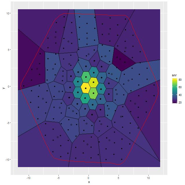
For this exercise I binned the MaNGA spectra with a considerably higher target SNR than usual, ending up with 53 coadded spectra out of the original 183 fiber/pointing combinations. One of the mods I made to Cappellari’s Voronoi binning code was to drop a “roundness” check. The bins in this case still end up with reasonably compact shapes since the surface brightness within the IFU footprint is fairly symmetrical. All but one of the spectra in the inner 2 kpc. ended up unbinned, so the spatial resolution in that critical region is unchanged.
S/N in binned spectra
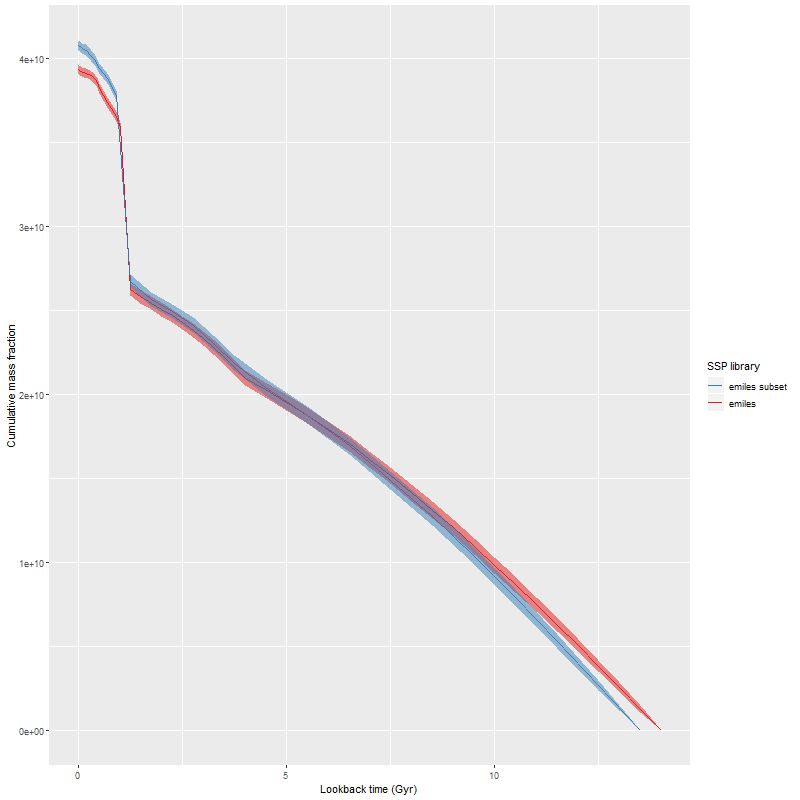
To directly compare the results from the current round of models with the previous lower time resolution runs here are the modeled mass growth histories summed over the entire IFU footprint (blue is the EMILES subset):
Total mass growth histories – emiles subset and full emiles library
Note: MaNGA’s dithering strategy results in considerable overlap in fiber positions in order to obtain a 100% filling fraction. That means the area in fibers exceeds the area of the IFU footprint by about 60%. So, sums of quantities like masses or star formation rates need to be adjusted downwards by about 0.2 dex.
The only real difference we see in the higher time resolution runs is that the initial, strongest starburst is a few percent weaker, and there are some subtle differences in late time behavior. The first large starburst begins at 1.25 Gyr in both sets of runs, and unfortunately this bin is 250 Myr in width in the full resolution set, vs 350 Myr in the subset, so we don’t really get significantly finer grained estimates of the SFH in the initial burst.
We can get a rough idea of the nature of the precursors from this graph. The present day stellar mass is \(4 \times 10^{10} M_{\odot}\), of which just about a third was formed in or after the initial starburst. The present day combined stellar mass of the precursors was just over \(2.6 \times 10^{10} M_{\odot}\) just before the burst — the then stellar mass would have been somewhat larger since this mass growth estimate includes mass loss to stellar evolution. Also, there’s considerable light and therefore stellar mass outside the IFU footprint — the drpcat value for the effective radius is 5.5″ while the Petrosian radius per the SDSS photo pipeline is 12.5″. The IFU footprint is about 10″ radius, or about 1.8 effective radii. Taking a guess that we’re sampling about 80% of the stellar mass the values above need to be adjusted upwards by 25%. Assuming the precursors were equal mass and rounding up their pre-merger stellar masses would be around \(1.65 \times 10^{10} M_{\odot}\). Guessing the current total stellar mass to be \(5 \times 10^{10} M_{\odot}\) then \(1.7 \times 10^{10} M_{\odot}\) was added by the merger. The amount of gas turned into stars was actually higher — about \(2.4 \times 10^{10} M_{\odot}\), but some, maybe most, of the gas lost to stellar evolution might have been recycled. But, I’ll be conservative and adopt the higher value. If that was divided equally between the progenitors they would have had gas masses around \(1.2 \times 10^{10} M_{\odot}\) just before the merger, or just over 40% of the baryonic mass. While high that’s not extraordinarily so for a late type spiral in that stellar mass range (see for example Ellison et al. 2015, figures 6-7).
These values are rather different from the putative Antennae analogs in the two studies linked above, which are in turn rather different from each other. Lahén et al. assign equal stellar masses of \(4.7 \times 10^{10} M_{\odot}\) to each progenitor, equal gas masses of \(0.8 \times 10^{10} M_{\odot}\) (14.5% of the total baryonic mass), and a baryonic to total mass ratio of 0.1. The simulations of Reynaud et al. have stellar masses of \(6.5 \times 10^{10} M_{\odot}\) apiece, gas masses of just \(0.65 ~\mathrm{and}~ 0.5 \times 10^{10} M_{\odot}\), and dark matter halos of \(23.8 \times 10^{10} M_{\odot}\) (for a baryonic to total mass ratio of about 23%). The merger timescales are rather different too: 180 Myr from first pericenter passage to coalescence for the Reynaud et al. simulations vs. ~600 Myr for Lahén et al. (the latter seems closer to the observational evidence; for example Whitmore et al. 1999 found clusters with 3 distinct age ranges up to ~500Myr, with the oldest argued to have formed in the first pericenter passage).
The qualitative features of the merger progress are similar however, and some are fairly generically observed in simulations. There are two pericenter passages, with a second period of separation followed shortly by coalescence at the third pericenter. Star formation is widespread but clumpy in the first flyby, with a large but short starburst and slow decline. A stronger, shorter, and more centrally concentrated starburst occurs around the time of the second pericenter passage through coalescence. The Lahén simulations follow the merger remnant for another Gyr — they show an exponentially declining SFR from an elevated level immediately after coalescence. Neither of these sets of simulations attempt to model AGN feedback, which would presumably cause more rapid quenching. Notably, the Lahén merger remnant develops a kinematically decoupled core although overall the remnant is a fast rotator. Unless the rotation axis is pointing right at us this galaxy is a slow rotator except for the core.
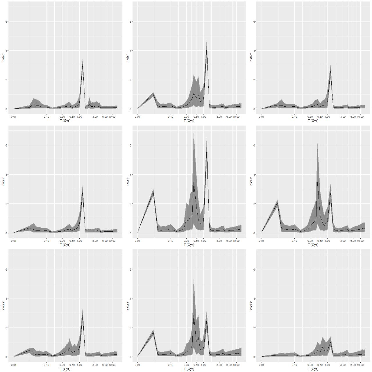
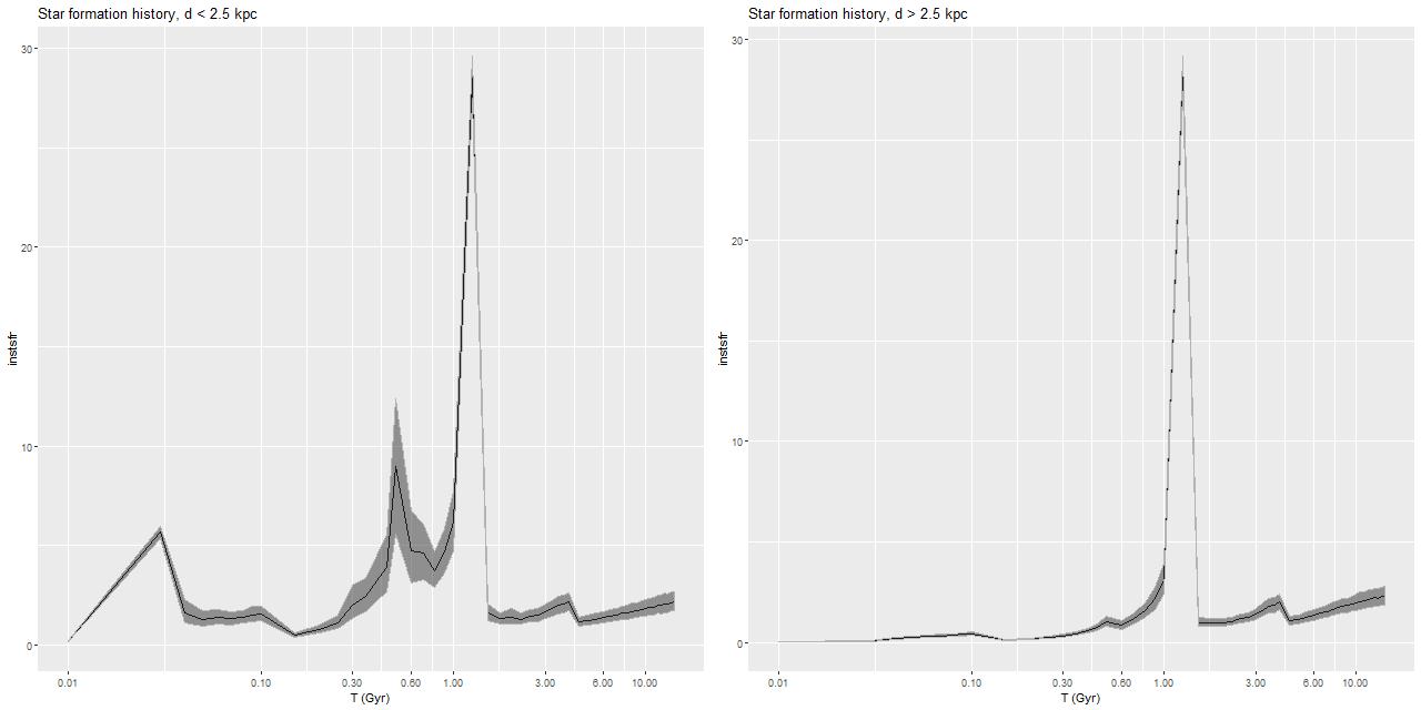
Getting back to data for this galaxy I show some star formation history plots below, first for the inner 9 fibers (all within <1.25 kpc of the nucleus). Below that are a pair of plots of aggregate SFH for fibers within 2.5 kpc (left) of the nucleus and outside that radius (right). The time axis on these plots is logarithmic since I want to focus on the late time behavior (and also this is closer to the real time resolution). Note that in the inner region there are 3 broad peaks in star formation rate — the previously discussed one at 1-1.25Gyr, one centered around 500Myr, and a recent (\(\lesssim\)100Myr revival that peaks at the youngest BaSTI age of 30Myr. The relative and absolute sizes of the peaks are highly variable, indicating that the stars aren’t fully relaxed yet. The outer region covered by the IFU by contrast has just a single peak at 1-1.25Gyr, with a more or less monotonic decline thereafter.
If we believe the models the straightforward interpretation is the first pericenter passage happened about 1-1.25Gyr ago, with coalescence around 500Myr ago and continued infall or recycling driving the ongoing star formation. This is consistent with simulations, which can have merger timescales ranging anywhere from a few hundred Myr to several Gyr. The main problem with this interpretation is that in most simulations the highest peak SFR occurs around coalescence, with the integrated SF roughly equally divided between the first passage and during/after coalescence. In these models about 75% of the post-burst star formation occurs in the 1-1.25Gyr bin, with about 23% in the later burst. An alternative scenario then would be that the entire merger sequence occurred in the 250Myr window of the 1-1.25Gyr bin, and everything since is due to post-merger infall. Of course a third possibility, which I don’t dismiss, is that the details of the modeled episodes of star formation are just artifacts having no particular relationship to the real recent star formation history. The main argument I have against that is that all the spectra seem to tell a consistent story of multiple recent episodes of star formation of varying strength in space and time, and with clear radial trends.
Regardless of the details this galaxy nicely confirms several of the predictions of Bekki et al. (linked above). As we saw in the last post there is a positive color gradient and negative Balmer absorption gradient as they predict for dissipative major mergers, with a break in the color gradient trend that corresponds approximately with the boundary between multi-peaked and single peaked late time star formation histories.
The obvious morphological indicators of disturbance are provocative but don’t seem to be highly constraining. My recollection is that folklore guesstimates that tidal features have a visible lifetime of ~1 Gyr. Ji et al. (linked above) on the other hand found based on a suite of simulations that merger features remain visible at the 25 mag./arcsec\(^2\) somewhat longer, on average about 1.4Gyr. It may be significant that the disturbance is easily seen even in the SDSS Navigate imaging, especially the northern loop. The somewhat similar star forming elliptical SDSS J1420555.01+400715.7 discussed by Li et al. (which I will turn to later) required deeper imaging and some enhancement to show signs of disturbance. One thing I’m working on learning is galaxy profile fitting and photometric decomposition. I’d like to see if the single component Sersic fit that fit the mass density profile also works for the surface brightness (I suspect there is a steeper core). I’d also like to quantify the surface brightness in the tidal features. These are exercises for later.
Star formation histories estimated from innermost 9 spectra (d < 1.25 kpc)
Binned star formation histories (full SSP library) L – d ≤ 2.5 kpc R – d > 2.5 kpc
I’m going to conclude with a few plots of quantities that I thought might benefit from the higher S/N in the binned spectra. First is the gas phase metallicity from the O3N2 index plotted against radius. Unfortunately emission line strengths are still too weak beyond about 2.5 kpc radius to say much about the outskirts, but we still see a fairly flat trend with radius up to ~1.5 kpc with a turnover to lower values that continues at least out to ~2.5kpc. This is broadly similar with the simulations of Lahén et al., who obtained a shallower metallicity gradient for their merger remnant than an undisturbed spiral galaxy.
gas phase metallicity 12 + log(O/H) vs radius, estimate from O3N2 index. Binned spectra
Here I again plot the estimated SFR density against radius and the estimated SFR density against Hα luminosity density. The high luminosity end is essentially unchanged from the plot in the last post since these spectra are unbinned. Again, the points at the high luminosity end lie above the Hα-SFR calibration of Moustakas et al. by considerably more than the nominal length of the error bars, which points to a likely recent (< ~10Myr) fading of star formation. This is consistent with the detailed SFH models. At the other end of the luminosity scale there seems to be an excess of points to the right of the calibration line. This could indicate that the main ionization source in the outer regions of the IFU footprint is something other than massive young stars (presumably shocks or hot evolved stars).
L – SFR density vs. radius R – SFR density vs. Hα luminosity density Binned spectra with enlarged EMILES SSP library
Despite the “composite” emission line ratios in the central region there’s little evidence for an AGN. The galaxy is a compact FIRST radio source, but the size of the starforming region is right around the FIRST resolution. The raw WISE colors are W1-W2 = +0.07, W2-W3 = +2.956, which is well within the locus of spiral colors.
In part two of this series that I began here I’m going to look at various quantities derived from the modeled star formation histories and emission line fits. Later I’ll dive into some selected recent literature on major gas rich mergers and do some comparisons. I’m especially interested in whether the model star formation histories have anything to tell us about the chronology of the merger and the nature of the progenitors.
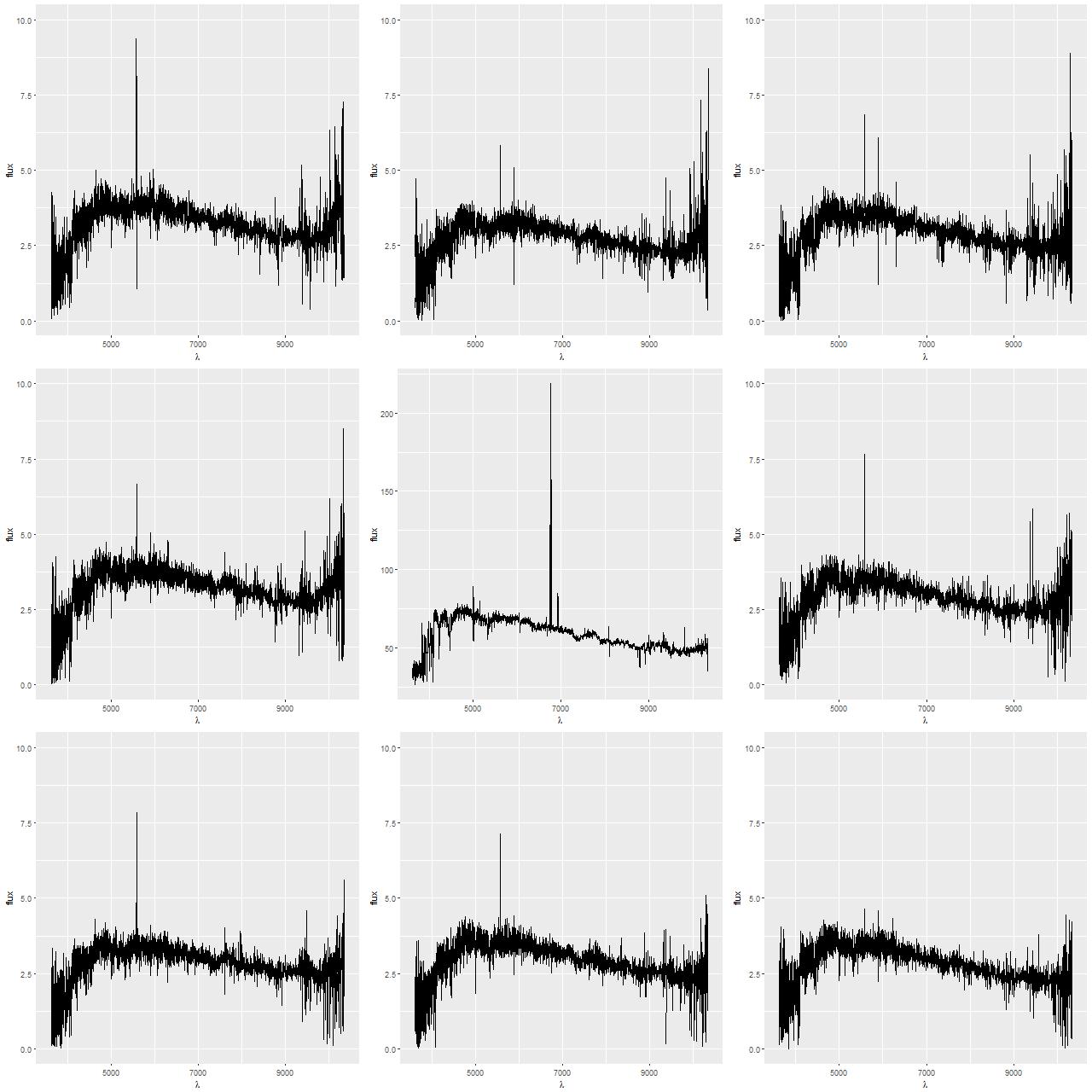
First, here is a representative sample of spectra. These are reduced to the local rest frame and fluxes are corrected for foreground galactic extinction but not any internal attenuation. The middle spectrum in the second row is from the central fiber/pointing combination (remember these are from the stacked RSS data). The peripheral spectra are roughly equally spaced along a ring about 7″ or 4kpc from the center.
The central spectrum does show moderately strong emission lines along with fairly strong Balmer absorption, which points to some ongoing star formation along with a significant intermediate age population. Emission lines are evidently lacking or very weak in the peripheral spectra (most of the spikes are terrestrial night sky lines or simply noise), indicating the galaxy is currently passively evolving at 4kpc radius. In more detail…
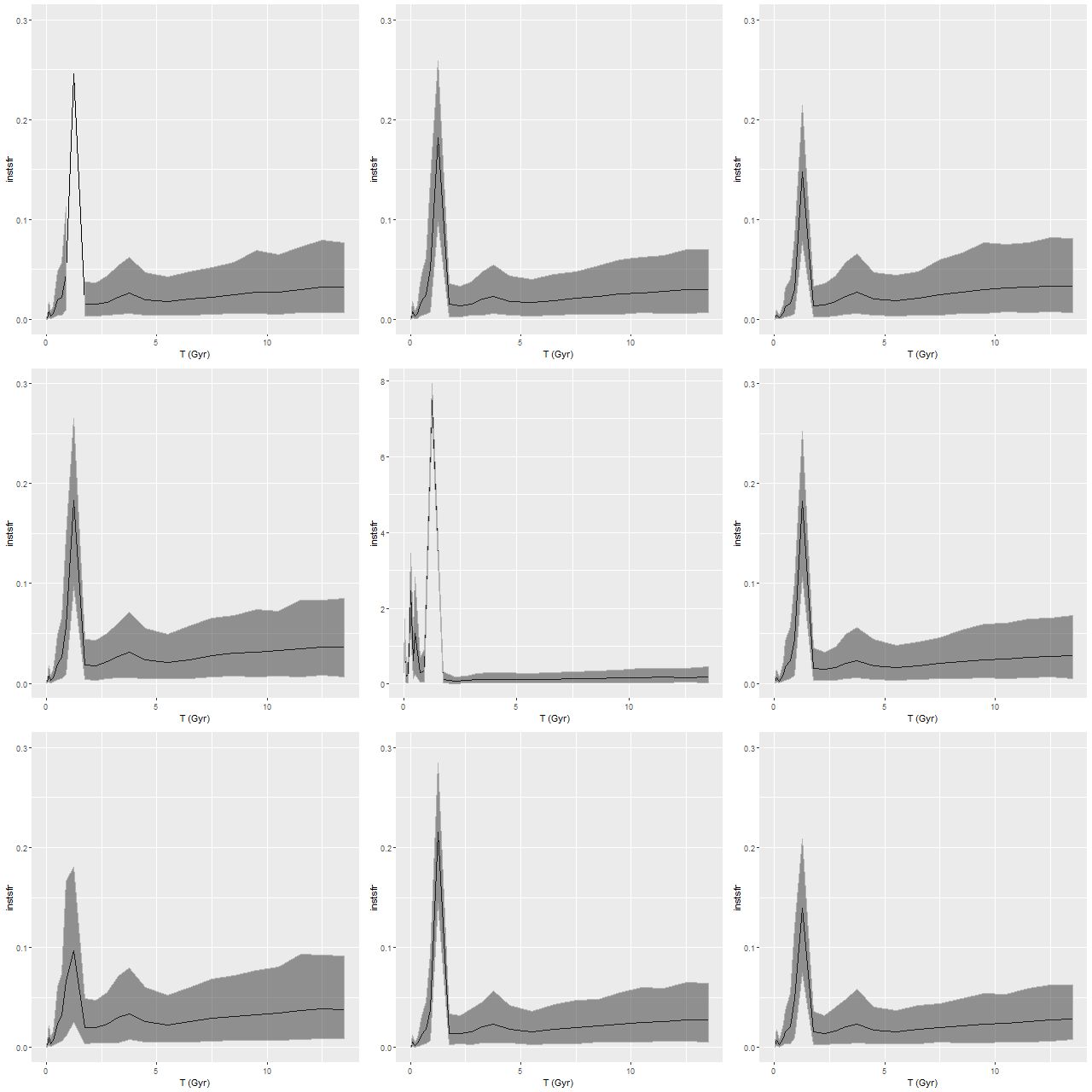
The most basic but also finest grain quantities I look at are posterior estimates of star formation histories and mass growth histories. These contain similar, but not quite the same information content. I show star formation histories as the “instantaneous” star formation rate vs. look back time defined as the total stellar mass born in an age bin divided by its width in years.
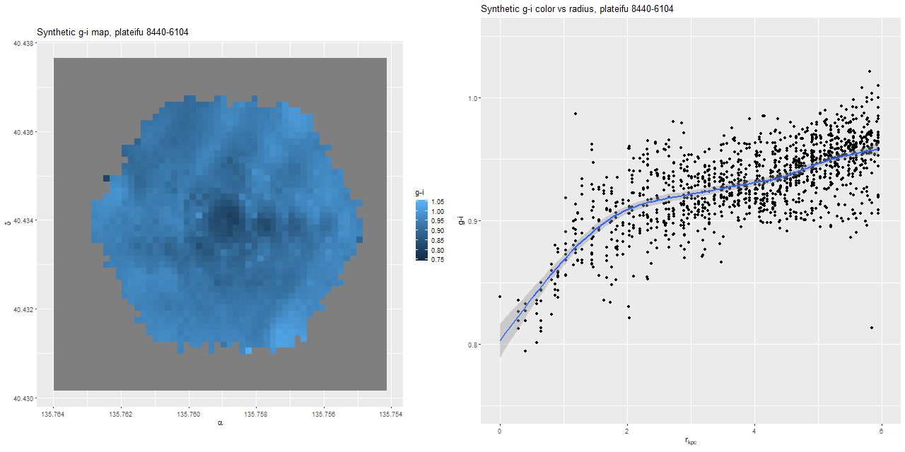
Sample star formation histories – plateifu 8440-6104, mangaid 1-216976
Mass growth histories estimate the cumulative fraction of the present day stellar mass. These incorporate a recipe for mass loss to stellar evolution and as such aren’t quite integrals of the star formation histories. By convention remnant masses are included in stellar mass, and there are recipes for this as well (in this case taken from the BaSTI web page). I display posterior marginal means and 95% confidence intervals for both of these against time.
I think I first encountered empirical estimates of mass growth histories in McDermid et al. (2015), although earlier examples exist in the literature (eg Panter et al. 2007). I may be the first to display them for an individual galaxy at the full time resolution of the input SSP library. Most researchers are reluctant to make detailed claims about star formation histories of individual galaxies based on SED modeling. I’m not quite so inhibited (not that I necessarily believe the models).
Sample mass growth histories — plateid 8440-6104
The most obvious feature in these is a burst of star formation that began ≈1.25 Gyr ago that was centrally concentrated but with enhanced star formation galaxy wide (or at least IFU footprint wide). In the central fiber the burst strength was as much as 60%, with the amplitude fading away with distance. Is this percentage plausible? First, just summing over all fibers the mass formed during and after the initial burst is about 1/3 of the present day stellar mass. This probably overestimates the burst contribution since the galaxy extent is considerably larger than the IFU and the outer regions of the progenitors likely experienced less enhanced star formation, but even 1/3 is consistent with the typical neutral hydrogen content of present day late type spirals. I will look at the merger simulation literature in more detail later, but simulations do predict that much of the gas is funneled into the central region of the merger remnant where it’s efficiently converted into stars, so this is broadly consistent with theory. But second, I have some evidence from simulated star formation histories that the presence of a late time burst destroys evidence of the pre-burst history, and this leads to models underestimating the early time mass growth. This could have an ≈0.1 dex effect on the total stellar mass estimate.
Most of the SFH models show more or less monotonically declining star formation rates after the initial burst, but the central fiber shows more complex late time behavior with several secondary peaks in star formation rate. It’s tempting to interpret these literally in hopes of constraining the timeline of the merger. In the next post I’ll look at this in more detail. One limitation of this set of models is the coarse time resolution. I only used half the available SSP ages from the EMILES/BaSTI library — the critical 1.25Gyr model in particular is 350Myr wide, which is a significant fraction of the expected timescale of the merger. Next time I’ll look at the results of some higher time resolution model runs.
I look at a large and still growing number of quantities derived from the models. For visualization it’s sometimes useful to create maps like the ones I showed in the first post on this galaxy. Many interesting properties of this particular galaxy are fairly radially symmetric with strong radial trends, so simple scatter plots are most effective.
I posted several graphs in a post on the current GZ Talk. Since those posts I’ve learned how to do Voronoi binning by translating Cappellari’s Python code to R. I also noticed that some of the EMILES spectra are truncated in the red within the range I was using for SED fitting, so I trimmed it to a wavelength range with strictly positive model fluxes (currently rest frame wavelengths 3465-8864 Å) and reran the models on the binned data. Binning has little effect on the results since out of 183 fiber/pointing combinations I ended up with 179 binned spectra. There are small changes due to the reduced wavelength range.
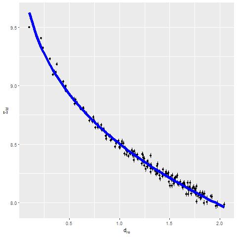
One of the more interesting plots I posted there was the estimated stellar mass density (in log solar masses/kpc^2) against radius (measured in effective radii; the effective radius from the drpall catalog is 5.48″ or about 3.2 kpc). The updated plot is below. The blue line is a single component Sersic model with Sersic index n=3.35 from a nonlinear least squares fit using the R function nls() (no Bayes this time). This is close enough to a deVaucouleurs profile (n=4) and definitely not disky (n=1). I will someday get around to comparing this to a photometric decomposition — they should be similar, although this fit is undoubtedly affected by the low spatial resolution of the IFU data.
Stellar mass density vs. radius in effective radii with single component Sersic fit plateid 8440-6104, mangaid 1-216976
The other plots I posted there included the star formation rate density (in \(M_\odot/yr/kpc^2\), averaged over an arbitrarily chosen 100 Myr) against radius and Hα luminosity density (uncorrected for internal attenuation) against radius:
Star formation rate density and Hα luminosity density against radius
The trends look rather similar, which leads to the obvious (SFR density vs. luminosity density):
Star formation rate vs. Hα luminosity. L uncorrected for attenuation; R corrected via Balmer decrement
This is one of the more remarkable and encouraging results of these modeling exercises — the star formation rate estimates come entirely from the stellar component fits and are for an order of magnitude longer time scale than is probed by Hα emission. Optical SED fitting is rarely considered suitable for estimating the recent star formation rate, yet we see a tight linear relationship between the model estimates and Hα luminosity, one of the primary SFR calibrators in the optical, that only begins to break down at the lowest luminosities. In the right pane Hα is corrected for attenuation using the Balmer decrement with an assumed intrinsic Hα/Hβ ratio of 2.86. The straight line in both graphs is the Hα-SFR calibration of Moustakas, Kennicutt, and Tremonti (2006) with a 0.2 dex intercept shift to account for different assumed IMFs. At the well constrained high luminosity end most of the points appear to lie above the relation, which could indicate that recent star formation has declined relative to the 100Myr average (or of course it could be a fluke).
Two other measures of star formation rate I track are specific star formation rate, that is SFR divided by stellar mass (which has units of inverse time), and relative star formation rate, SFR divided by the average SFR over cosmic time. Trends with radius (note that these and just about all other quantities I track are scaled logarithmically):
SSFR and relative star formation rate
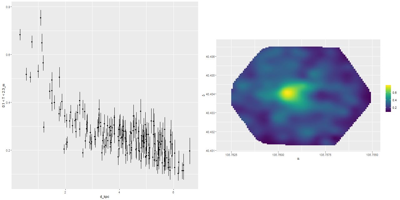
On longer time scales I track the stellar mass fraction in broad age bins (this has been the customary sort of quantity reported for some years). Here is the intermediate age mass fraction (0.1 < T ≤ 2.3 Gyr), which basically measures the burst strength for this galaxy:
Burst mass fraction – trend and map
Oddly, the peak burst strength is somewhat displaced from the photometric center.
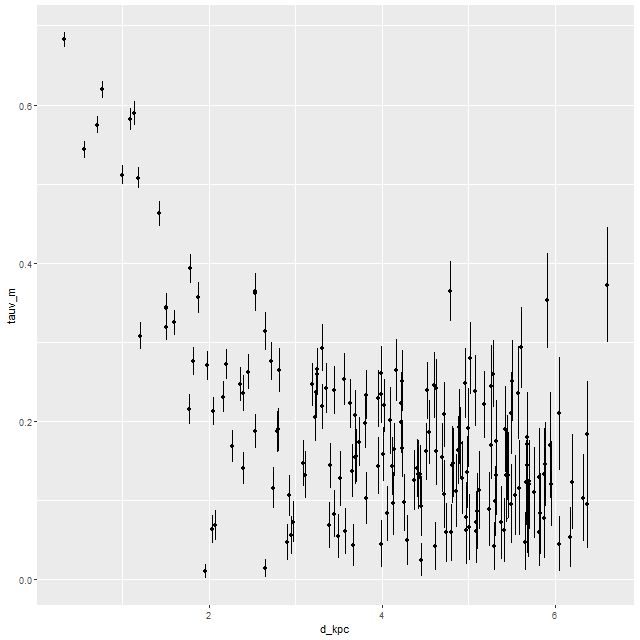
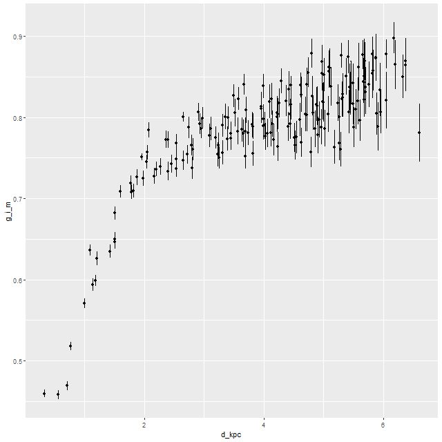
For completeness, here are trends of the modeled optical depth of stellar attenuation and intrinsic g-i color (a long wavelength baseline color serves as a rough proxy for specific star formation rate):
Optical depth of stellar attenuation
This is very similar to the color trend calculated from the spectral cubes I showed in the first post.
Model intrinsic g-I color trend
Finally, in recent months I have begun to track several “strong line” gas phase metallicity indicators. Here is an oxygen abundance estimate from the O3N2 index as calibrated by Pettini and Pagel (2004). Astronomers present “heavy” element abundances in the peculiar form 12 + log(O/H) where O/H is the number ratio of Oxygen (or other element) to Hydrogen.
Oxygen abundance 12 + log(O/H) by O3N2 index
Unlike just about everything else there’s no clear abundance trend here, although the precision drops dramatically outside the central few kpc. For reference the solar Oxygen abundance (which is surprisingly unsettled) is around 8.7, so the gas phase metallicity is around or perhaps a little above solar.
So, to summarize, there was a powerful burst of star formation that began ~1Gyr ago that was clearly triggered by a gas rich major merger. The starburst was centrally concentrated but enhanced star formation occurred galaxy wide (perhaps not uniformly distributed). Star formation is ongoing, at least within the central few kiloparsecs, although there is some evidence that it is fading now and is certainly much lower than the peak.
The stellar mass distribution is elliptical-like although perhaps not quite fully relaxed to a new equilibrium. As we saw in the previous post there is no evidence of regular rotation, although there is a rotating kinematically decoupled core that coincides in position with the region where the starburst was strongest.
Next post I’ll look at some of the recent merger literature, and also show some results from higher time resolution modeling.
As I mentioned in the first post I’ve been doing star formation history (SFH) modeling by full spectrum fitting of galaxy spectra for several years. I’m going to quickly review what I do as a prelude to the next several posts where I plan to look at my proto-K+A galaxy in more detail. I’ll probably return to modeling details in the future. I still haven’t reached the point of having version controlled code let alone “publishing” it, but that’s not far off (I hope).
Full spectrum fitting is actually pretty simple, especially since other people have already done the hard work. The basic observational data is a set of monochromatic fluxes \(g_{\lambda}\) with estimated uncertainty at each point \(\lambda\) (\(\lambda\) is just a discrete valued index here) \(\sigma_{\lambda}\) or precision (inverse variance) \(p_{\lambda} = 1/\sigma^2_{\lambda}\) . For now let’s assume that observed fluxes are independently gaussian distributed with known variances (yes, this is a simplification).
The second main ingredient is a set of template spectra \(T_{\lambda, n}, n = 1, \ldots, N\), which nowadays usually comprises model spectra from a library of simple stellar population (SSP) models. If the physical parameters of the templates span those of the galaxy being modeled its spectrum would be fit with some nonnegative combination of the template spectra:
and by assumption the errors \(\epsilon_{\lambda}\) are gaussian distributed with mean 0 and standard deviation \(\sigma_{\lambda}\).
The spectroscopy we deal with is high enough resolution to be blurred by the constituents of the galaxy, so an additional ingredient is the “line of sight velocity distribution” (LOSVD), which must be convolved with the templates. Finally, it’s common to include additive or multiplicative functions to the model to allow for calibration variations or to model attenuation. I hopefully assume calibrations are well matched between observations and models and only attempt to model attenuation, usually with a Calzetti relation parametrized by optical depth. So, the full model looks like:
where the \(v_n\) are (possibly vector valued) parameters of the LOSVD and \(\tau_{V,n}\) is the dust optical depth at V. These are nominally indexed by n to indicate that there may be different values for different model constituents. In practice I only consider a few distinct components.
An important insight of Cappellari and Ensellem (2004) that was dismissed in two sentences is that conditional on the parameters of the LOSVD and any multiplicative factors the subproblem of solving for the coefficients \(\beta_n\) is a linear model in the parameters with nonnegativity constraints, for which there is a fast, deterministic least squares algorithm due originally to Lawson and Hanson (1974). This greatly simplifies the nonlinear optimization problem because whatever algorithm is chosen for that only needs to optimize over the parameters of the LOSVD and optical depth. I currently use the general purpose optimization R package Rsolnp along with nnls for SED fitting. This is all similar to Cappellari’s ppxf but less versatile; my main interest is in star formation histories and I’ve found a better way to estimate them in a fully Bayesian framework. These days I mostly use the maximum likelihood fits as inputs to the Bayesian model implemented in Stan.
I have used several SSP libraries, but the workhorses recently have been subsets of the EMILES library with BaSTI isochrones and Kroupa IMF, supplemented with some unevolved models from BC03. One thing I do that’s not unprecedented but still somewhat unusual is to fit emission lines simultaneously with the stellar library fits. I do this by creating fake emission line spectra, one for each line being fit (usually the lower order Balmer lines and selected forbidden lines).
The models that I’m likely to discuss for the foreseeable future use separate single component gaussian fits to the stellar and emission line velocity distributions. I assume the velocity offsets calculated in the first step of the analysis are accurate, so the mean of the distributions is set to 0. I also use a single component dust model, usually with Calzetti attenuation relation. I don’t try to tie the relative strengths of emission lines, so attenuation is only directly modeled for the stellar component. These assumptions are obviously too simple for galaxies with broad emission line components or interacting galaxies with overlapping stellar components. For now I plan to ignore those.
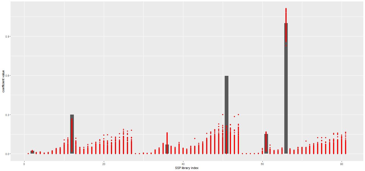
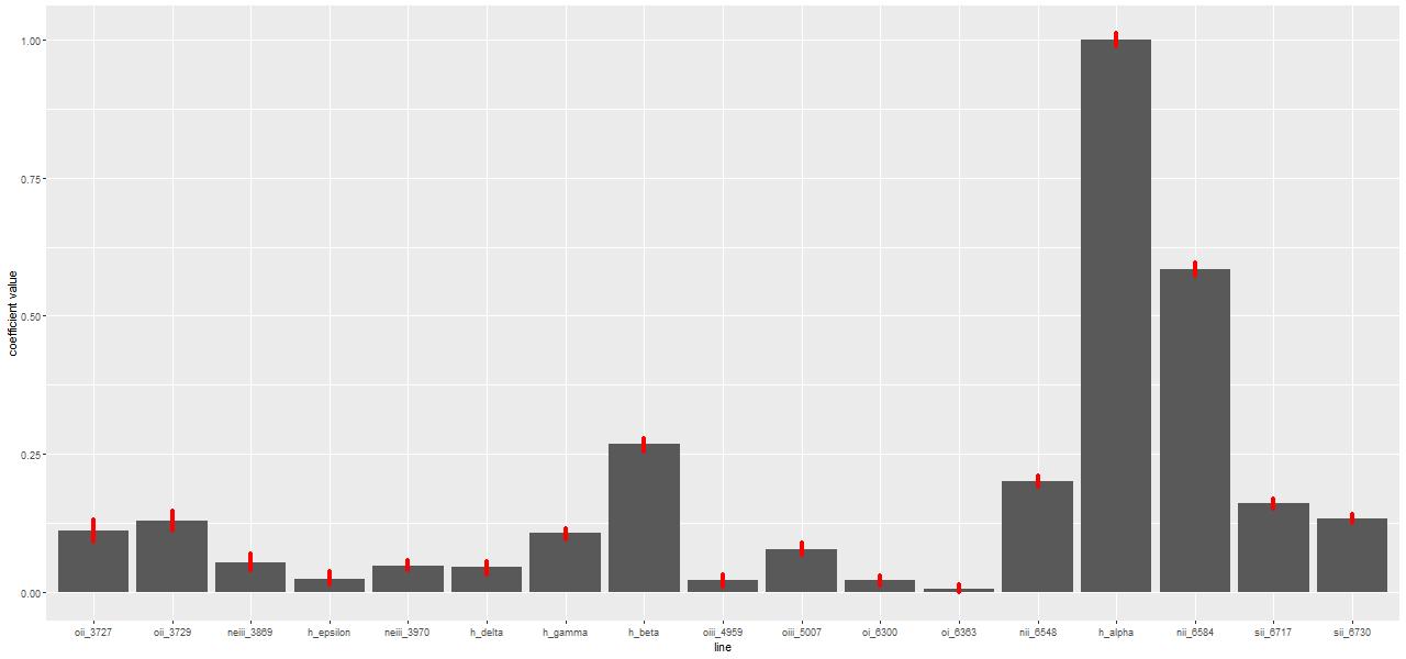
One interesting property of the NNLS algorithm for this application is that it always returns a parsimonious solution for the stellar component, with usually only a handful of contributors. An example of a solution from a fit to the central spectrum of the proto-K+A galaxy I introduced a few posts ago is shown below. The grey bars are the optimal contributions (proportional to the mass born in each age and metallicity bin) from the elements of the SSP library. This particular subset has 3 metallicity bins and 27 age bins ordered from low to high.
Only six (actually a seventh makes a negligible contribution) SSP model components are in the optimal fit, out of 81 in this particular library. Usually in statistics sparsity is considered a highly desirable property, especially in situations like this with a large number of explanatory variables. Considerable effort has been made to derive conditions where non-negative least squares, which has no tuning parameters, automatically produces sparse solutions (see for example Meinshausen 2013). However in this context sparsity is maybe not so desirable since we expect star formation to vary continuously over time in most cases rather than in a few short bursts as would be implied here: as a Bayesian my prior assigns positive probability density to star formation at all times.
But in the absence of a parametric functional form for star formation histories a fully Bayesian treatment of SED modeling is an extremely difficult problem. The main issue is that model spectra are highly correlated; if we could visualize the N dimensional likelihood landscape we’d see a long, curving, steep sided ridge near the maximum. I’ve tried a number of samplers over the years including various forms of Metropolis-Hastings and the astronomers’ favorite EMCEE and none of them are able to achieve usable acceptance rates. A few years ago I discovered that the version of “Hamiltonian Monte Carlo” (informally called the No U-Turn Sampler, or NUTS) implemented in the Stan modeling language is capable of converging to stationary distributions in a tractable amount of time. In the plot below the red dots indicate the range of values taken by each SSP model contribution in the post-warmup sample from a Stan run. Now all time and metallicity bins are represented in the model in amounts that are at least astrophysically plausible. For example instead of a single old component as in the NNLS fit the pre-burst history indicates continuous, slowly declining star formation, which is reasonable for the likely spiral progenitors.
Sample non-negative maximum likelihood SSP fit to full spectrum and Stan fit compared
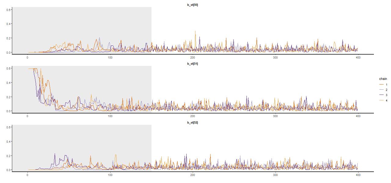
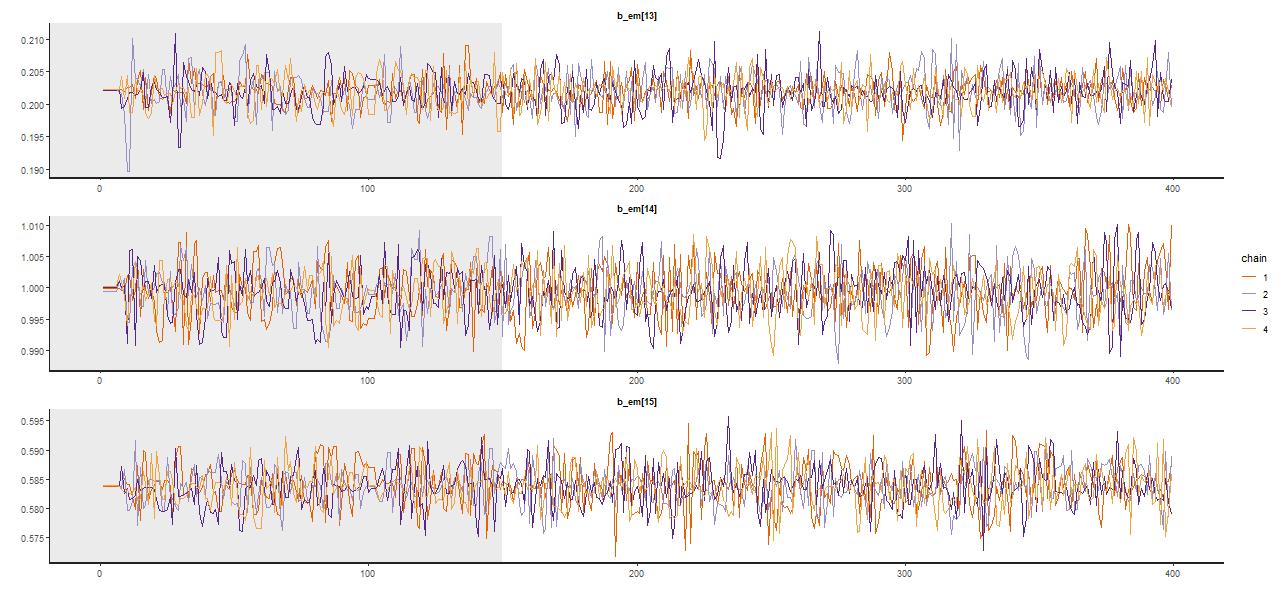
A trace plot, that is a sequential plot of each draw from the sampler, is shown for a few parameters below — these are the single old component in the maximum likelihood fit and the two in the surrounding age bins. Samples spread out rather quickly from the initialized values at the MLE, reaching in this case a stationary distribution about 2/3 of the way through the adaptation interval shown shaded in gray; I used a rather short warmup period of just 150 iterations for this run (the default is 1000, while I generally use 250 which seems adequate). There were 250 post warmup iterations for each of 4 chains in this run. No thinning is needed because the chains show very little autocorrelation, making the final sample size of 1000 adequate for inference. Most physical quantities related to the stellar contributions involve weighted sums of some or all coefficients, and these typically show little variation between runs.
Sample traceplot from Stan run
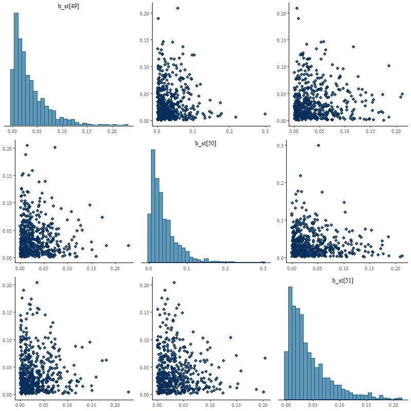
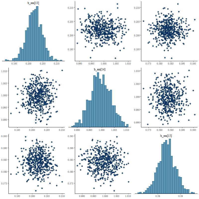
Posterior marginal distributions often have very long tails as shown here. This can be a problem for MCMC samplers and Stan is quite aggressive in warning about potential convergence issues. The quantities that I track tend to have much more symmetrical distributions.
Sample marginal posterior distributions of stellar contributions
Fits to emission lines tend to behave differently. If they’re actually present the MLE will have positive contributions (the coefficients are proportional to emission line fluxes). On the other hand in a passively evolving galaxy with no emission lines the MLE estimate is typically sparse, that is coefficient estimates will tend to be 0 rather than spuriously small positive values.
Example maximum likelihood fit of emission lines compared to Stan fit
Sample values from Stan tend to stay centered on the ML fits (Hα and the surrounding [N II] lines are shown here):
Sample trace plot of emission line contributions
Marginal posterior distributions tend to be symmetrical, close to Gaussian, and uncorrelated with anything else (except for the [O II] 3727-3729Å doublet, which will have negatively correlated contributions).
Sample marginal posterior distributions of emission line contributions
One thing that’s noteworthy that I haven’t discussed yet is that usually all available metallicity bins make contributions at all ages. I haven’t been able to convince myself that this says anything about the actual distribution of stellar metallicities, let alone chemical enrichment histories. In recent months I’ve started looking at strong emission line metallicity indicators. These appear to give more reliable estimates of present day gas phase abundances, at least when emission lines are actually present.
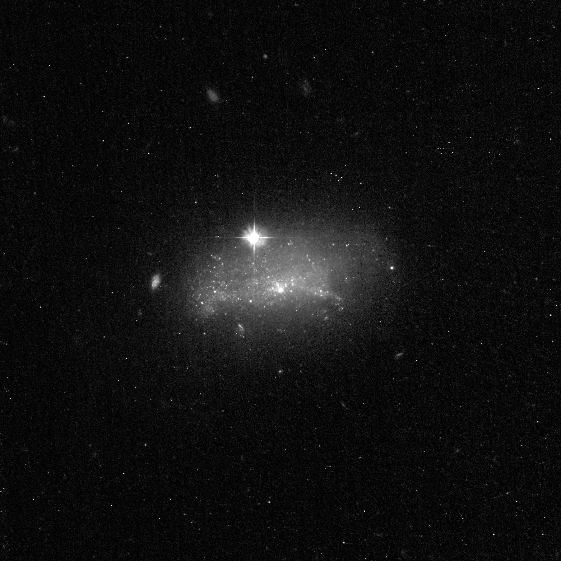
I may as well post this here too. This HST ACS/WFC image was taken as part of SNAP program 15445, “Gems of the Galaxy Zoos,” PI Bill Keel with numerous collaborators associated with Galaxy Zoo (see also this Galaxy Zoo blog post). This is my Q&D processing job on the calibrated/distortion corrected fits file using STIFF and a bit of Photoshop adjustment.
CGCG 292-024 HST/ACS F475W Proposal ID 15445 “ZOOGEMS”, PI Keel
Comparing that to the finder chart image from SDSS below, which is oriented slightly differently, it appears the area observed spectroscopically was a centrally located star cluster or maybe complex of star clusters.
CGCG 292-024 SDSS finder chart image with spectrum location marked
What interested me about this and a number of other nearby galaxies (which were discussed at some length on the old Galaxy Zoo Talk) is it has a classic K+A spectrum:
SDSS spectrum of central region of CGCG 292-024
that the SDSS spectro pipeline erroneously calls a star with an improbably high radial velocity of ≈1200 km/sec. Well it’s not a foreground star obviously enough, and the SDSS redshift is close but not quite right. I measure it to be z = 0.0043, or cz = 1289 km/sec, which agrees well enough with the NED value of 1282 km/sec (obtained from an HI radial velocity by by Garcia et al. 1994).
Karachentsev, Nasonova, and Curtois (2013) assign this galaxy to the NGC 3838 (which is just NW of our target galaxy) group, which they place in the background of the Ursa Majoris “cloud,” which is in turn a loose conglomerate of 7 groups about 20 Mpc. distant. They adopt a distance modulus to the group of 32.3 mag., which is a little higher than the NED value (with H0 = 70 km/sec/Mpc) for this galaxy of 31.6 mag. SDSS lists the g band psfMag as 18.7 for the spectroscopic target, which makes its absolute magnitude around -12.9.
In contrast to the appearance of the spectrum the galaxy itself doesn’t look like a typical K+A galaxy. In the local universe most field or group K+A’s are disturbed ellipticals, which are thought to be the aftermath of major gas rich mergers. This galaxy, while irregular in morphology, is not particularly disturbed in appearance and shows no sign of having recently merged. Quenching mechanisms that are thought to act in cluster environments aren’t likely to be effective here since the Ursa Majoris complex isn’t especially dense (and according to the above authors also light on dark matter). I think I speculated online that this and galaxies like it might actually be old and metal poor (having the infamous “age-metallicity” degeneracy in mind), but that doesn’t really work. Even the most metal poor galactic globular clusters are considerably redder than the spectroscopic object.
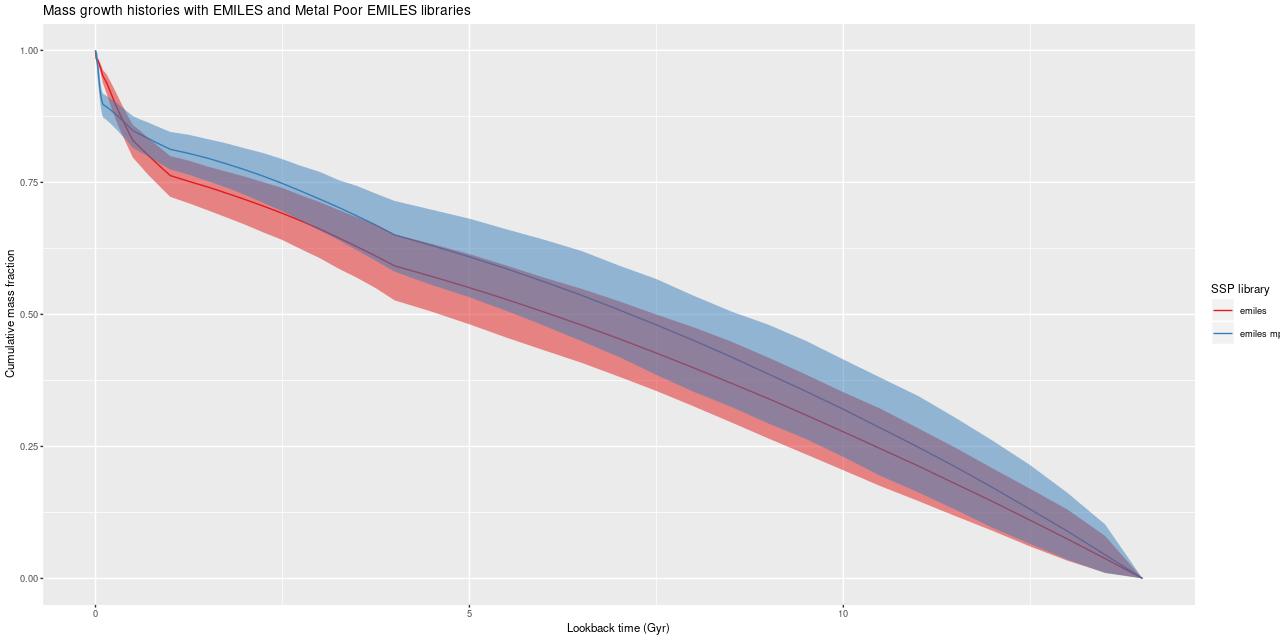
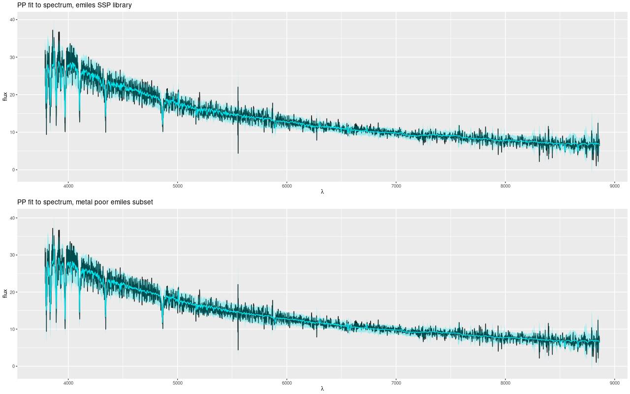
So, I did some SFH modeling, which I will describe in more detail in a future post. I currently mostly use a subset of the EMILES SSP library with Kroupa IMF, BaSTI isochrones and 4 metallicity bins between [Z/Zsun] = -0.66 and +0.40. I supplement these with unevolved models from BC03 matched as nearly as possible in metallicity. For this exercise I also assembled a metal poor library from the Z = -2.27, -1.26, and -0.25 models with all available ages from 30Myr to 14Gyr. Here are estimated mass growth histories:
Estimated mass growth histories, EMILES and metal poor EMILES
Both models have nearly constant rates of mass growth over cosmic history which implies slowly declining star formation, with the metal poor models having slightly faster early mass growth (and hence slightly older light weighted age). Neither exhibits a starburst, faded or otherwise. The “metal rich” model fits show a slight acceleration beginning about 1Gyr ago, while the “metal poor” fits have a few percent contribution from the youngest, 30Myr, population (which already has quite strong Balmer absorption). So the age-metallicity degeneracy manifests in these full spectrum fitting models as small(ish) variations in detailed star formation histories. The fits to the data are indistinguishable:
Posterior predictive fits to SDSS spectrum of central region of CGCG 292-024
The fits to the Balmer lines appear to be systematically weak but this seems to be an artifact. Zooming in on the blue end of the spectrum the posterior predictive fits match the full depth of the absorption lines (Balmer lines from Hγ to Hη are marked)[1]:
Posterior predictive fit to blue part of spectrum
While weak there is some ionized gas emission (note for example that Hα is completely filled in, which implies the emission equivalent width is ~several Å). Here are BPT diagnostic plots for [N II]/Hα, [S II]/Hα, and [O I]/Hα vs [O III]/Hβ. The contours indicate the joint posterior density of the line ratios with arbitrary spacing. The lines are the usual SF/something else demarcation lines from Kewley et al. Although the constraints aren’t very strong most of the probability mass lies outside the starforming region, suggesting that the area sampled by the fiber is at least for now “retired.”
The BR panel of the plot shows the estimated posterior distribution of the “strong line” metallicity indicator O3N2 with the calibration of Pettini & Pagel (2004). This does indicate that the gas-phase metallicity is sub-solar by about 0.6 dex.
BPT diagnostics and strong line metallicity estimate for CGCG 292-024
Conclusion?: I think we’re most likely seeing the effect of stochastic star formation (in time and maybe space as well). The region sampled by the fiber has an estimated (by me) stellar mass slightly lower than \(10^7 M_{\odot}\), which is probably low enough for supernova feedback to at least temporarily suppress star formation. Without more data it’s hard to tell if star formation is globally suppressed at present, but there’s no real reason to think it is. There is a supply of neutral Hydrogen available (see Garcia et al. linked above and Serra et al. 2012), so star formation could well resume any time.
This isn’t quite an accidental “discovery.” There’s been a fair amount of interest in recent years in finding “transitional” galaxies that are rapidly shutting down star formation but that don’t meet the traditional criteria for K+A galaxies (see for example Alatalo et al. 2014, 2016; Wild et al. 2007 among many others). A while back I made my own effort at assembling a sample of post-starburst candidates by looking for spectra in SDSS with strong Hδ absorption and emission line ratios other than starforming in the MPA data tables. This sample had some thousands of candidates, of which there are just 26 in the first two MaNGA data releases. As many as half of those were false positives, which is a little too high, so it’s back to the drawing board. But there were a few interesting hits:
KUG 0859+406 image cutout from legacysurvey.org
This legacysurvey.org cutout (from the MzLS+BASS surveys) shows clearly a pair of tidal tails and some shells, clear signs of a recently consummated merger. The region covered by the IFU footprint on the other hand looks rather featureless:
Plateifu 8440-6104 (mangaid 1-216976) SDSS cutout with IFU footprint
In the remainder of this post I’ll look at a few measured, not too model dependent, properties of the IFU data. In future post(s) I’ll look at the results of star formation history models and other model dependent properties. One thing I’m interested in learning more about is if SFH models of merger remnants tell us anything about the chronology of mergers. We’ll see!
MaNGA data cubes include synthesized griz images created by projecting the spectra onto the filter transmission functions at each spaxel. Below is a g-i color map from these synthetic images, with the color corrected for galactic extinction but not any internal attenuation that might be present. There are hints of structure that indicate the merger remnant hasn’t quite reached equilbrium, but more importantly there is a clear positive color gradient with radius as seen on the right, with a turnover in the slope of the gradient at ≈2 kpc. A positive color gradient is the opposite of what would be seen in a normal disk galaxy, but exactly what we’d expect from the aftermath of a major merger with a centrally concentrated starburst.
L: Synthetic g-i map from IFU data cube, plateifu 8440-6104 (mangaid 1-216976) R: g-i color trend with radius
Several measured quantities are shown below. The input data for these were the stacked RSS files, with the measurements interpolated onto a fine grid for visualization. The velocity field (top left) has several interesting features. First, there is no apparent overall rotation, but the symmetrical pair of lobes with opposite velocity signs just outside the nucleus indicate the presence of a rotating disk or torus. These are known as “kinematically distinct cores” and are somewhat common in early type galaxies (for example Krajnovic et al. 2011), and are expected in some cases in major gas rich mergers (eg Bekki et al. 2005).
The other three panes of this plot are the equivalent width in absorption of the Balmer line Hδ (TR), the 4000Å break strength D\(_n\)(4000) (BL), and Hα emission equivalent width (BR). Hδ is a measure of Balmer absorption line strength and is sensitive to the presence of an intermediate age population. A threshold of around 5Å is usually used to select post-starburst galaxies (eg Goto 2005). My measured peak line strength is \(6.5 \pm 0.2 \)Å (the same as the MPA estimated emission corrected value for the SDSS fiber spectrum), and the inner \(\approx 1.5\) kpc. has Hδ > 5Å, with scattered regions at larger radius also exceeding this threshold (although measurement errors are much larger). However emission line strengths are too large in the central region for traditional K+A selection criteria, which usually require Hα equivalent width (in emission) \(\lesssim 3-5\)Å. I estimate the peak Hα equivalent with to be about 11Å (my code for this is still experimental and hasn’t been validated against other measurements. The MPA value for the SDSS fiber was 14Å. My absorption line index measurements and uncertainty estimates on the other hand agree very well with the MPA values, so I consider them well validated).
The plot below shows a few properties of the emission lines. Hα luminosity declines monotonically with radius, with a fairly sharp transition at ≈2.5 kpc where Hβ is no longer securely detected. The peak luminosity would indicate a central star formation rate density of \(\approx 0.1 \mbox{M}_{sun} \)/yr/kpc\(^2\) if the ionizing source is entirely young stars. This is almost certainly as much as 3 orders of magnitude lower than the star formation rate at the peak of the starburst.
Somewhat surprisingly, I don’t find this galaxy in any compilations of “transitional galaxies,” including for example the “SPOGS” sample of Alatalo et al. (2106). This is probably because the emission line ratios don’t quite meet their criteria for shocks as the dominant ionizing mechanism. The remaining 3 panes below show the 3 most popular BPT diagnositic diagrams for fibers within 2.5 kpc of the center (beyond that emission line ratios are too uncertain to display). Most of the points in the [N II]/Hα diagram (TR) fall in the so called “composite” region (Kauffmann et al. 2003), which was originally interpreted as indicating a mix of AGN and star formation as the source of ionization. While there might be a weak AGN present (there is a compact radio source visible in FIRST, which could indicate either an AGN or centrally concentrated star formation) it’s unlikely to be a significant ionizing source here. The other diagnostics mostly lie on the starforming side of the boundaries proposed by Kewley et al. (2006), while the handful of points on the Seyfert/LINER side of the boundaries are far from the nucleus. In fact all three sets of line ratios show a trend with radius that’s opposite of what would be expected if an AGN were a significant ionizing source.
Hα luminosity with radius and bpt diagnostic diagrams (inner 2.5 kpc only)
To conclude for now, this is a clear case of a galaxy rapidly transitioning in the aftermath of a major merger. Next up, I’ll look at the results of star formation history models, and speculate about how believable they are. Later perhaps I’ll look at other examples, and maybe discuss why the false positives happened.

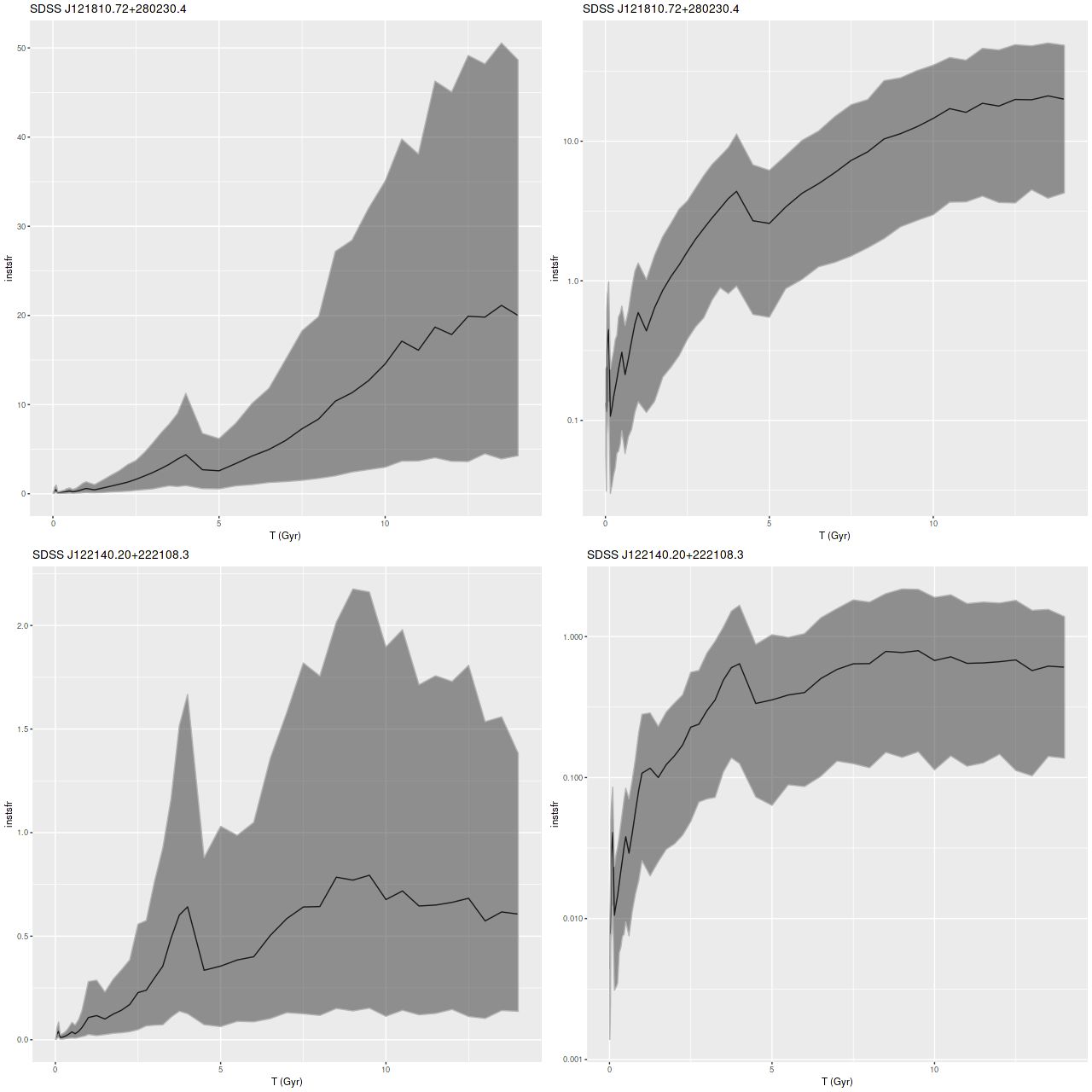
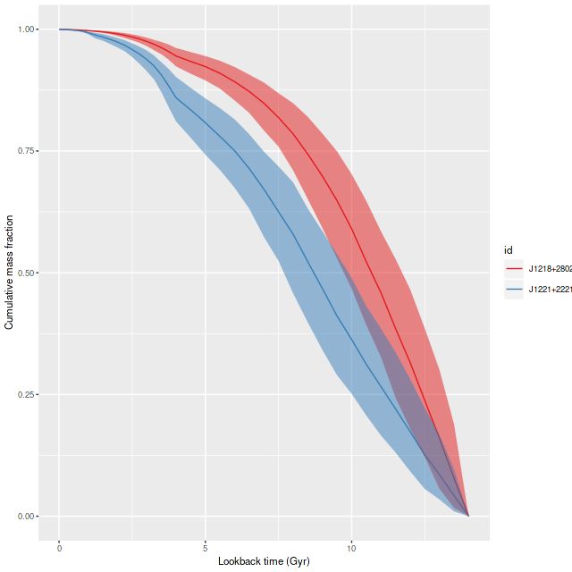
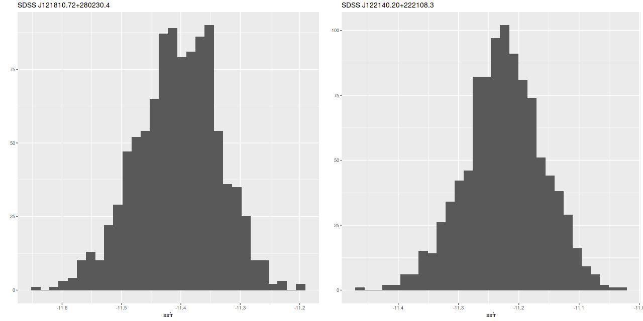
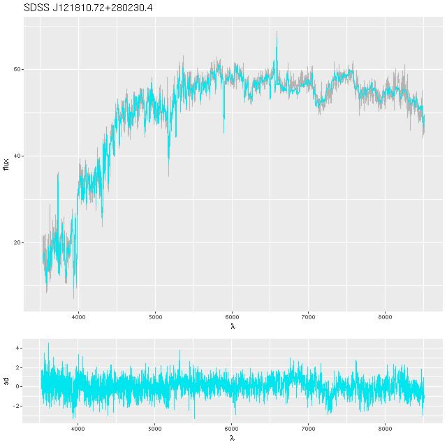
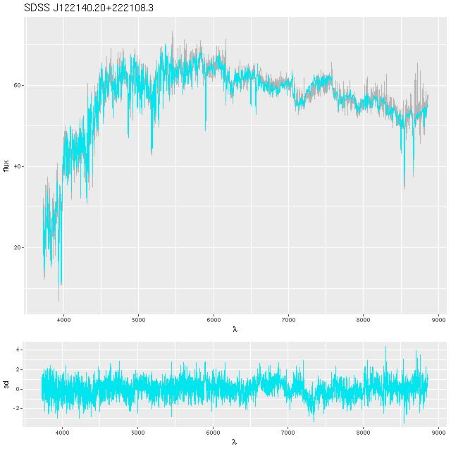
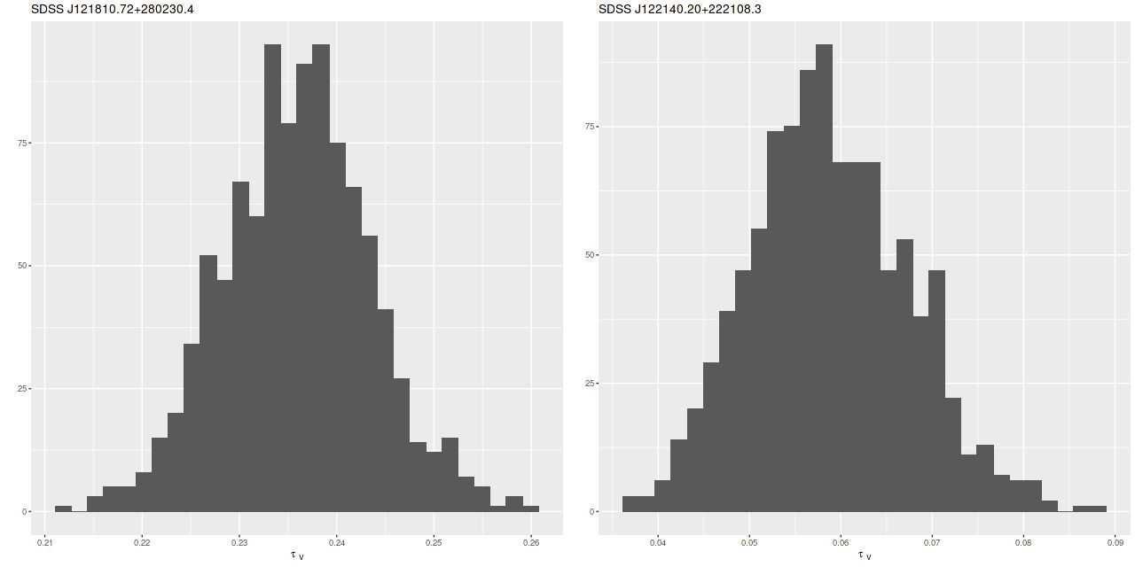
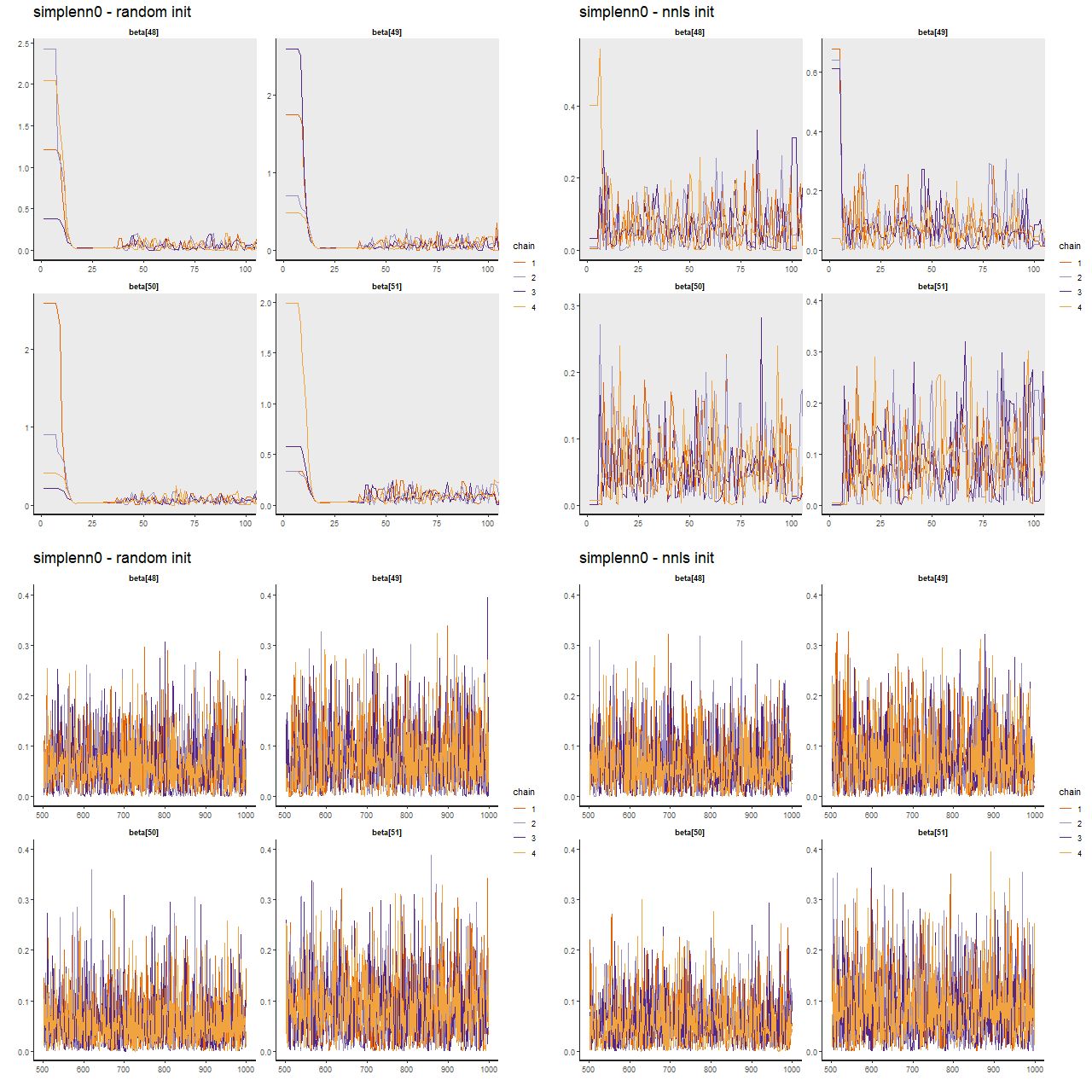
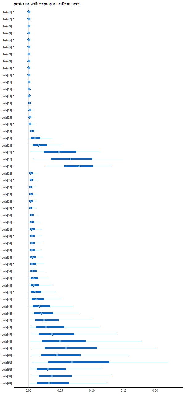
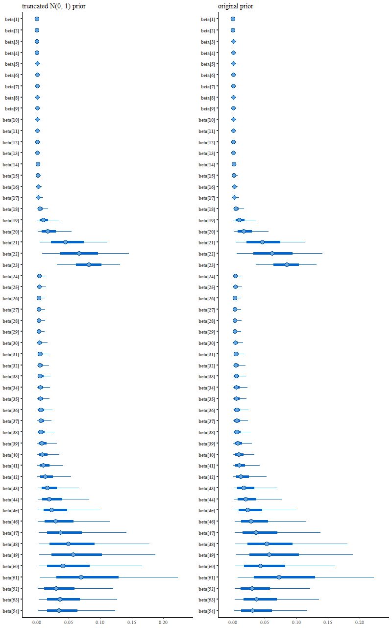
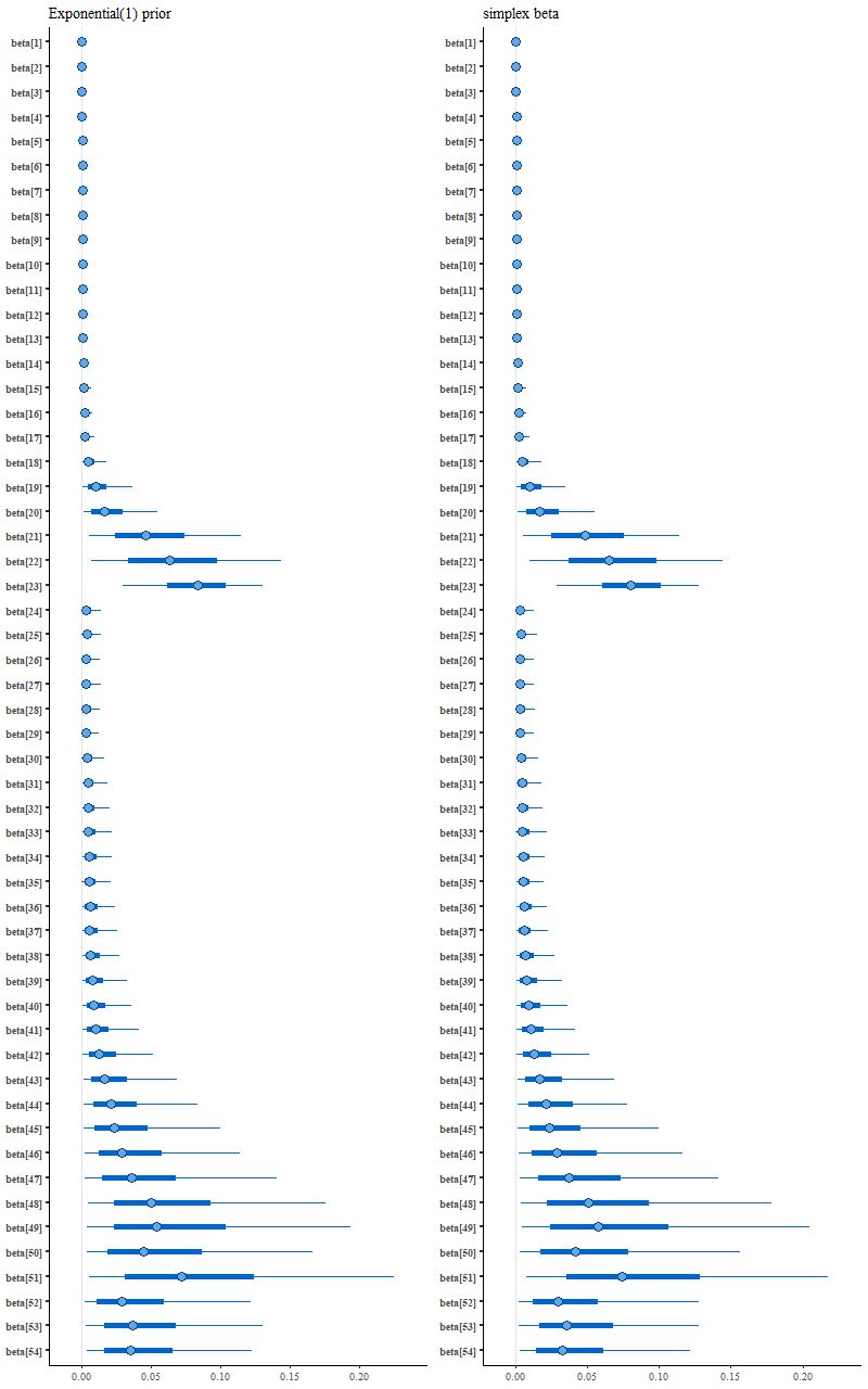
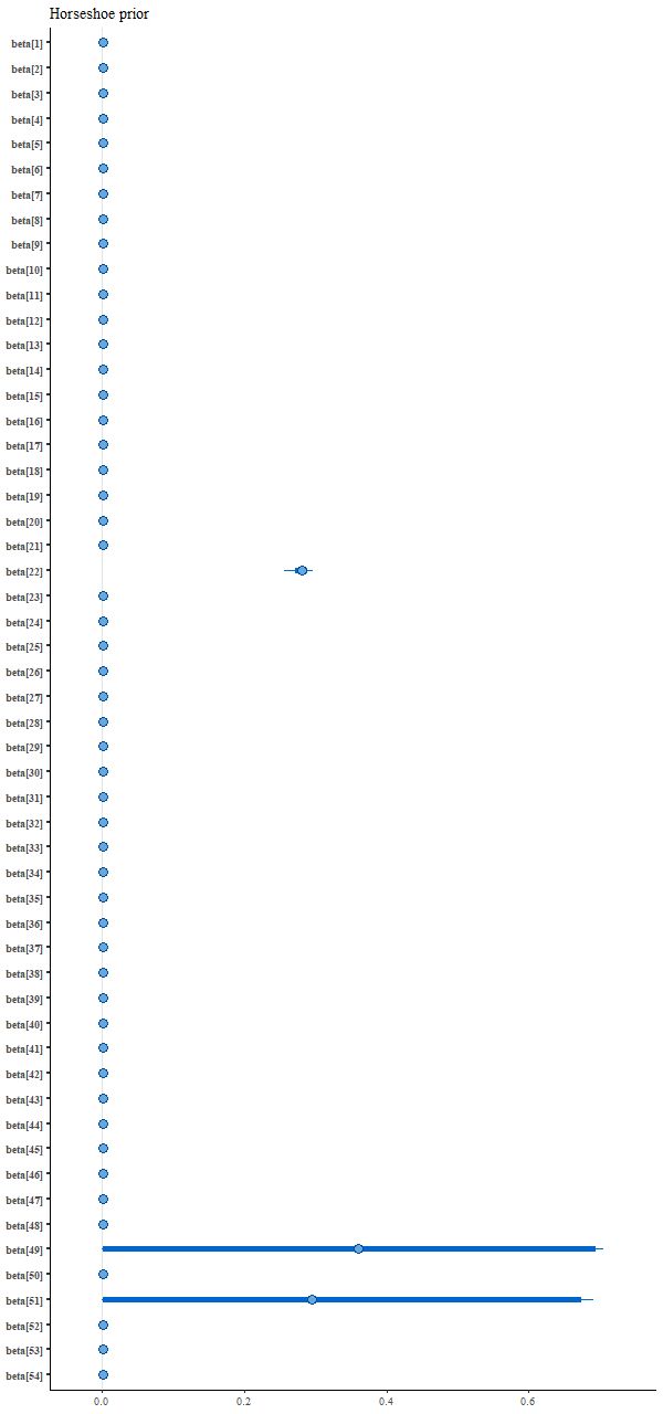
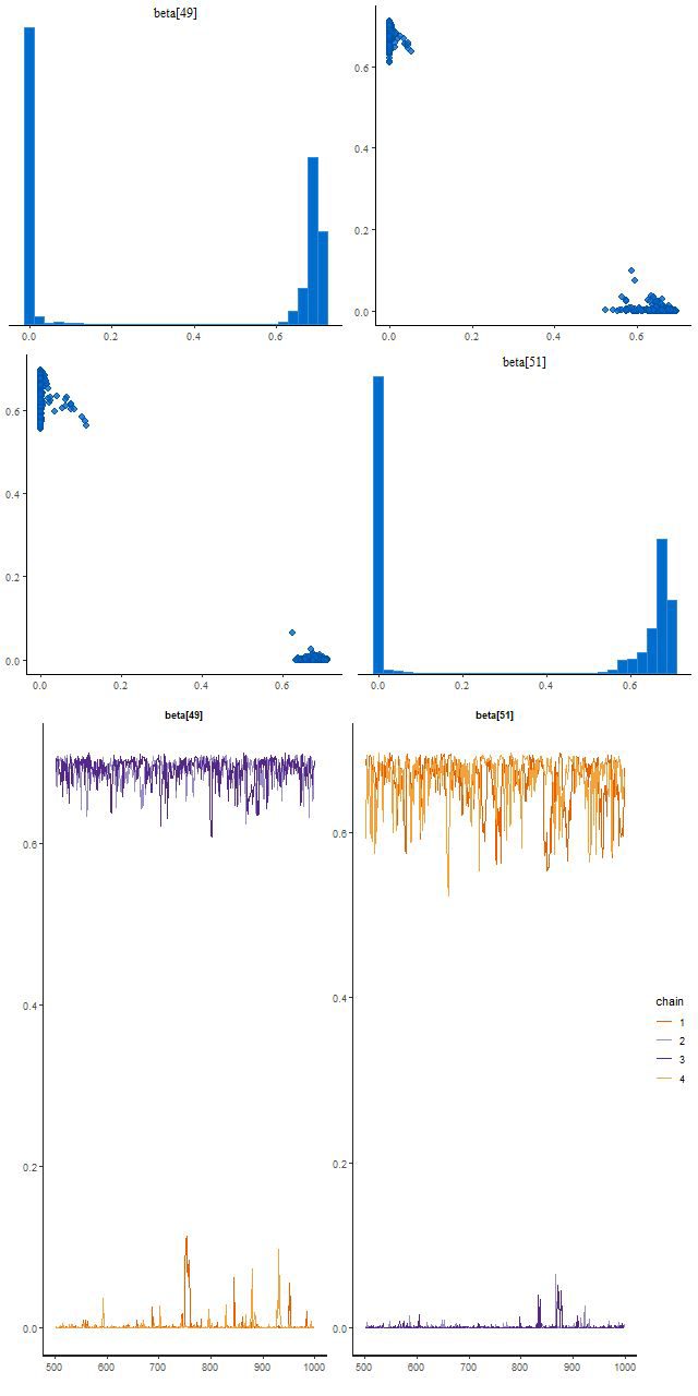
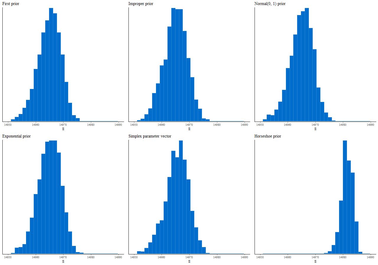
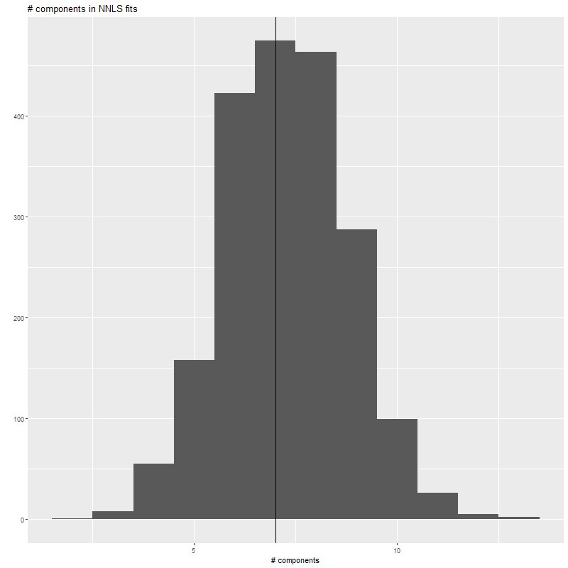
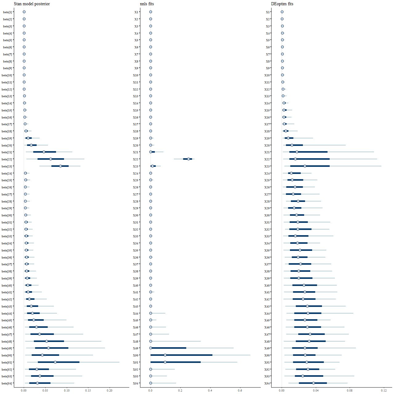
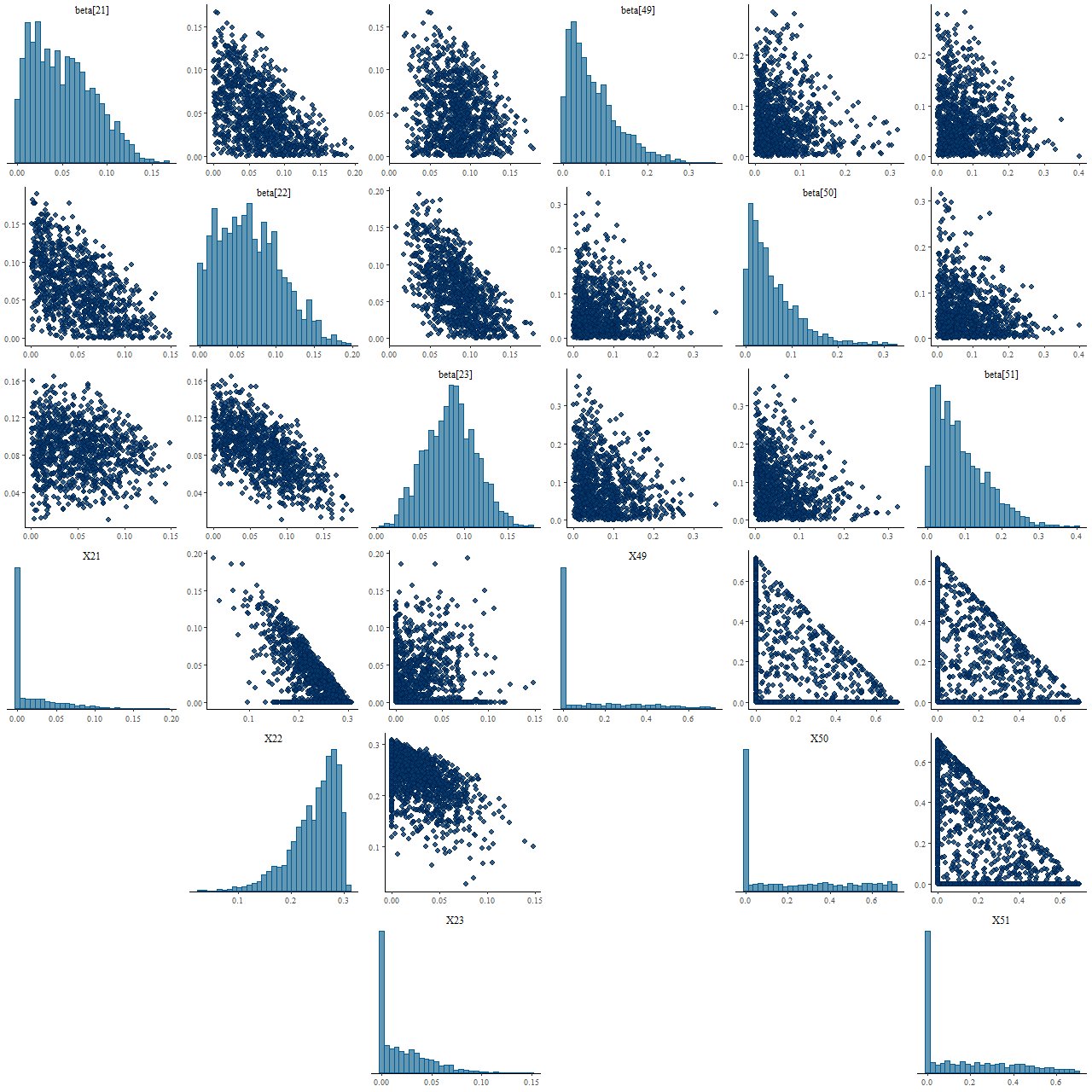
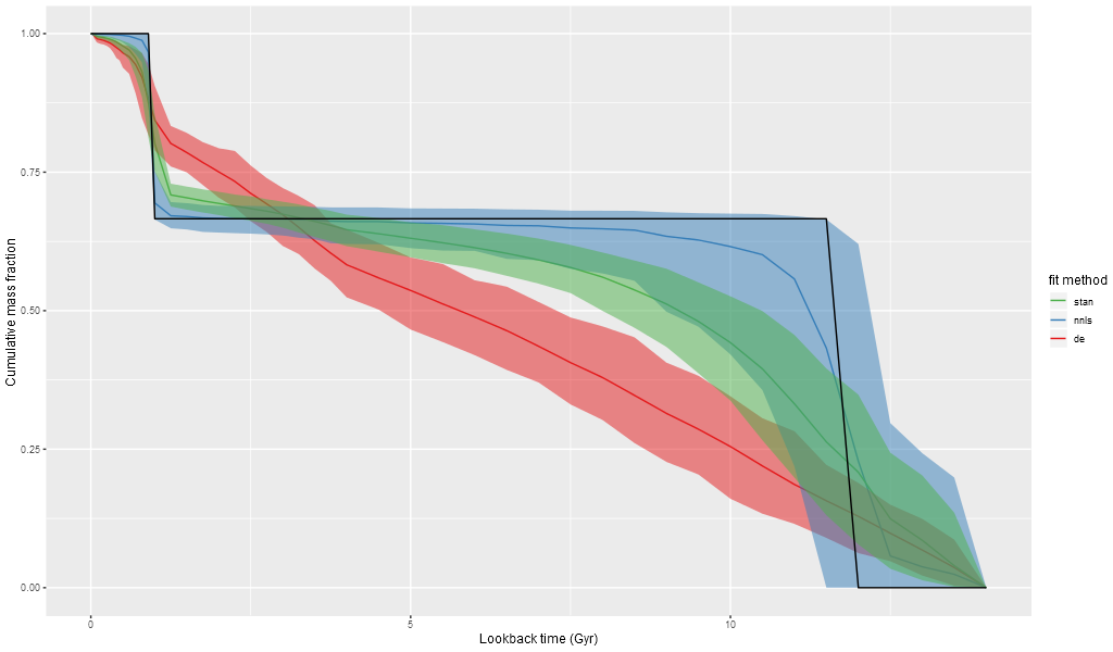
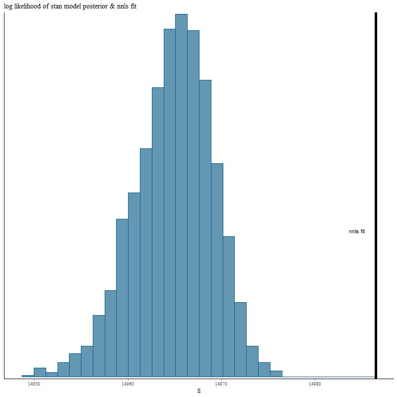
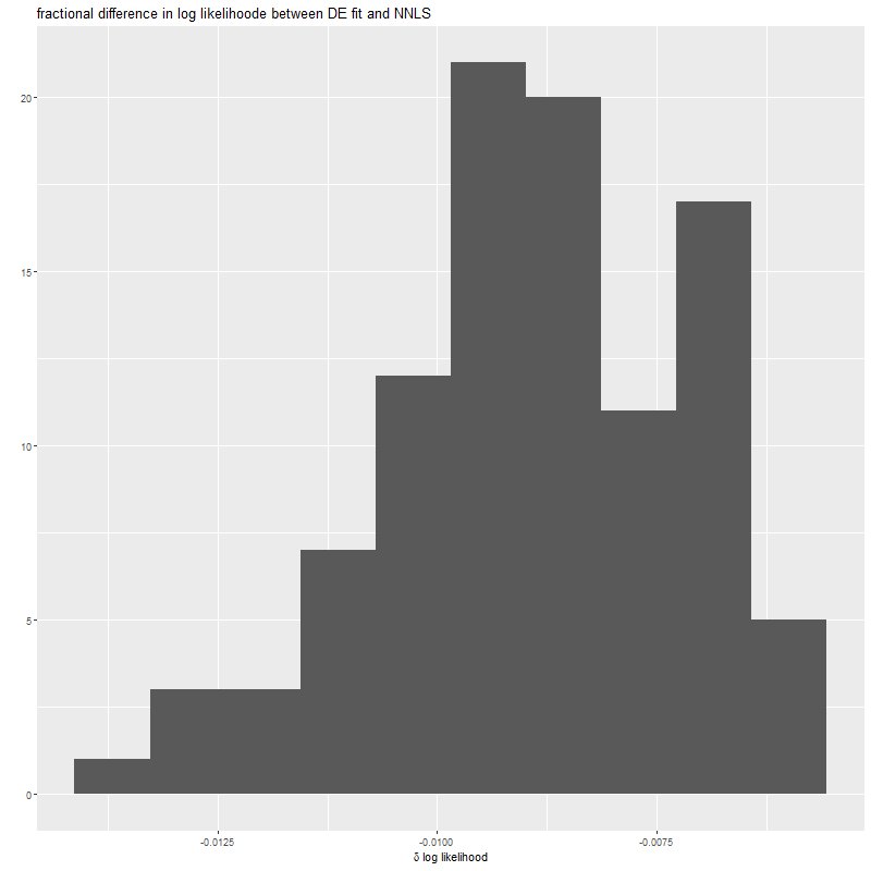
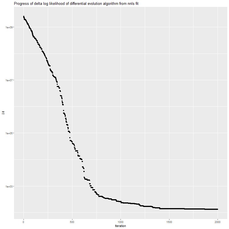
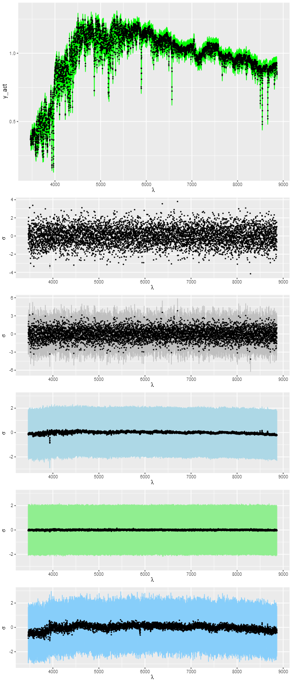
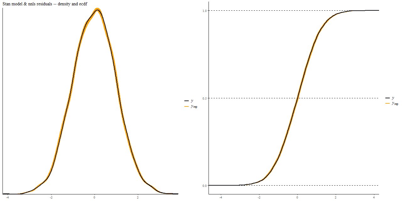
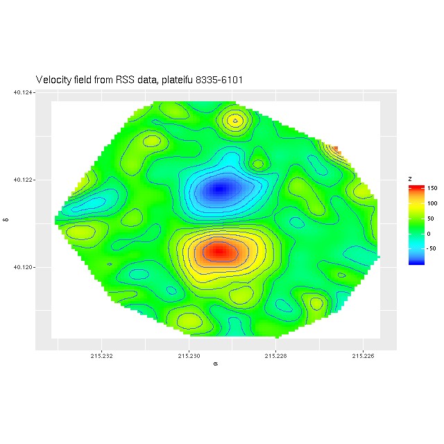 Velocity field estimated from RSS data
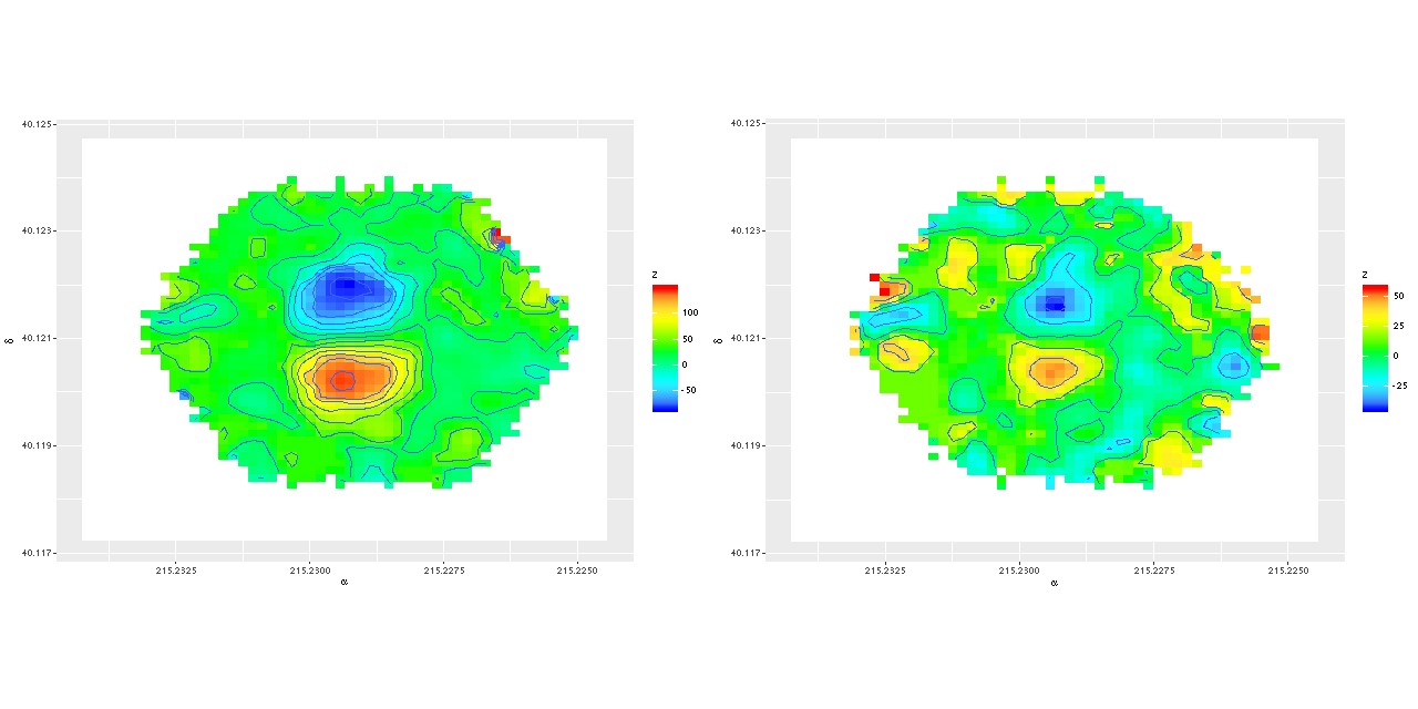 (L) Velocity field estimated for data cube
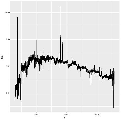 Central fiber spectrum, plateifu 8335-6101
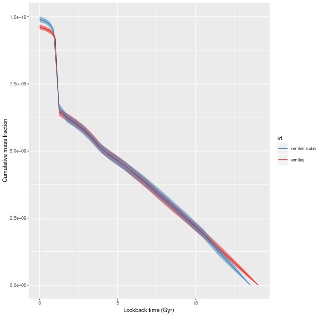 Summed model mass growth histories, emiles subset and “full” emiles
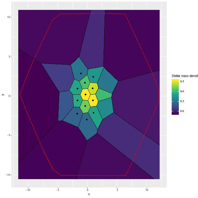 Stellar mass density for binned data, showing outlines of bins and core region
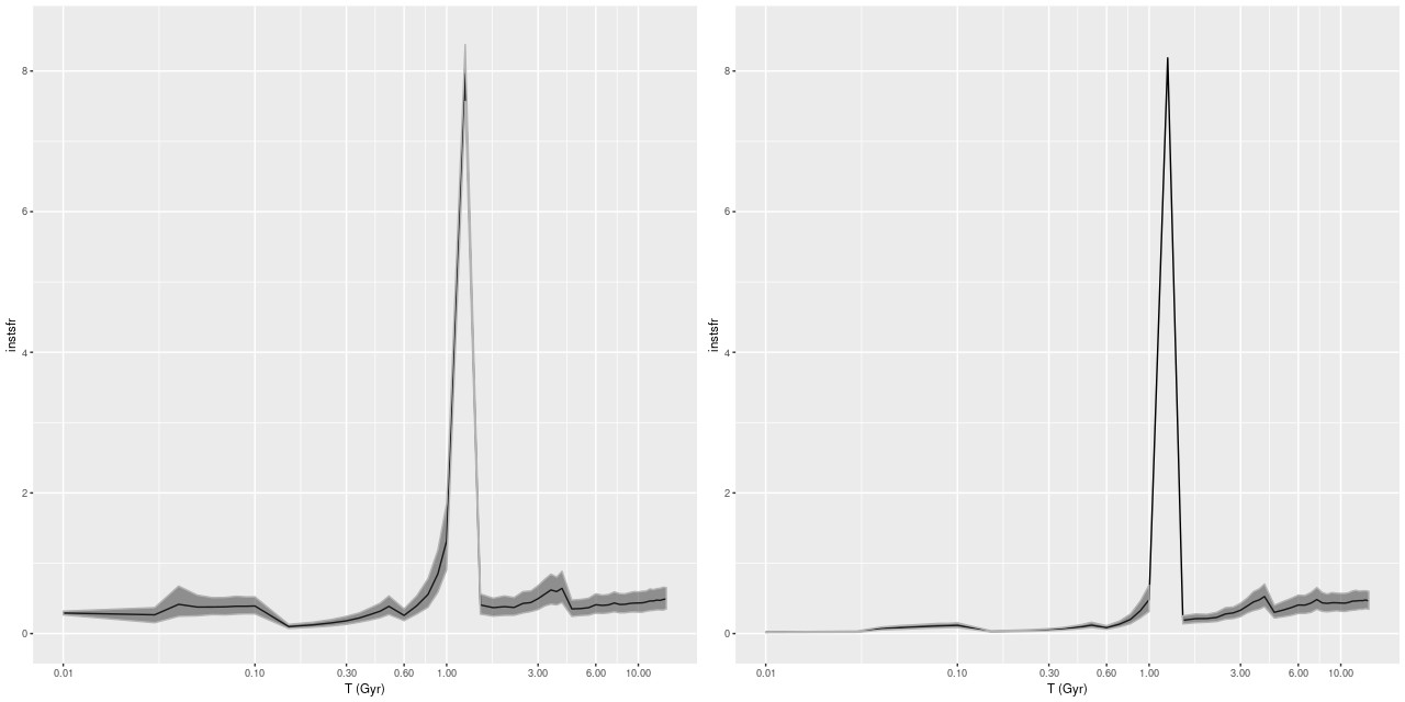 (L) Model Star formation history, inner core
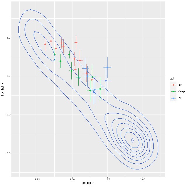 Lick HδA vs. Dn(4000)
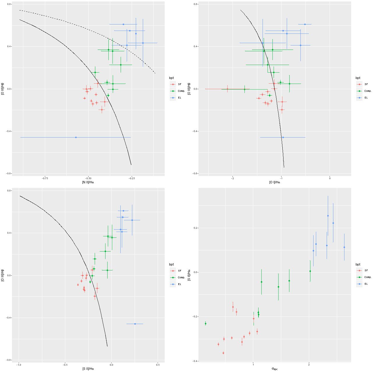 Emission line diagnostic (BPT) plots
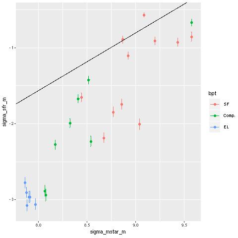 log SFR density vs. log stellar mass density
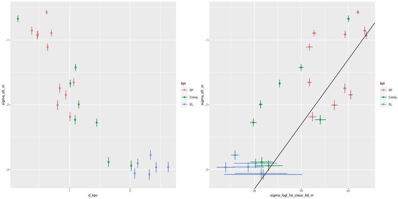 (L) log SFR density vs. radius
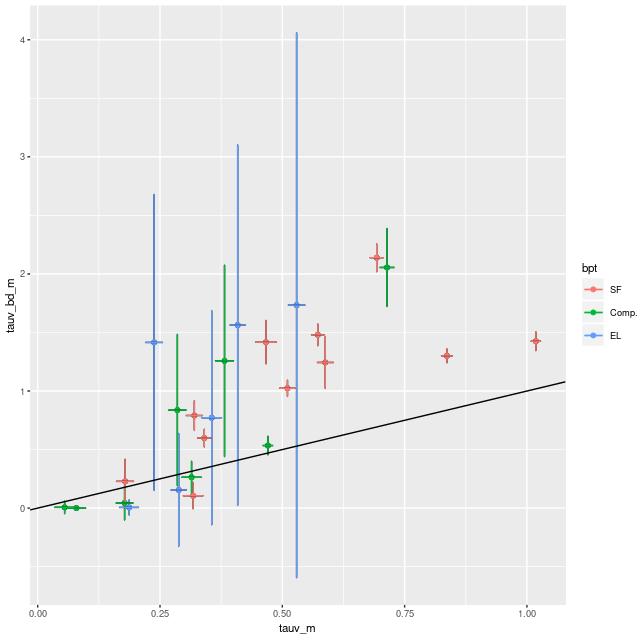 τV estimated from Balmer decrement vs SFH model estimates
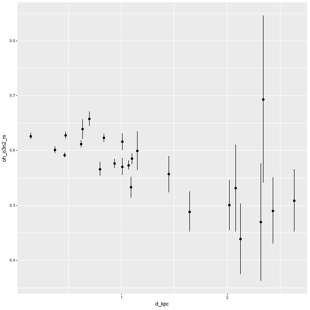 Metallicity 12+log(O/H) vs radius, estimated by O3N2 index