
I’m going to take a selective look at some of the Stan code for this model, then show some results for the RSS derived data set. The complete stan file is at <https://github.com/mlpeck/vrot_stanmodels/blob/master/vrot.stan>. By the way development is far from frozen on this little side project, so this code may change in the future or I may add new models. I’ll try to keep things properly version controlled and my github repository in sync with my local copy.
Stan programs are organized into named blocks that declare and sometimes operate on different types of variables. There are seven distinct blocks that may be present — I use 6 of them in this program. The functions block in this program just defines a function that returns the values of the polynomial representing the rotational and expansion velocities. The data block is also straightforward:
data {
int<lower=1> order; //order for polynomial representation of velocities
int<lower=1> N;
vector[N] x;
vector[N] y;
vector[N] v; //measured los velocity
vector[N] dv; //error estimate on v
real phi0;
real<lower=0.> sd_phi0;
real si0;
real<lower=0.> sd_si0;
real<lower=0.> sd_kc0;
real<lower=0.> r_norm;
real<lower=0.> v_norm;
int<lower=1> N_r; //number of points to fill in
vector[N_r] r_post;
}
The basic data inputs are the cartesian coordinates of the fiber positions as offsets from the IFU center, the measured radial velocities, and the estimated uncertainties of the velocities. I also pass the polynomial order for the velocity representations and sample size as data, along with several quantities that are used for setting priors.
The parameters block is where the model parameters are declared, that is the variables we want to make probabilistic statements about. This should be mostly self documenting given the discussion in the previous post, but I sprinkle in some C++ style comments. I will get to the length N vector parameter v_los shortly.
parameters {
  real phi;
  real<lower=0., upper=1.> sin_i;  // sine disk inclination
  real x_c;  //kinematic centers
  real y_c;
  real v_sys;     //system velocity offset (should be small)
  vector[N] v_los;  //latent "real" los velocity
  vector[order] c_rot;
  vector[order] c_exp;
  real<lower=0.> sigma_los;
}
In this program the transformed parameters block mostly performs the matrix manipulations I wrote about in the last post. These can involve both parameters and data. A few of the declarations here improve efficiency in minor but useful ways recommended in the Stan help forums by members of the development team. For example the statement real sin_phi = sin(phi); saves recalculating the sine further down.
transformed parameters {
  vector[N] xc = x - x_c;
  vector[N] yc = y - y_c;
  real sin_phi = sin(phi);
  real cos_phi = cos(phi);
  matrix[N, 2] X;
  matrix[N, 2] Xhat;
  matrix[2, 2] Rot;
  matrix[2, 2] Stretch;
  vector[N] r;
  vector[N] xhat;
  vector[N] yhat;

  X = append_col(xc, yc);
  Rot = [ [-cos_phi, -sin_phi],
          [-sin_phi, cos_phi]];
  Stretch = diag_matrix([1./sqrt(1.-sin_i^2), 1.]');
  Xhat = X * Rot * Stretch;
  xhat = Xhat[ : , 1];
  yhat = Xhat[ : , 2];
  r = sqrt(yhat .* yhat + xhat .* xhat);
}
The model block is where the log probability is defined, which is what the sampler is sampling from:
model {
  phi ~ normal(phi0, sd_phi0);
  sin_i ~ normal(si0, sd_si0);
  x_c ~ normal(0, sd_kc0/r_norm);
  y_c ~ normal(0, sd_kc0/r_norm);
  v_sys ~ normal(0, 150./v_norm);
  sigma_los ~ normal(0, 50./v_norm);
  c_rot ~ normal(0, 1000./v_norm);
  c_exp ~ normal(0, 1000./v_norm);

  v ~ normal(v_los, dv);
  v_los ~ normal(v_sys + sin_i * (
                  sump(c_rot, r, order) .* yhat + sump(c_exp, r, order) .* xhat),
                  sigma_los);
}
I try to be consistent about setting priors first in the model block and using proper priors that are more or less informative depending on what I actually know. In this case some of these are hard coded and some are passed to Stan as data and can be set by the user. I find it necessary to supply fairly informative priors for the orientation and inclination angles. For the latter it’s because of the weak identifiability of the inclination. For the former it’s to prevent mode hopping.
Stan’s developers recommend that parameters should be approximately unit scaled, and this usually entails rescaling the data. In this case we have both natural velocity and length scales. Typical peculiar velocities are on the order of no more than a few hundreds of km/sec., so I scale them to units of 100 km/sec. The MaNGA primary sample is intended to have each galaxy observed out to 1.5Reff, where Reff is the (r band) half light radius, so the maximum observed radius should typically be ∼1.5Reff. Therefore I typically divide all position measurements by that amount with the effective radius taken from nsa_elpetro_th50_r in drpcat. Other catalog values that I use as inputs to the model are nsa_elpetro_phi for the orientation angle and nsa_elpetro_ba for the cosine of the inclination. These are used as the central values of the priors and also to initialize the sampler.
Once I solved the problem of parametrizing angles the next source of pathologies I encountered was a tendency towards multimodal kinematic centers. This usually manifests as one or more chains being displaced from the others rather than mode hopping within a chain, although that can happen too. In the typical case the extra modes would place the center in an adjacent fiber to the one closest to the IFU center, but sometimes much larger jumps happen. Although I wouldn’t necessarily rule out the possibility of actual multimodality when it happens it has a severe effect on convergence diagnostics and on most other model parameters. I therefore found it necessary to place a tighter prior on the kinematic centers than I would have liked based solely on prior knowledge: the default prior puts about 95% of the prior mass within the radius of the central fiber. This could overconstrain the kinematic center in some cases, particularly low mass galaxies with weak central concentration.
A very common situation with astronomical data is to have quantities measured with error with an accompaying uncertainty estimate for each measurement. My code for estimating redshift offsets kicks out an uncertainty estimate, so this is no exception. I take a standard approach to modeling this: the unknown “true” line of sight velocity is treated as a latent variable, with the measured velocity generated from a distribution having mean equal to the latent variable and standard deviation the estimated uncertainty. In this case the distribution is assumed to be Gaussian. The latent variable is then treated as the response variable in the model. Since I had no particular expectations about what the residuals from the model should look like I fell back on the statistician’s standard assumption that they are independent and identically distributed gaussians with standard deviation to be estimated as part of the model.
Having a latent parameter for every measurement seems extravagant, but in fact it causes no issues at all except for a slight performance penalty. With the distributional assumptions I made the latent variables can be marginalized out and posteriors for the remaining parameters will be the same within typical Monte Carlo variability. The main performance difference seems to arise from slower adaptation in the latent variables version.
Finally, some results from the observation with plateifu 8942-12702 (mangaid 1-218280). First, the measured velocity field and the posterior mean model. The observations came from the same data shown in the previous post interpolated onto a finer grid.
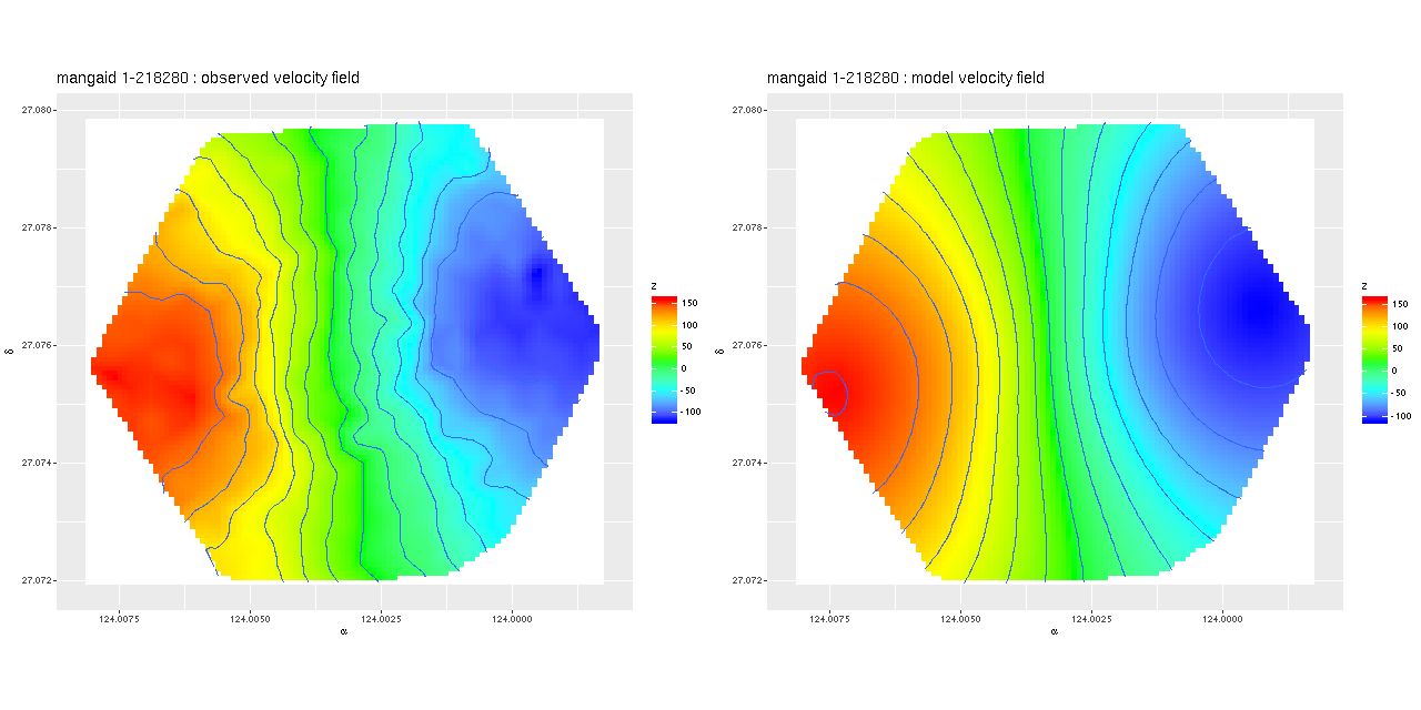
The model seems not too bad except for missing some high spatial frequency details. The residuals may be revealing (again this is the posterior mean difference between observations and model):
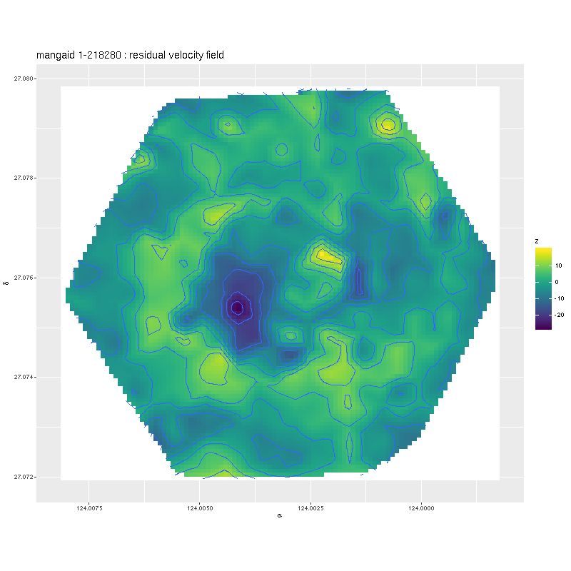
There is a strong hint of structure here, with a ridge of positive residuals that appears to follow the inner spiral arms at least part of the way around. There are also two regions of larger than normal residuals on opposite sides of the nucleus and with opposite signs. In this case they appear to be at or near the ends of the bar. This is a common feature of these maps — I will show another example or two later.
Next are the joint posterior distributions of \(v_{rot}\) with radius r and \(v_{exp}\) with r. Error bars are 95% credible intervals.
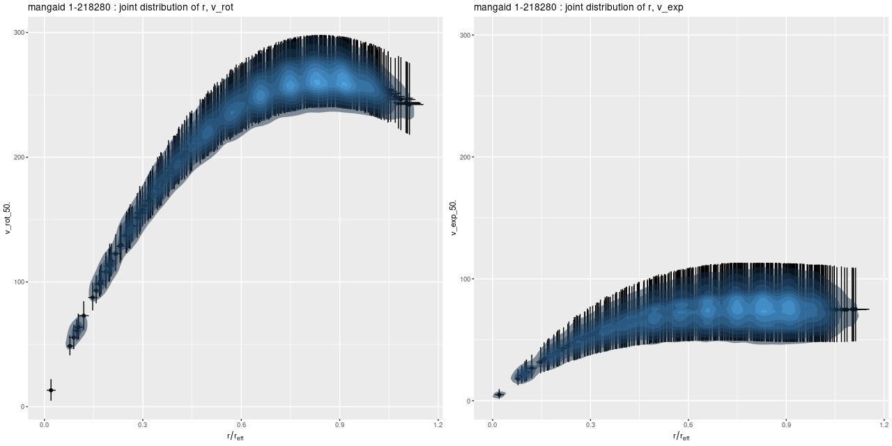
The rotation curve seems not unrealistic given the limited expressiveness of the polynomial model. The initial rise is slow compared to typical examples in the literature, but this is probably attributable to the limited spatial resolution of the data. The peak value is completely reasonable for a fairly massive spiral. The expansion velocity on the other hand is surprising. It should be small, but it’s not especially so. Nowhere do the error bars include 0.
There are a number of graphical tools that are useful for assessing MCMC model performance. Here are some pairs plots of the main model parameters:
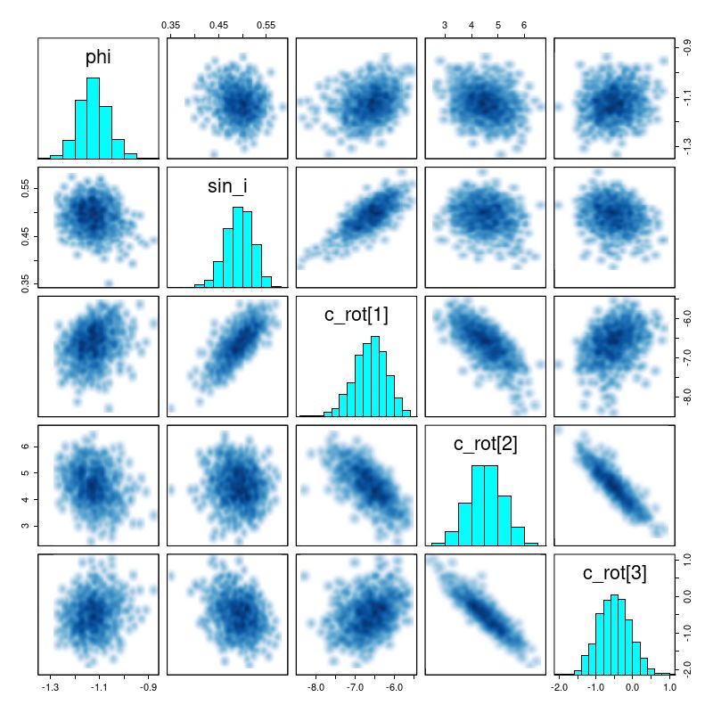
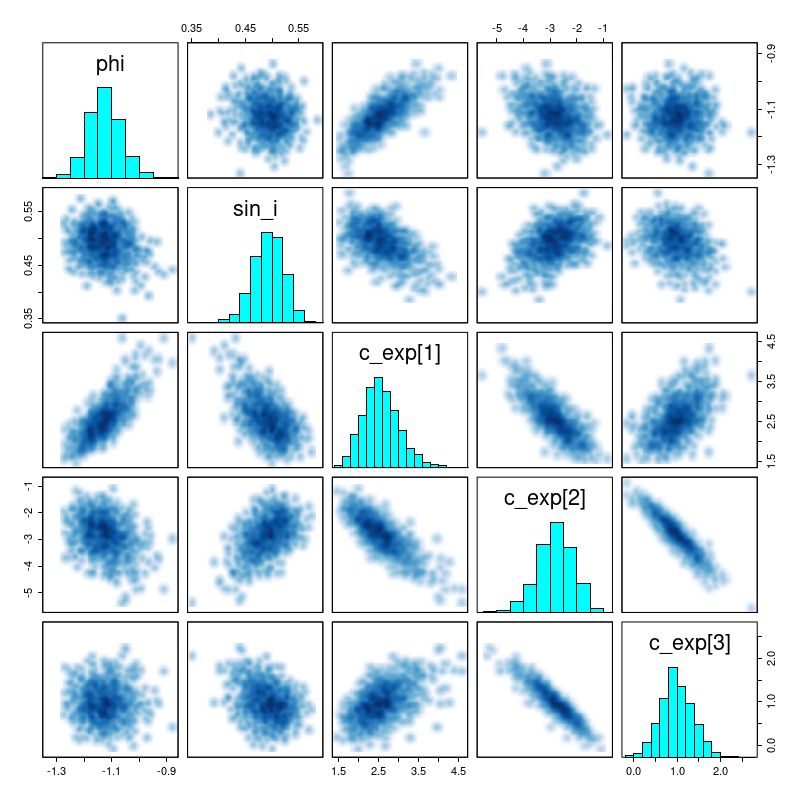
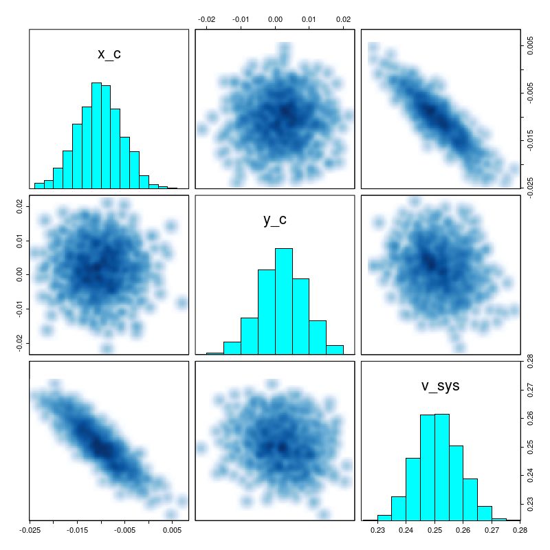
There are several significant correlations here, none of which are really surprising. The polynomial coefficients are strongly correlated. The inclination angle is strongly correlated with rotation velocity and slightly less, but still significantly correlated with expansion velocity. The orientation angle is slightly correlated with rotation velocity but strongly correlated with expansion. The estimated system velocity is strongly correlated with the x position of the kinematic center but not y — this is because the rotation axis is nearly vertical in this case. The relatively high value of v_sys (posterior mean of 25 km/sec) is a bit of a surprise since the SDSS spectrum appeared to be well centered on the nucleus and with an accurate redshift measurement. Nevertheless the value appears to be robust.
Stan is quite aggressive with warnings about convergence issues, and it reported none for this model run. No graphical or quantitative diagnostics indicated any problems. Nevertheless there are several indicators of possible model misspecification.
- Signs of structure in residual maps are interesting because they indicate perturbations of the velocity field as small as ∼10 km/sec by spiral structure or bars may be detectable. But it also indicates the assumption of iid residuals is false.
- It’s hard to tell from visual inspection if the symmetrically disposed velocity residuals near the nucleus are due to rotating rings of material or streaming motions, but in any case a low order polynomial can’t be fit to them. I will show more dramatic examples of this in a future post.
- Large scale expansion (or contraction) shouldn’t be seen in a disk galaxy, but the estimated expansion velocity is rather high in this case. Perturbations by the rather prominent bar would indicate that a model with a \(2 \theta\) angular dependence should be explored.
Next up, a possible partial solution.