One simple way to quantify the burstiness of star formation is just to estimate the average star formation rate over large time intervals divided by the average SFR over cosmic time. Of particular interest is the time interval between ~100 Myr and ~1 Gyr since this is roughly the time interval that a post-starburst galaxy is recognizable as such.
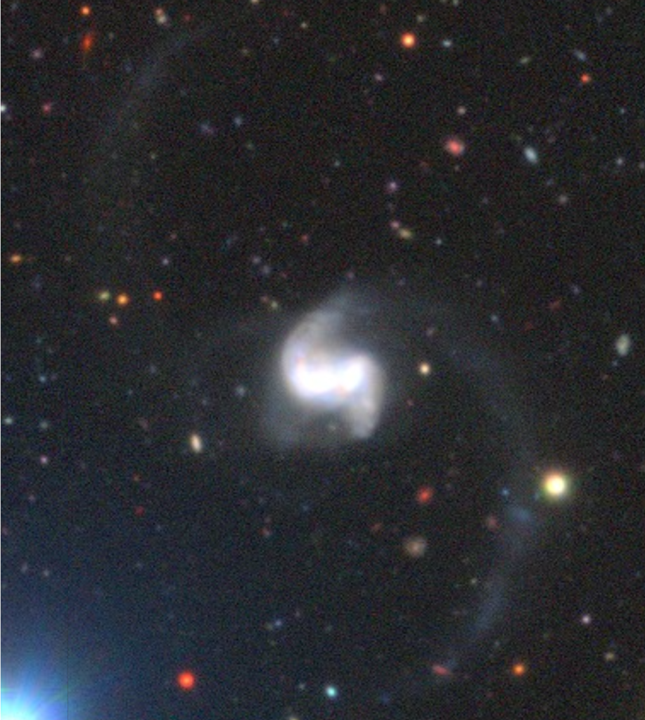
Partly because it happens to still be in my active workspace and partly because it’s really interesting I’m going to take another look at SDSS J095343.89-000524.7 (MaNGA mangaid 1-897). This was in the post-starburst ancillary sample, selected from the catalog by Pattarakijwanich et al.
This image from the Subaru HSC-SSP survey1retrieved as a screenshot from the Legacy Survey sky browser. is much deeper than SDSS imaging and clearly shows extended tidal tails and debris, suggesting that these galaxies have been interacting for some time.
SDSS J095343.89-000524.7 (observed as mangaid 1-897).
Image screenshot from Subaru HSC survey.
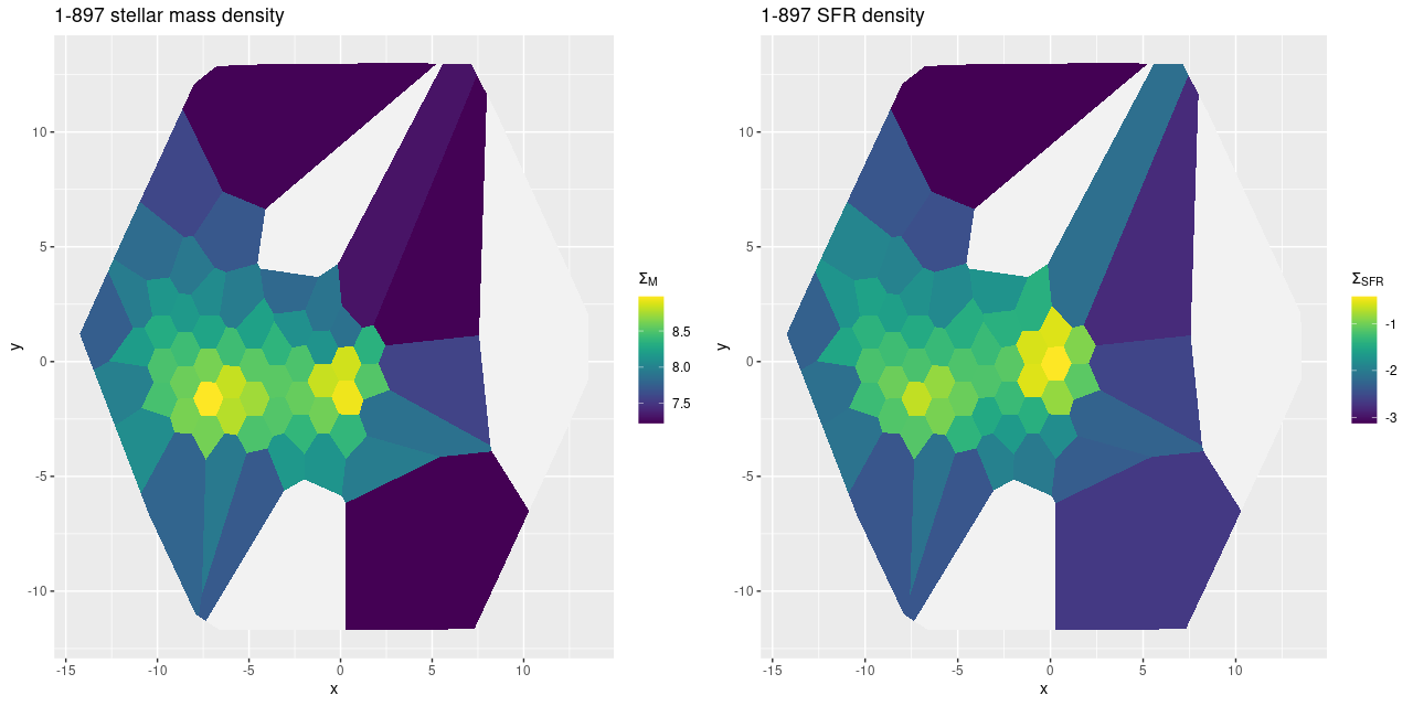
Moving on to various properties derived from the MaNGA spectroscopy and my SFH models with, still, EMILES based SSP models. First here are maps of stellar mass density and 100 Myr averaged star formation rate density. Note that I rebinned the spectra from two posts ago to try to capture more of the tidal tails while excluding the truly blank regions of sky. There are two clear peaks in the stellar mass density separated by a projected distance of about 11 kpc. The central stellar mass densities are nearly the same at about 108.95 M☉/kpc2 . Interestingly enough the bright white peak in surface brightness appears not to coincide with the western peak in stellar mass density, but is offset by a small amount to the north.
Note also that the highest recent star formation is offset to the north of the apparent western nucleus. I’ll look at that in more detail below.
MaNGA plateifu 10843-9101 (mangaid 1-897). Maps of stellar mass density and star formation rate density.
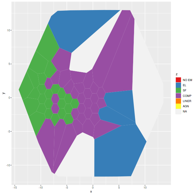
The ionized gas properties are rather different in the two galaxies. Below are BPT classifications using, as usual for me, just the [O III]/Hβ vs. [N II]/Hα diagnostics and Kauffmann’s classification scheme. Emission line fluxes are generally stronger in the eastern galaxy with mostly star forming line ratios. Note two spectra with “composite” line ratios are near the eastern nucleus and might therefore actually be due to a mix of stellar and AGN ionization.
MaNGA plateifu 10843-9101 (mangaid 1-897). BPT classifications from [O III]/Hβ vs. [N II]/Hα diagnostics
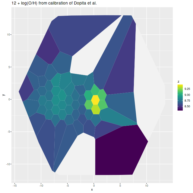
I calculate a few “strong line” gas metallicity estimates from standard literature sources. The one that seems to produce the most consistent estimates is the calibration of Dopita et al. (2016) based on the ratios of [N II 6548]/[S II 6717, 6731] and [N II]/Hα. The eastern galaxy shows a fairly smooth radial gradient while the west is considerably metal enriched in the region with the strongest starburst. The highest metallicity is right at the center of the IFU at the position of the bright white source.
MaNGA mangaid 1-897 (plateifu 10843-9101). Gas phase metallicity 12 + log(O/H) from strong line calibration of Dopita et al. (2016).
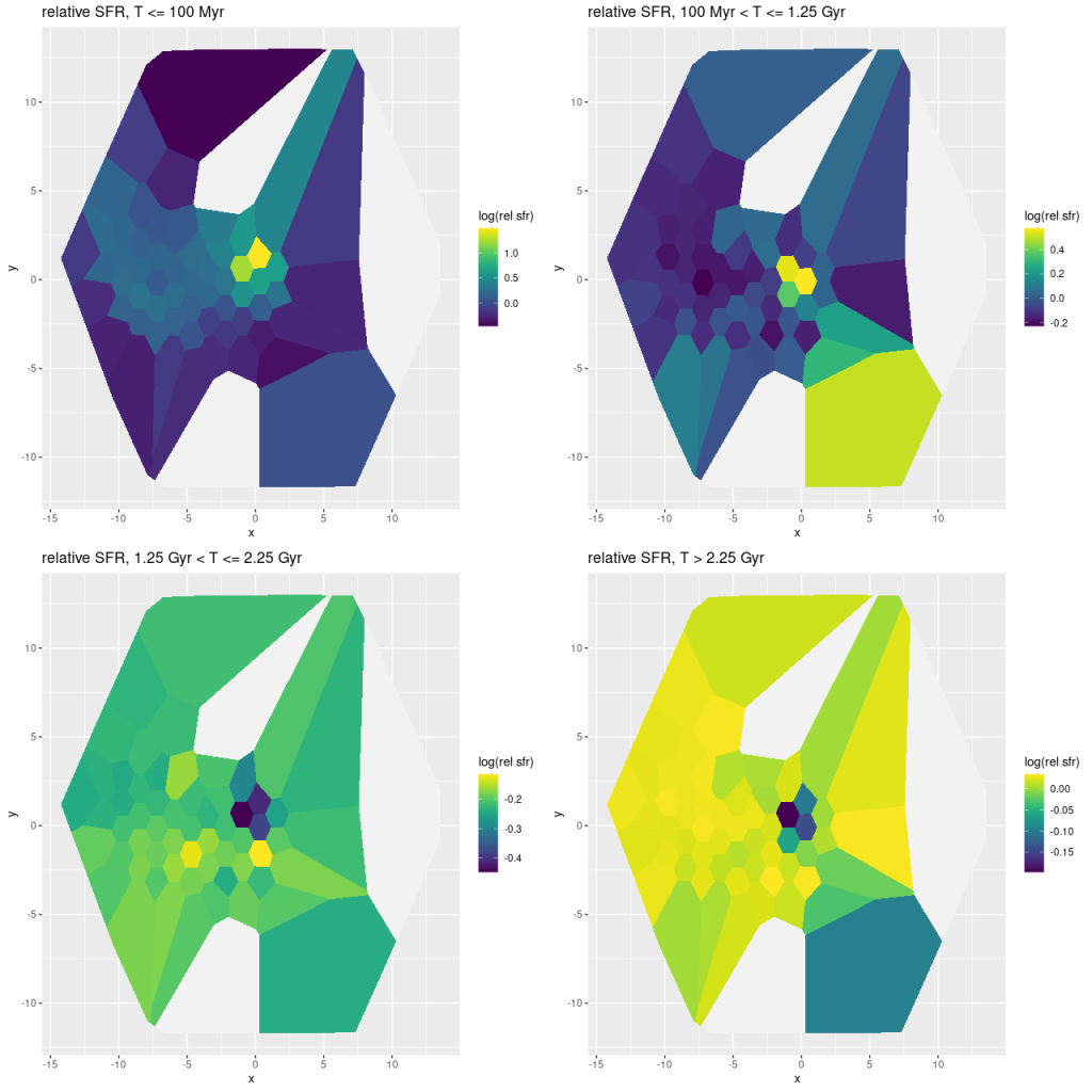
Let’s return to the idea I had at the top of the post to look at star formation rates in broad time intervals relative to the mean star formation rate over cosmic time. For this exploratory exercise I used just 4 bins with upper age limits of 0.1, 1.25, 2.25, and (nominally) 14 Gyr. There seems no point being too fastidious about calculating the bin widths: I just used the difference in nominal ages between the endpoints. I did take into account the lookback time to the galaxy, which for this one is about 1 Gyr (z = 0.083), so the final bin has a calculated width of 10.5Gyr. I chose to make the 3rd, intermediate age bin a rather short 1 Gyr wide to look for aging starbursts that might be missed using the typical selection criterion of strong Balmer absorption. In this case there’s no evidence of that: both galaxies seem to have had uneventful histories up until ~1 Gyr ago.
The top row of the plot below is the most interesting: there appear to have been two major bursts of recent star formation, both highly localized to the central region of the western galaxy. If the model estimate of the location of the peak stellar mass density is correct the fiber with the largest star formation excess in the 100 Myr – 1.25Gyr interval is offset just to the north and coincident with the IFU center. The more recent burst is also offset from the older one. There is a hint of recent accelerated star formation over most of both galaxies.
MaNGA plateifu 10843-9101 (mangaid 1-897). Maps of relative average SFR over the designated time intervals.
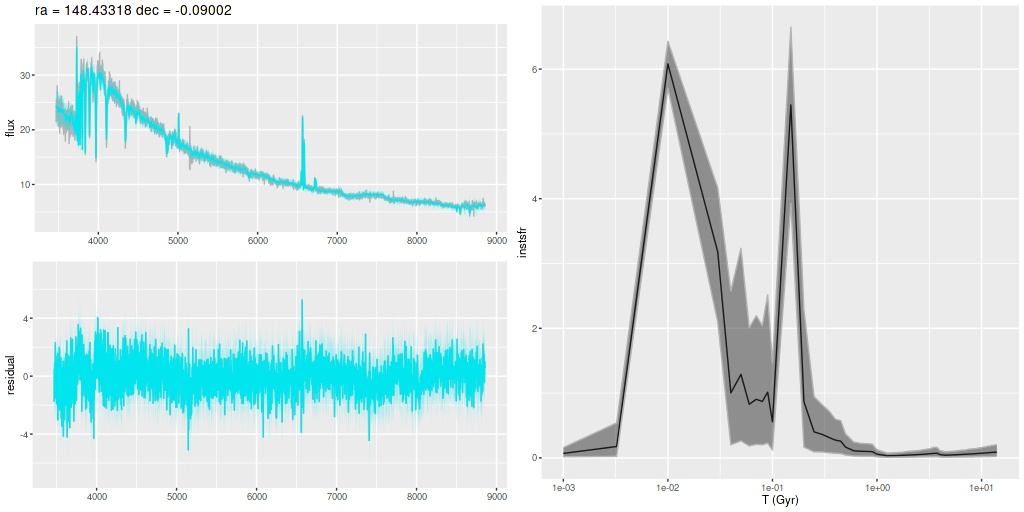
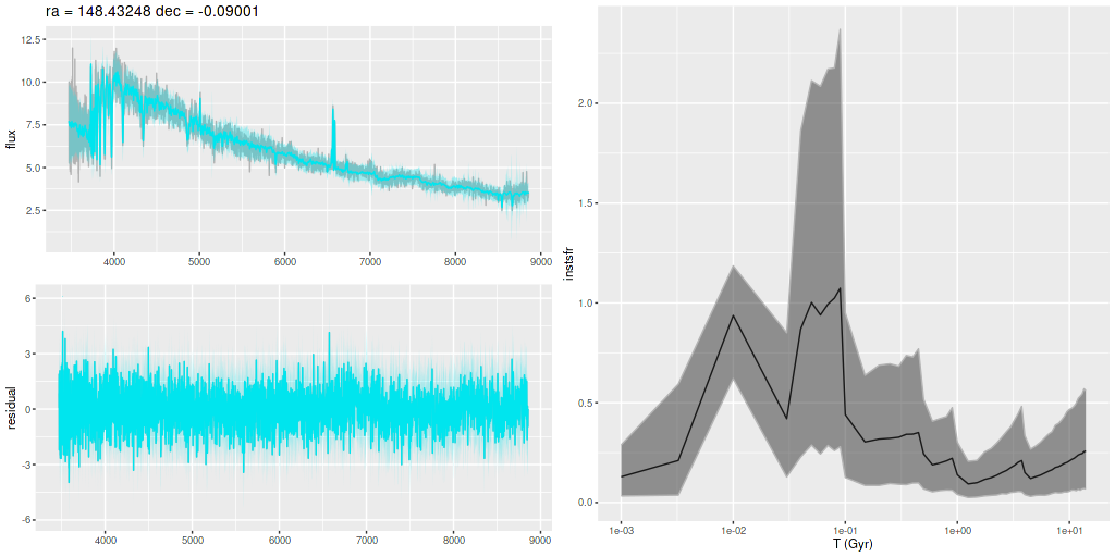
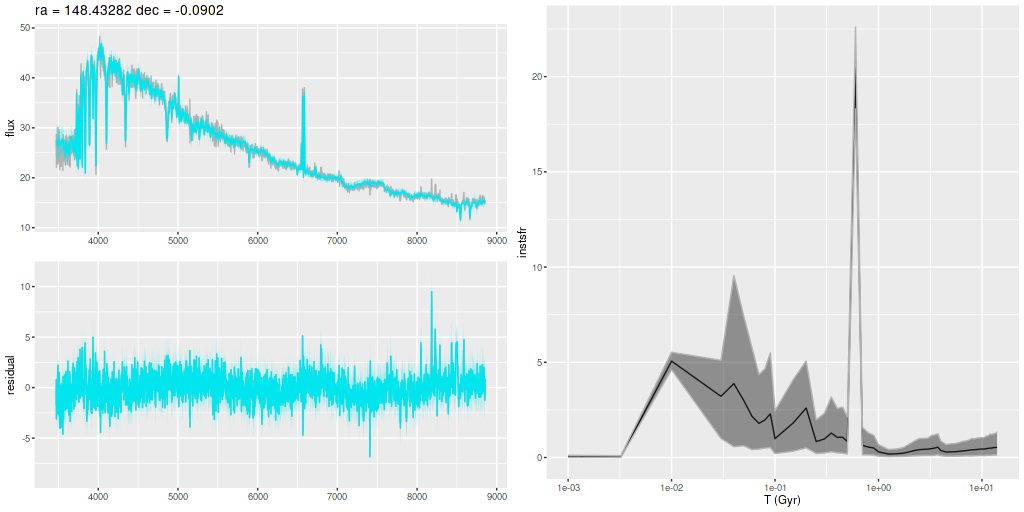
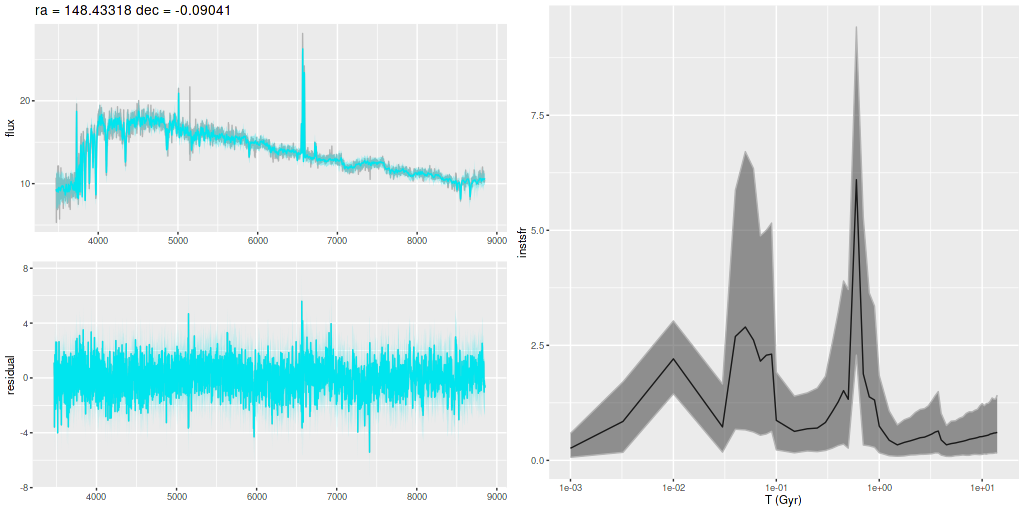
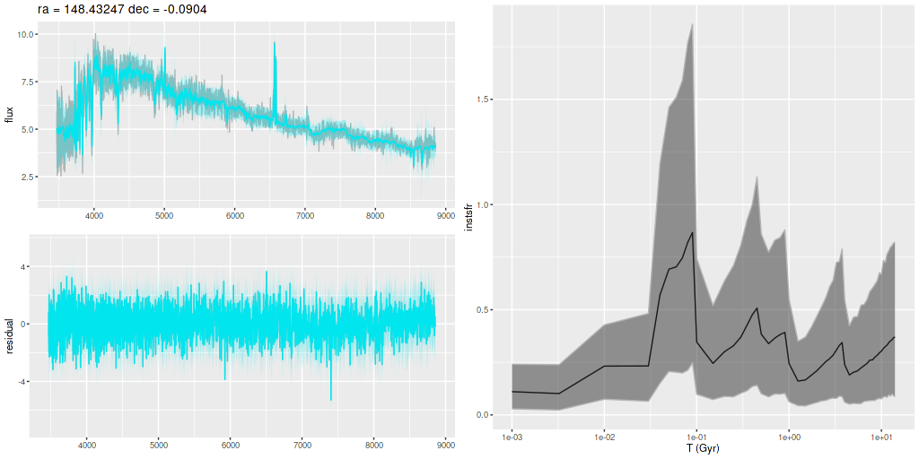
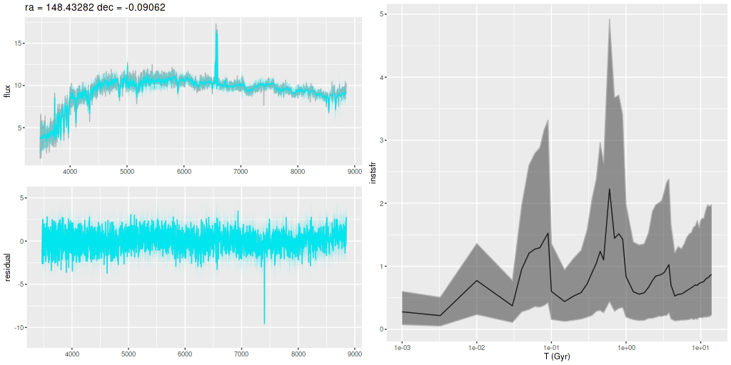
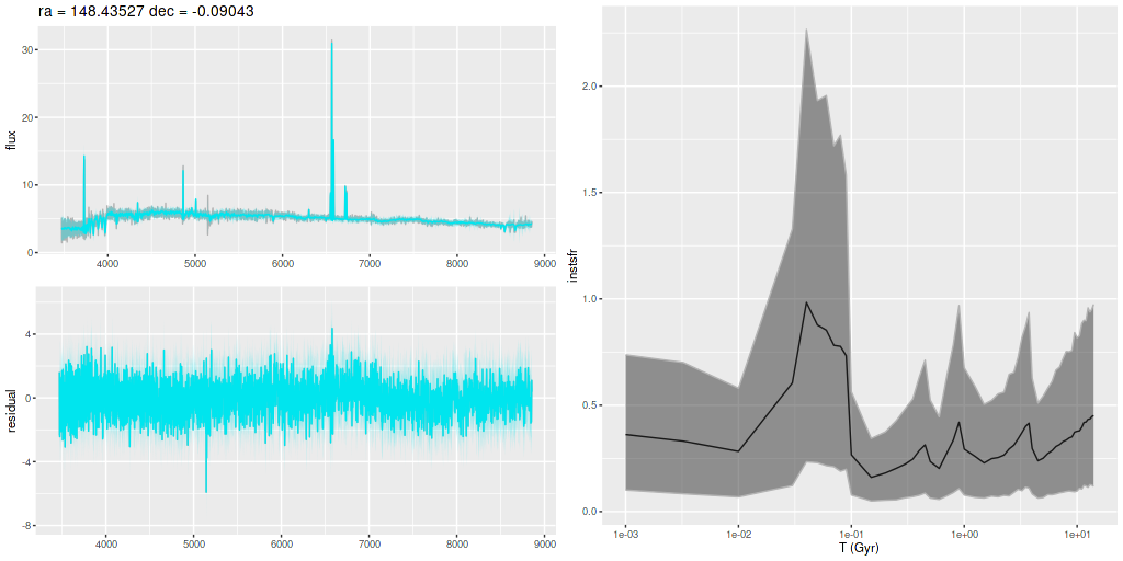
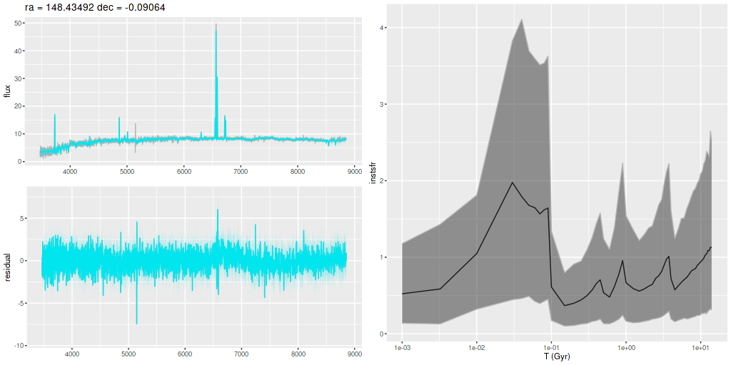
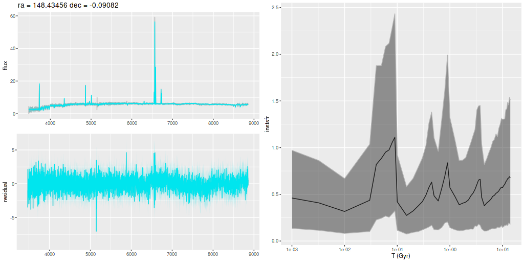
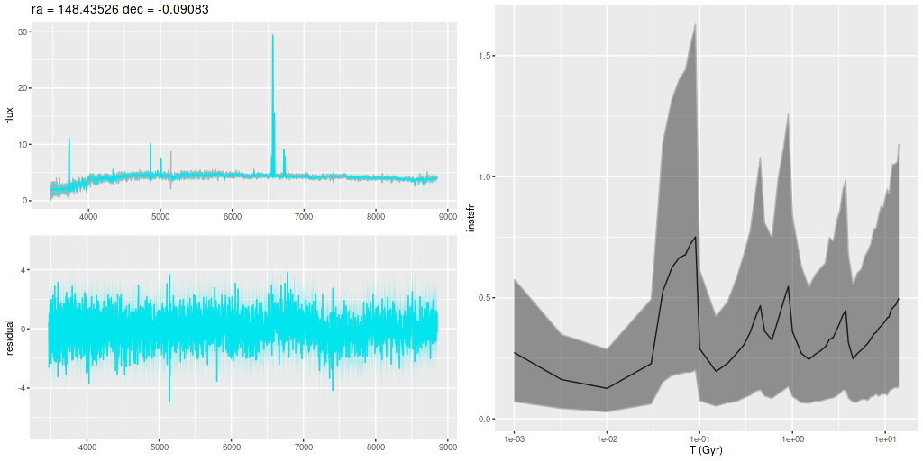
For the rest of this post I plot model fits to the spectra and star formation histories for the fibers surrounding the two nuclei. These are ordered approximately from north to south and west to east. For reference the IFU center is at (ra, dec) = (148.43291, -0.09018). The model has the peak stellar mass density in the western system at (ra, dec) = (148.4328, -0.09062). The eastern galaxy’s nucleus is at (ra, dec) = (148.4349, -0.09064).
Note below that the plots have different vertical scales. The horizontal scales are the same for both spectra and star formation histories, but at least one SFH plot is slightly misaligned.
Central region – western galaxy
MaNGA mangaid 1-897 — central region of western galaxy – spectra with fits and model star formation histories
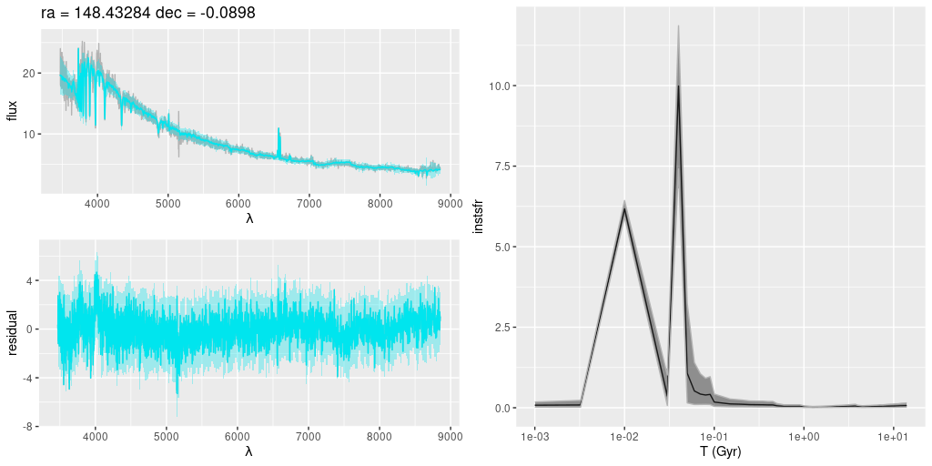
Central region – eastern galaxy
MaNGA mangaid 1-897 — central region of eastern galaxy – spectra with fits and model star formation histories
In an earller post I mentioned a MaNGA related paper by Cheng et al. who found nearly 500 systems with post-starburst characteristics that fell in 3 broad categories: centrally concentrated PSB regions, ring-like, and irregularly located. Clearly any galaxy that was selected based on SDSS spectroscopy that’s not a false positive will have a central PSB region, although that of course doesn’t preclude extended post-starburst conditions. This particular galaxy appears to have a remarkably compact post-starburst region.
When time permits again I plan to look at the remaining 40 galaxies in this sample. Unfortunately the larger sample of Cheng et al. appears to have no published catalog.
I haven’t given up on this topic. Just a longer than expected break.
I found two other catalogs of candidate PSBs selected from SDSS spectroscopy. First are the “SPOGs” (Shocked POst-starburst Galaxies” of Alatalo et al. (2016), with the catalog retrieved from VizieR at J/ApJS/224/38/table2. These were selected to have strong emission lines with ratios consistent with shocks as the ionizing mechanism, while also having strong Balmer absorption indicating the presence of a large intermediate age stellar light contribution.
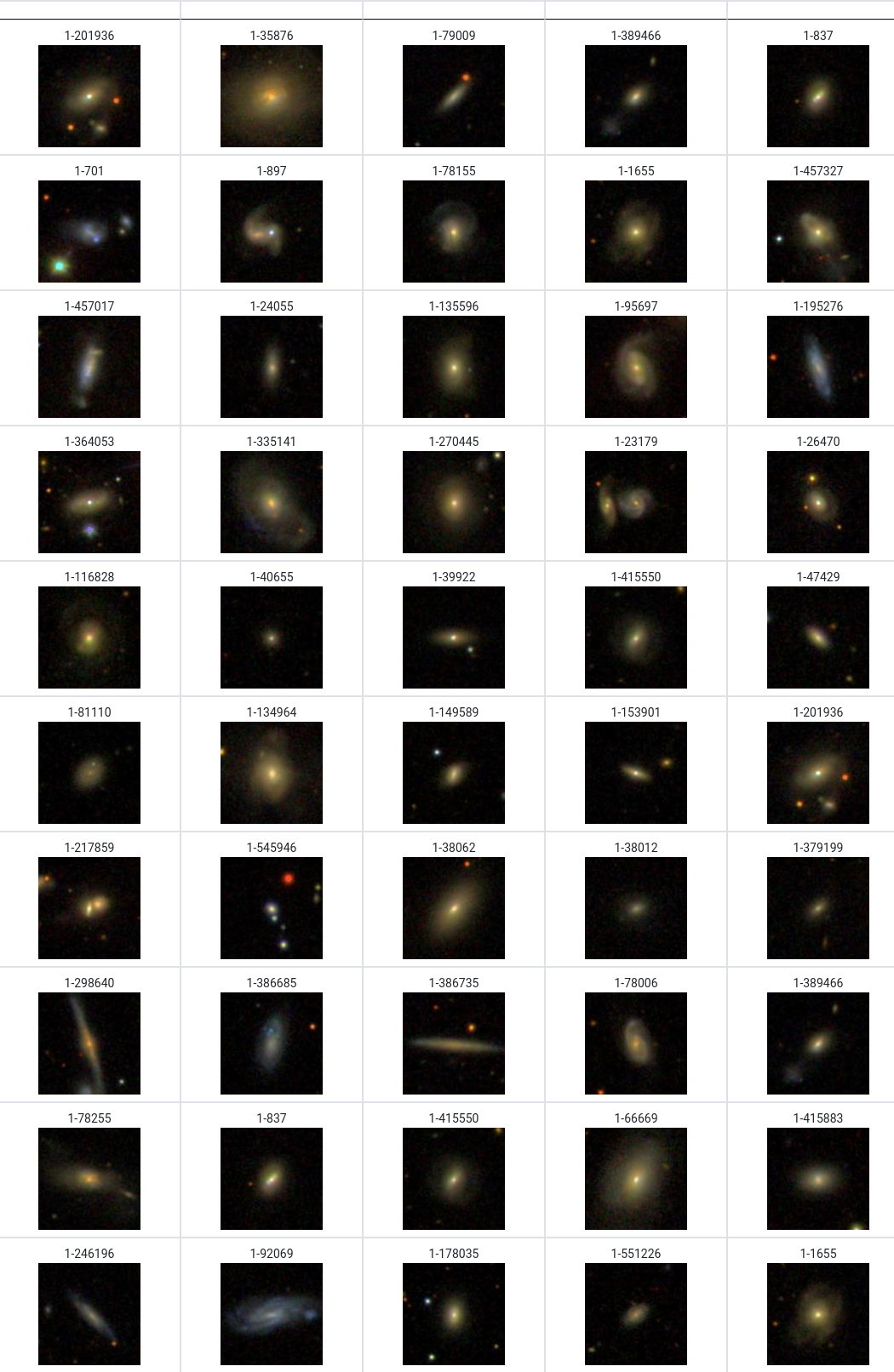
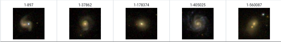
The second was the sample of Pattarakijwanich et al. (2016) retrieved from J/ApJ/833/19/table3. This work used more traditional post-starburst selection criteria although somewhat more relaxed than for example Goto. Together these added 19 galaxies to the sample — 14 SPOGs and 5 from Patta… Together these, along with the Melnick and dePropris sample added about 1000 binned spectra to the sample.
I’m not going to say much about them for now. SDSS thumbnails are below. One thing I note is that a fairly large fraction of these appear to be normal star forming disk galaxies. Most of those, I suspect, are SPOGs. Of course since they were selected from 3″ SDSS spectra it’s entirely possible these galaxies are centrally quenched due to some feedback mechanism.
I’m still thinking about how to quantify “post-starburstiness.” Perhaps something like the stellar mass formed in a time interval like 1.1 – 0.1 Gyr.
I’ve decided to resume SFH modeling despite still not having a fully satisfactory SSP model library. I’m still using the EMILES + PyPopstar hybrid that has served as the stellar input for several years now. The only change I’ve made — strictly for visualization purposes — is to define the stellar ages as representing the middle of each time interval instead of the end. In star formation rate plots this has the effect of smoothing out the SFR a little bit where there are abrupt jumps in time intervals. This has no effect on the modeling process at all.
One of the MaNGA ancillary programs (PI C. Tremonti) observed a sample of 24 candidate post starburst galaxies drawn from 5 different sources (both published and unpublished) with a variety of selection criteria. In addition to these there are 7 PSB’s from the compilation of Melnick and De Propris (2013) in the primary or secondary samples that I added to the sample for a total of 31. I was able to run successful models for 30 data sets, with one having severe calibration issues that I dropped from further analysis. Altogether there were 1,399 binned spectra in the sample with as usual a large range of bins per galaxy: in this case ranging from 6 to 240.
From a diverse set of selection criteria it’s not too surprising that the sample is rather diverse too, with perhaps a few false positives. I’m not sure it makes sense to treat this as a single homogeneous sample, but for now let’s take a look at a few features of the entire data set. I’ll also take a sneak peek at a particularly interesting pair of galaxies.
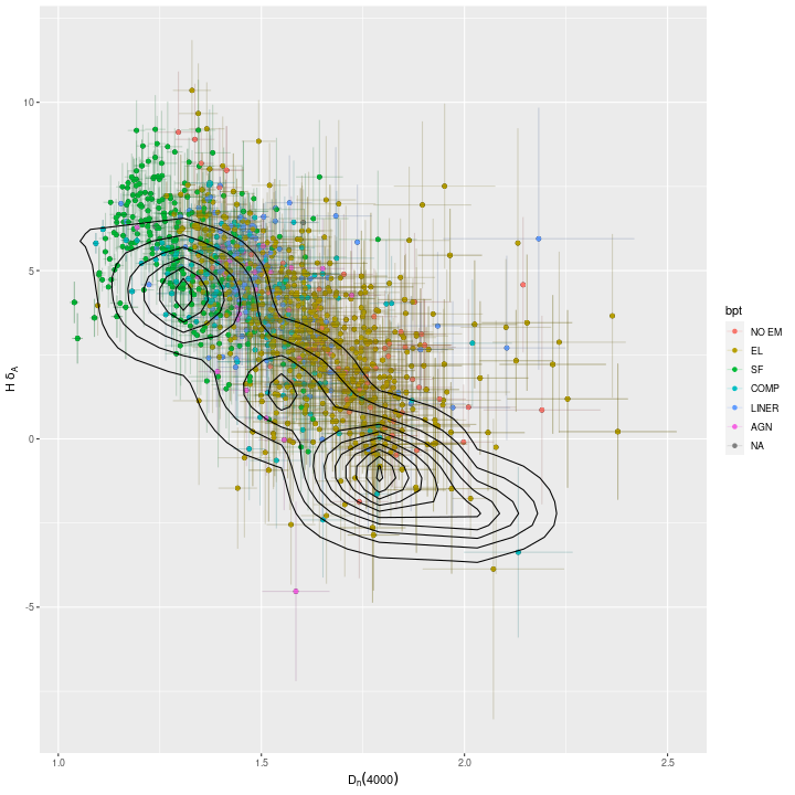
First, here is a popular absorption line diagnostic, the Lick HδA – Dn(4000 Å) plane. Points are colored by BPT diagnostic determined from the [N II]/Hα and [O III]/Hβ ratios by the usual criteria. The contours are from measurements of a large sample of SDSS galaxies by the MPA-JHU pipeline, which was run on spectra through DR8.
Lick HδA versus 4000Å break strength – MaNGA post starburst sample. Contour lines are for a large SDSS sample with measurements from the MPA-JHU pipeline.
It seems odd that the bulk of the measurements in this sample are displaced from the bulk of the SDSS sample. I wouldn’t completely rule out errors in my measurements but I tested mine against the MPA-JHU measurements a long time ago, and this particular part of the code is unchanged for some time. Anyway, we see a large range of values of these diagnostics, but with relatively few in the passively evolving region at lower right and many in the “green valley.” Almost 1/3 have strong Balmer absorption with HδA > 5Å EW. Many of these also have star forming BPT diagnostics, so it’s not clear that these regions are post starbursts.
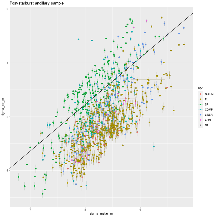
Next, here are (100 Myr averaged) star formation rates plotted against stellar mass density, again color coded by BPT diagnostic. The straight line is my calibration of the center of the “star forming main sequence” from some time ago.
Modeled SFR density vs. stellar mass density – MaNGA post starburst sample.
Evidently there are many regions — mostly with star forming emission line ratios — lying near the star forming main sequence, and also a large number in the green valley. Most of those have weak emission lines, AGN, or LINER-like ratios.
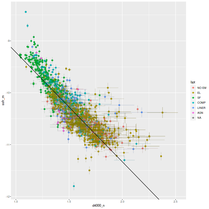
Finally, here is a plot of model specific star formation rate against Dn(4000Å). As I’ve written before a number of authors have noted the relation between the 4000Å break strength and stellar age or specific star formation rate and several have used it as a (usually secondary) star formation rate indicator. The straight line is my estimate of the mean relation for spiral galaxies, originally given in this post.
Model specific star formation rate versus 4000Å break strength – MaNGA post starburst sample.
Evidently by these diagnostics this sample has properties that at least overlap with a random selection of normal galaxies. The only thing notably missing are “red and dead” ETGs. However there are good reasons to think that starbursts – and therefore post starbursts – are generally localized regions within galaxies. We need to look at the spatially resolved properties — specifically star formation histories — to see how many genuine post starburst galaxies are in the sample.
I’m going to end for now with one of the more interesting examples in this sample. The western member of this interacting pair has a remarkably bright and white nucleus, which in SDSS imaging indicates a fairly young stellar population.
SDSS J095343.89-000524.7 MaNGA plateifu 10843-9101 (mangaid 1-897)
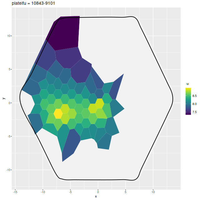
I slightly altered my usual workflow for this and a few other data sets in this sample. Usually I try to use all spectra and bin to a minimum target SNR (usually 5) for all bins, but since this IFU had a large fraction of blank sky I set the SNR threshold for accepting a bin lower than I otherwise would and left the lowest SNR spectra out of the analysis. Below is a map of the modeled stellar mass density showing the coverage of the analyzed area.
MaNGA plateifu 10843-9101 (mangaid 1-897). Model stellar mass density; analysis coverage
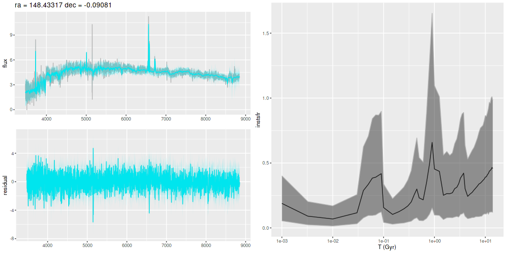
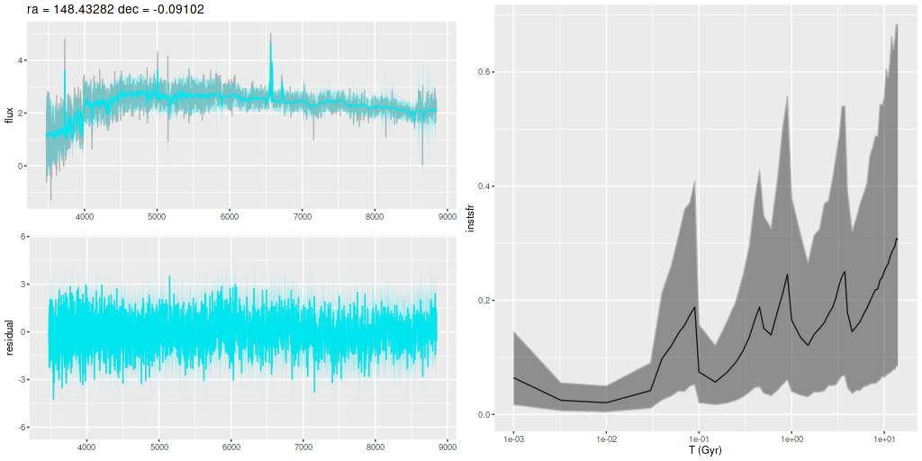
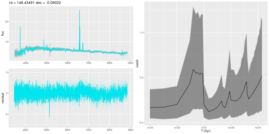
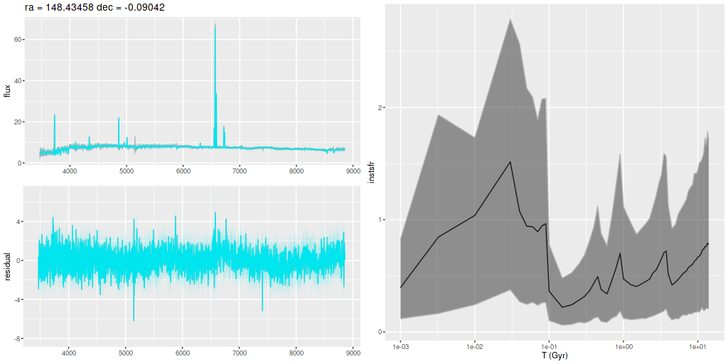
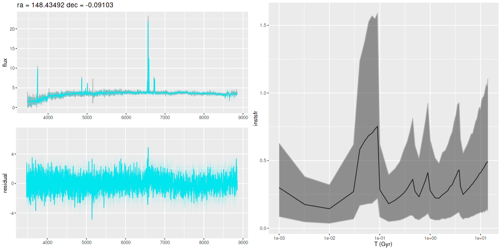
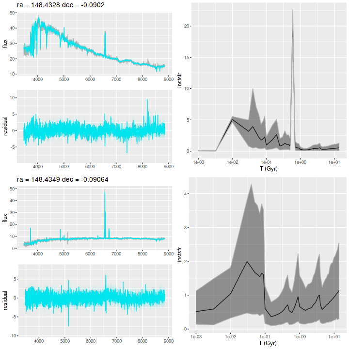
And for now I’ll just show the spectra of the two nuclear regions with posterior predictive fits of the SFH models, along with model star formation histories. The western nucleus has a remarkable K+A like spectrum but with fairly strong emission from a possible AGN. The model star formation history is one of the most unusual I’ve seen. Whether it’s an accurate record of events is of course uncertain.
MaNGA plateifu 10843-9101 (mangaid 1-897). Nuclear spectra with posterior predictive fits and model star formation histories.
I’m going to continue this topic in additional post(s), and perhaps look for a larger sample. A recent paper by Cheng et al. (2024) found nearly 500 galaxies with post starburst properties in MaNGA, but there seems to be no catalog. I’m not sure their selection criteria are easily reproduced.
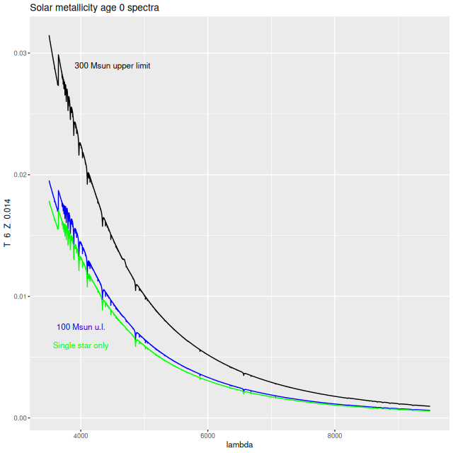
Three posts ago I did a brief comparison of my usual EMILES based models with the most recent version of Stanway and Eldridge’s BPASS models, which are the first purely theoretical model spectra that seem possibly suitable for full spectrum fitting. I mentioned then that I used a set of models with an age zero upper mass limit of 300 M☉, while most model libraries adopt an upper mass limit of 100 M☉. As is customary in this industry their website contains a number of additional model libraries, including with upper stellar mass limits of 100 M☉ and some with single star evolution only. These alternate sets of models have the same structure as the baseline models, so I just used the same scripts to create R readable data sets with the same ages and subset of metallicities..
Not surprisingly the 1 Myr models with 300 M☉ upper limit are considerably more luminous than either the binary or single star models with 100 M☉ limits, but the latter are still somewhat more luminous than my standard library at the same age. Stars >100 M☉ evolve very rapidly and the difference in model spectra disappears by log(T) = 6.6 (4 Myr).
BPASS solar metallicity age 0 model spectra
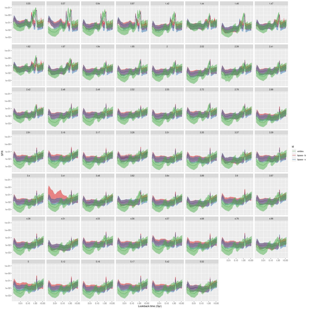
To test the differences in model star formation histories I just ran one set of models on the post-starburst galaxy WISEA J080218.38+323207.8 (MaNGA plateifu 10220-3704, mangaid 1-201936). And here’s the comparison:
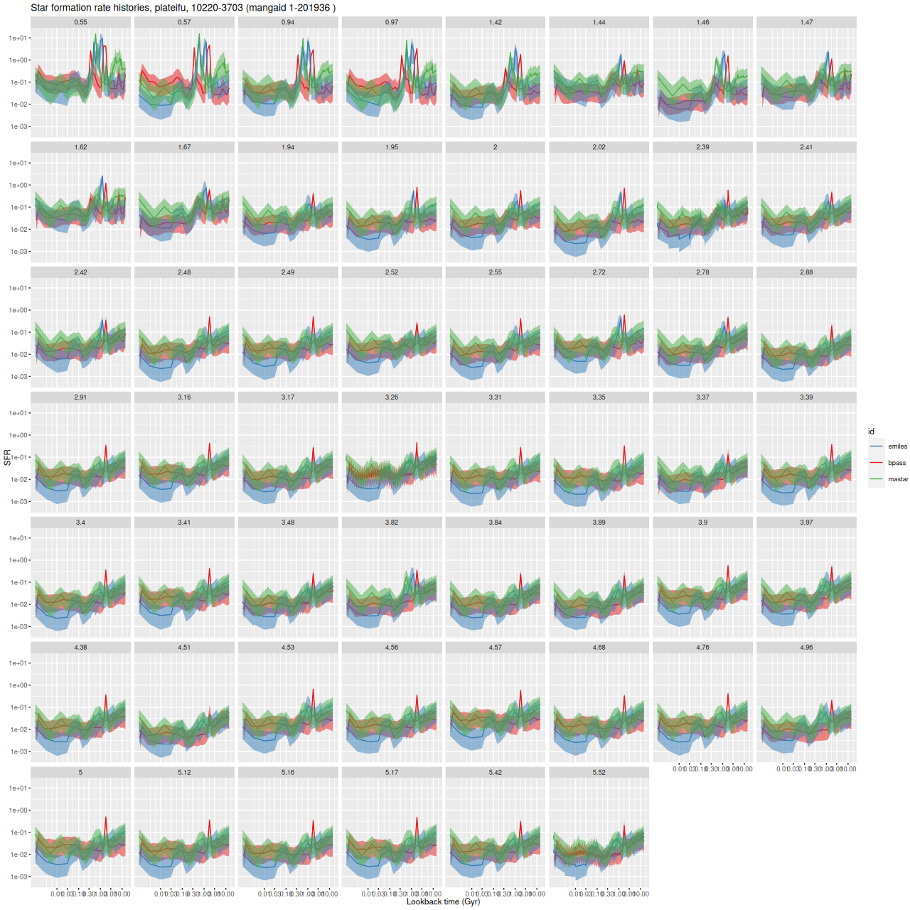
Model star formation histories for 3 SSP model libraries. MaNGA plateifu 10220-3703 (mangaid 1-201936)
The basic result is there’s no real difference either with the 300 M☉ upper limit models or between the binary and single star evolution models1note that one spectrum in the fifth row above has a rather different model SFH for the binary library. This turned out to be from a convergence failure of the sampler in one chain. Again there’s a sharp downturn in star formation rate at the youngest ages and again there’s that peculiar spike at 1.6 Gyr in all model runs. That feature has serious consequences for the interpretation of the model star formation histories in these post-starburst galaxies. In this case the EMILES based models indicate a strongly centrally concentrated burst that began ~1 Gyr ago and lasted several hundred Myr in the center, while fading away to no significant enhancement outside a few kpc from the center. The BPASS models on the other hand have two distinct bursts near the center that straddle those of EMILES, with a significant amount of mass in a short burst throughout the galaxy. While not necessarily implausible the persistence of the 1.6Gyr spike (and as noted before not just in this galaxy) makes me suspect an artifact of some sort.
As a little bit of an aside this galaxy has one published estimate of a detailed star formation history by French et al. (2018) based on GALEX and SDSS photometry and SDSS spectra (not MaNGA). Their best fit model has two bursts at ~500 Myr and 1.5 Gyr with a total mass contribution of ~20 – 65%. Since the SDSS spectra were 3″ diameter this would be for the central region only. This at least broadly agrees with either the EMILES or BPASS based models. I have roughly 75% of the mass in the burst (EMILES) in the central fiber with somewhat more in the BPASS models, but that drops rapidly.
Well, the quest for an updated SSP library continues. Unfortunately the two likely sources of MaStar based models have yet to publish updates. I’m still considering doing my own. Unfortunately I’m not aware of any open (or for that matter closed) source software for generating SSP model spectra. This seems to be something of a dark art.
After my not so insightful realization recounted last time that my attempt to modify the prior on star formation histories wasn’t actually doing anything I thought a little further about how to specify one. Gaussians are always popular choices for priors, so why not give them a try? For a first cut I added the following lines to the “transformed data” section of the Stan model:
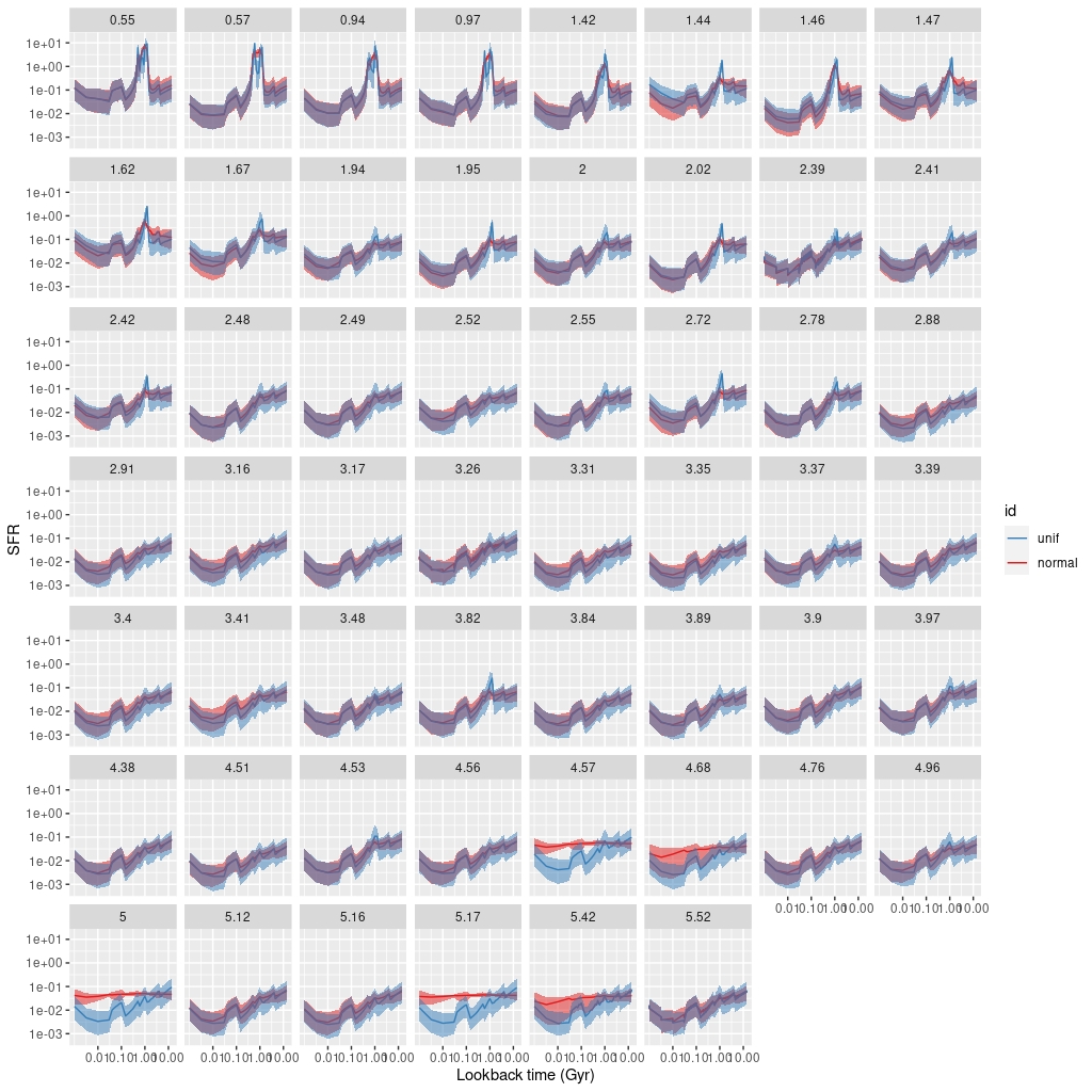
Even though the prior allows values of the stellar contributions that are infeasible given the simplex declaration this causes no technical problems: the models sample without complaint and parameters satisfy all constraints. Execution times are comparable to the original model formulation and convergence diagnostics are OK. But, the model runs had some unexpected features. I did a set of model runs for a single MaNGA galaxy from the post-starburst ancillary sample — mangaid 1-201936 (plateifu 10220-3703). Model star formation histories compared to the original model are shown below for the 58 binned spectra:
MaNGA plateifu 10220-3703 (mangaid 1-201936). Model star formation histories with two different SFH priors.
What’s striking here is that several of the spectra in the low S/N outskirts of the galaxy have nearly constant star formation rates with very little sample variation. In other words the models are basically returning the priors. The cause of this behavior isn’t quite clear. Relatively low signal to noise seems to be necessary, but not sufficient since similarly noisy spectra have essentially the same SFH’s as the original model formulation. It also isn’t due to convergence failure because much longer runs with more adaptation iterations show the same behavior. It is possible perhaps that the posteriors are significantly multimodal and Stan is preferentially falling into one of them. Notable also is that the fits to the data measured by log-likelihood are virtually identical even for the runs with the anomalous SFH’s. At the very least this tells us that uncertainties in quantities derived from the models are considerably larger than within model run variations — of course I have always believed this and said so a number of times.
After trying several variations on this theme that either had none at all or undesirable effects on sampling, and after some additional consideration I think that, given the model parametrization, the uniform on the simplex prior for stellar contributions is actually the one I want. That leaves the question of what, if anything, to do about the abrupt jumps in model star formation rates.
One possibility is simply to redefine the endpoints of the age bins to be, say, halfway between nominal SSP ages instead of at the model ages as is my current practice. In the case of the EMILES library this would mean for example that the 3.75, 4, 4.5 Gyr bins would have widths of 0.25, 0.375, 0.5 Gyr instead of the present 0.25, 0.25, 0.5. This involves no change to the actual model runs at all, so most quantities derived from the models are unchanged.
Another solution is to adopt a library with a more uniform age progression. One with approximately equal increments in log age seems preferred. As yet there have been no published updates to the MaStar based SSP libraries mentioned last time, so I’m waiting for them, while still considering generating my own.
I’m going to briefly return to BPASS based models. After that I’m not sure.
One thing I’ve wondered about for a while is the extent that priors on SSP model contributions affect modeled star formation histories. Previous experience suggests not much at all unless the prior is highly constraining. To be a little more specific in my current workflow I normalize the SSP model spectra to have average flux values of 1 in (approximately) the V band, and also adjust the galaxy fluxes in the same way. In the Stan model the stellar contribution parameters are declared as a simplex, that is a vector with non-zero elements summing to 1. That makes the parameter values the fractional contributions to the (unreddened) galaxy flux at V. My current working code doesn’t provide an explicit prior for the stellar parameters, but they have an implicit proper prior of a uniform distribution on the appropriate dimensional simplex. More technically the prior is a Dirichlet distribution with all concentration parameters equal to 1. Note the marginal distributions aren’t uniform, but they are all the same. One implication of that is that a typical draw from the prior1Stan doesn’t sample from the prior even for initialization, but of course the prior influences the posterior through Bayes’ rule. will have jumps in the star formation rate at exactly the times where the width of the age bins jump, a problem that I’ve noted several times before.
A possible solution to this problem is simply to alter the prior to encourage smoothly varying star formation rate rather than smoothly varying light contributions. It turns out I’ve been feeding my Stan code the data I need to do that: the initial mass in a given model SSP is inversely proportional to the normalization factor applied to the spectrum, and the star formation rate is just the mass divided by the time interval assigned to the SSP. Both of those quantities are passed as data to the Stan model even though they weren’t used in any way previously. I added just 3 lines to the code to change the prior on the stellar contributions. In the “transfored data” section
If I did this right the prior is completely agnostic to any star formation history, whereas the previous implicit prior was completely agnostic to any run of light contributions.
The modified code compiled without complaint and there’s no discernible difference in either execution time or convergence diagnostics.
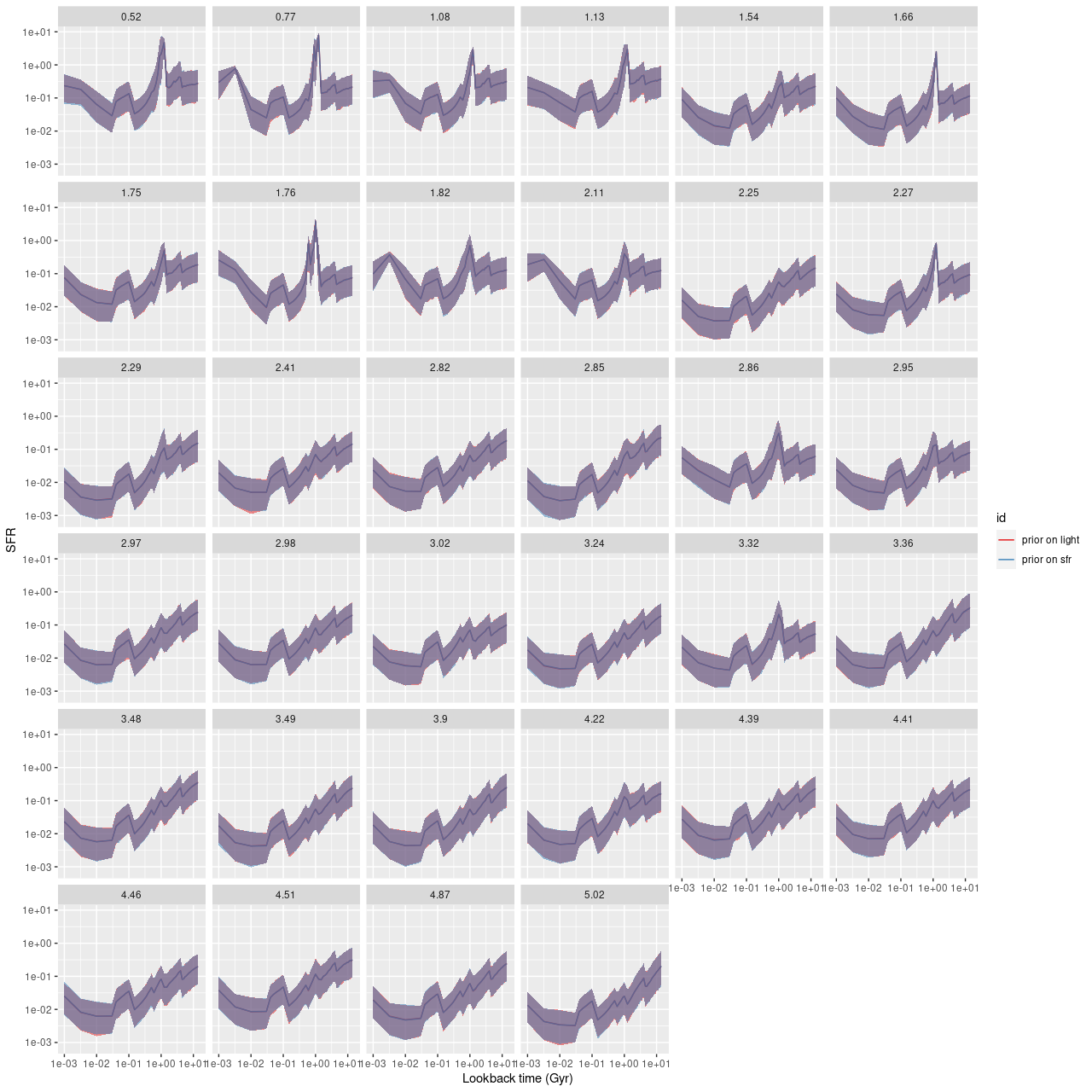
I’ve only run this on one set of galaxy data, from MaNGA plateifu 8565-3703 (mangaid 1-92735). This is one of Schawinski’s “blue early type galaxies,” chosen mostly because the data were binned to just 34 spectra so a complete set of model runs only took a few hours. And, as seen below the other things that don’t change are the modeled star formation histories.
Plateifu 8565-3703 (mangaid 1-92735). Star formation history models with two distinct priors on stellar contributions.
I need to do some more validation exercises, but it appears my long ago conclusion that the choice of prior on the star formation history has little effect was correct. The data dominates the model outcome through the likelihood.
Update
Since I hit publish a few days ago I realized two things. First, the weights I applied to the stellar contributions to “encourage” a smoothly varying star formation rate were inverted. What I should have used was:
The second thing I realized is this makes no difference at all given the form of the prior. The transformation simply maps a point on the simplex to another point on the simplex that has exactly the same probability density since by construction the prior is uniform on the simplex.
So, it should have been expected, and it’s a good thing that it in fact happened that the model runs produced the same results. What happens if I use the following prior, with the weights supplying the parameters for the Dirichlet?
target += dirichlet_lupdf(b_st_s | norm_sfr);
This failed to sample almost always. I’m not entirely sure why, but I suspect this turns a problem with relatively simple geometry at least with regards to the prior to one with a complex and troublesome geometry.
This little experiment actually told me nothing about the effect of priors on model star formation histories. Two of the priors are actually the same, and the third fails for reasons that aren’t completely clear. I may experiment with different forms of prior. I’m still, of course, looking for a new SSP model library.
For a few years now I’ve been using a library of SSP1Simple Stellar Population model spectra based on the EMILES models of Vazdekis et al. supplemented with some young stellar populations taken from the “HR-pypopstar” models described in Irigoyen et al. (2021) and retrieved from fractal-es.com/PopStar. As I’ve mentioned several times there are a few issues with the models. First, the abrupt changes in time intervals of the BaSTI isochrone based models produce sharp jumps in model star formation rate estimates at several lookback times. This is because my star formation history models “want” to produce smoothly varying contribution estimates, which lead to abrupt jumps in rates when the time interval decreases.
Another possible issue is there are multiple sources of data used for the SSP model spectra. Besides the pypostar models for young populations the older population spectra use MILES stellar spectra for wavelengths up to 7410Å, with spectra from another source grafted on for longer wavelengths within the relevant range for SDSS. This wavelength happens to fall on a wide absorption feature (I believe mostly due to TiO) that’s prominent in older populations, and this region is often fit rather poorly by the models. Although there are other possible reasons for this I’ve long suspected that it might be due to different flux calibrations of the two data sources. Ideally I’d like to have single, homogeneous data source covering the full wavelength range of SDSS spectra.
That ideal data source may exist in the SDSS MaStar stellar spectrum library, which is a large collection of stellar spectra observed as part of the MaNGA project. Since the observations used the same BOSS spectroscopes they have the same wavelength coverage, spectral resolution, and flux calibration as the MaNGA galaxy spectra. So far I’ve found 2 MaStar based SSP model libraries. First is one described originally in Maraston et al. (2020) with data available at https://www.icg.port.ac.uk/mastar/. This was based on the preliminary (DR15) data release and has a minimum age of 300Myr, which is unsuitable for my purposes. An updated version with sufficiently young models is described in Nanni et al. (2022, 2023, 2024). That version has not yet been published as of the date of this post.
A more immediately usable set of models were described in Sanchez et al. (2022) and retrieved from http://ifs.astroscu.unam.mx/pyPipe3D/templates/. These are based on the 2019 update of the venerable Bruzual and Charlot (2003; BC03) models, with MaStar spectra substituting for MILES+IndoUS in the relevant wavelength range. The spectra were taken from the initial (DR15) data release and an update is promised to be forthcoming.
The linked directory contains a large number of FITS files containing subsets of the full data set(s) — both the CB19 and MaStar based models are included. Since I wanted to select my own subset I downloaded the presumed full data sets in files named “MaStar_CB19.all_1_5.fits.gz” and “MaStar_CB19.all_1_5.fits.gz.” These contain model spectra and some other data for 210 irregularly spaced ages (not 220 as stated in the paper) and 16 metallicities. Very young ages are over-represented — there are 23 under 1 Myr and another 55 between 1 and 10 Myr. Beyond 3 Gyr the interval between models is fixed at 0.25 Gyr. For a preliminary evaluation I chose 47 ages from 1 Myr to 14 Gyr and 5 metallicities ranging from somewhat subsolar (Z = 0.004) to the highest available (Z = 0.06). I used the model spectra as given with wavelengths from 3625-9998.5Å at 1.5Å spacing. I built libraries for both the CB19 and MaStar based spectra, but will only discuss the latter for now.
I also decided to reevaluate the most recent release of the “BPASS” evolution models of Stanway and Eldridge (2018) with data retrieved from links at https://bpass.auckland.ac.nz/9.html. These are purely theoretical models including predictions for spectra, and are unique in attempting to account for binary star evolution. I had looked at a much earlier version and decided that the model continua were much too blue to be useful for full spectrum fitting. This appears to be no longer much of an issue.
Again, there are a large number of files in the data directory with different choices of IMF and upper mass limits. For a first look I chose the file bpass_v2.2.1_imf135_300.tar.gz, which corresponds to a Kroupa IMF with upper mass limit of 300 M☉2which may have been a mistake since the upper mass limit in all the other libraries I’ve tried is 100M☉. Models are available for 11 metallicities, and again I chose 5 with values ranging from Z=0.004 to Z=0.04 (the highest available). The available ages are in equal logarithmic intervals from 106 all the way up to 1011 years with a spacing of 0.1 dex. I just chose all available ages for log(T) = 6 to 10.1, for a total of 42. According to the documentation ages are meant to represent the middle of each time interval. So far I’ve adopted the convention that ages represent the beginning of each time interval of width equal to the time to the next younger age, so for consistency I add 0.05 dex to each model age. I extracted the model spectra in the wavelength range 3500-9499Å, which are tabulated at 1Å intervals.
For a preliminary evaluation I calculated models for just two MaNGA galaxies. Plateifu 10220-3703 (mangaid 1-201936; NED name WISEA J080218.38+323207.8) is a post-starburst taken from the compilation of Melnick and dePropris — one of 8 in the final MaNGA release. The other is a late type spiral, plateifu 11018-12704 (mangaid 1-233951; UGC 8162). This was a more or less random choice drawn from a sample that was intended to be a high purity selection of MaNGA face on spirals based on Galaxy Zoo classifications and NSA axis ratios. These two span the range of galaxy types that I’m likely to want to examine in the near future.
2MASX J08021836+3232078 – MaNGA plateifu 10220-3703 (mangaid 1-201936)UGC 8162 – MaNGA plateifu 11018-12704 (mangaid 1-233951)
I’m just going to look at a few results of model runs. Execution times, convergence diagnostics, and fits to the data as measured by summed log-likelihoods were all similar so there’s no strong reason to favor one library based on those criteria.
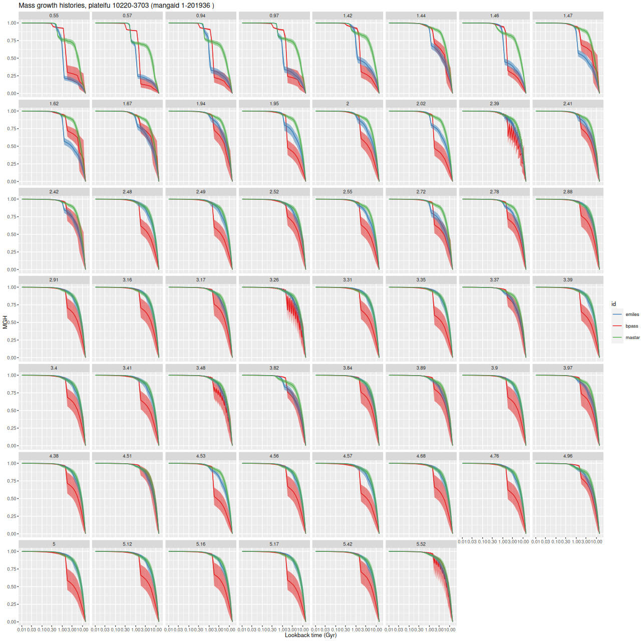
Turning first to the post-starburst galaxy 2MASX J08021836+3232078, here are model star formation rate histories for all binned spectra and all three tested SSP libraries. The ribbons denoting the marginal 95% credible intervals of SFR mostly overlap3note these are log-log plots that span 4 orders of magnitude in star formation rate, which is encouraging, but the model mass growth histories are rather different as seen below4as something of an aside several panels show a strange zigzag pattern. This is a rendering issue with the graphics software rather than a sampling problem. Note in particular that the mass growth histories by construction are monotonic.
Comparison of model star formation rate histories from 3 different SSP model libraries – all binned spectra, MaNGA plateifu 10220-3703.Comparison of model mass growth histories from 3 different SSP model libraries – all binned spectra, MaNGA plateifu 10220-3703.
Both the EMILES and BPASS models have a strong, centrally concentrated quenched starburst with two peaks, but with slightly different timing. The MaStar based models on the other hand show a long period of quiet evolution with a later and weaker starburst in the central region. A very peculiar feature of the BPASS models is a spike in SFR in almost every model run at logT = 9.2 (1.6 Gyr). A little more on this below.
There are some fairly large differences in summary quantities I track. The average stellar mass density is 0.14 ± 0.05 dex larger in the MaStar based models than EMILES, while it’s 0.12 ± 0.05 dex smaller in the BPASS models. The (100 Myr average) star formation rate density is 0.3 ± 0.1 dex larger in the MaStar models and 0.09 ± 0.16 dex larger in the BPASS models. The BPASS models have greater optical depths of dust attenuation (by 0.14 on average) and redder attenuation curves (<δ> ≈ 0.5). This may indicate that the BPASS spectra still have bluer continua than EMILES.
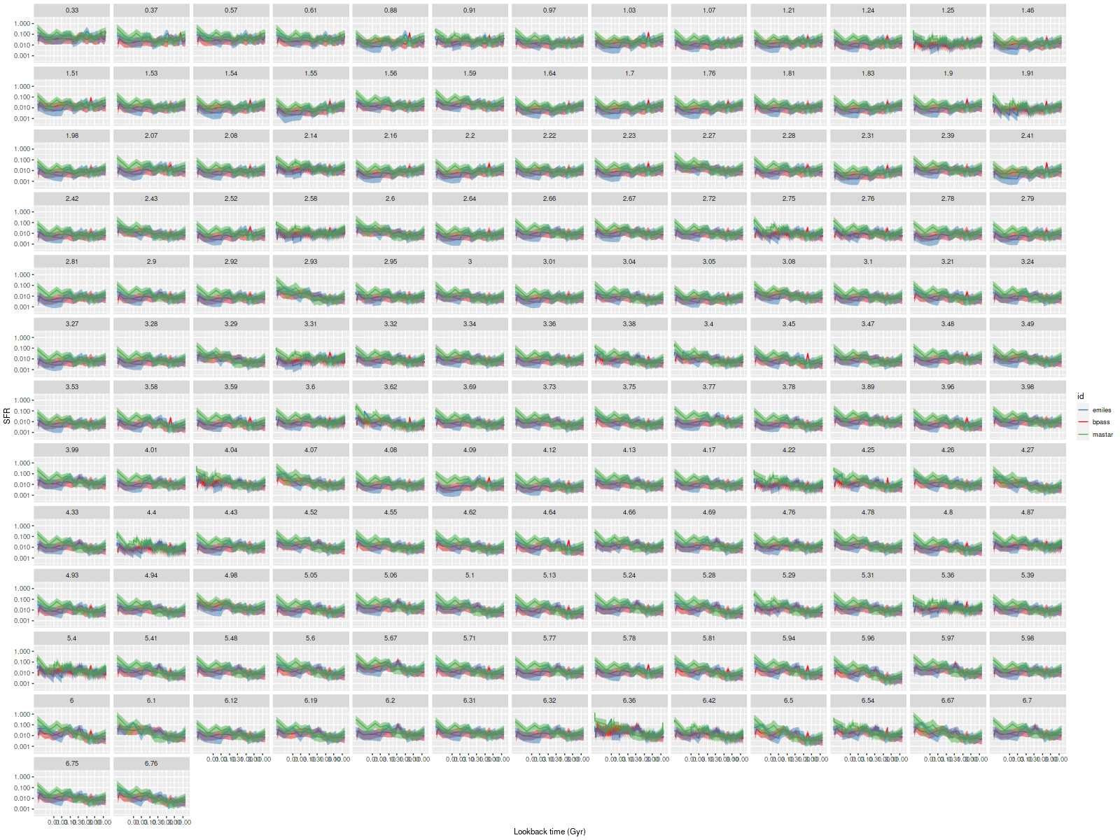
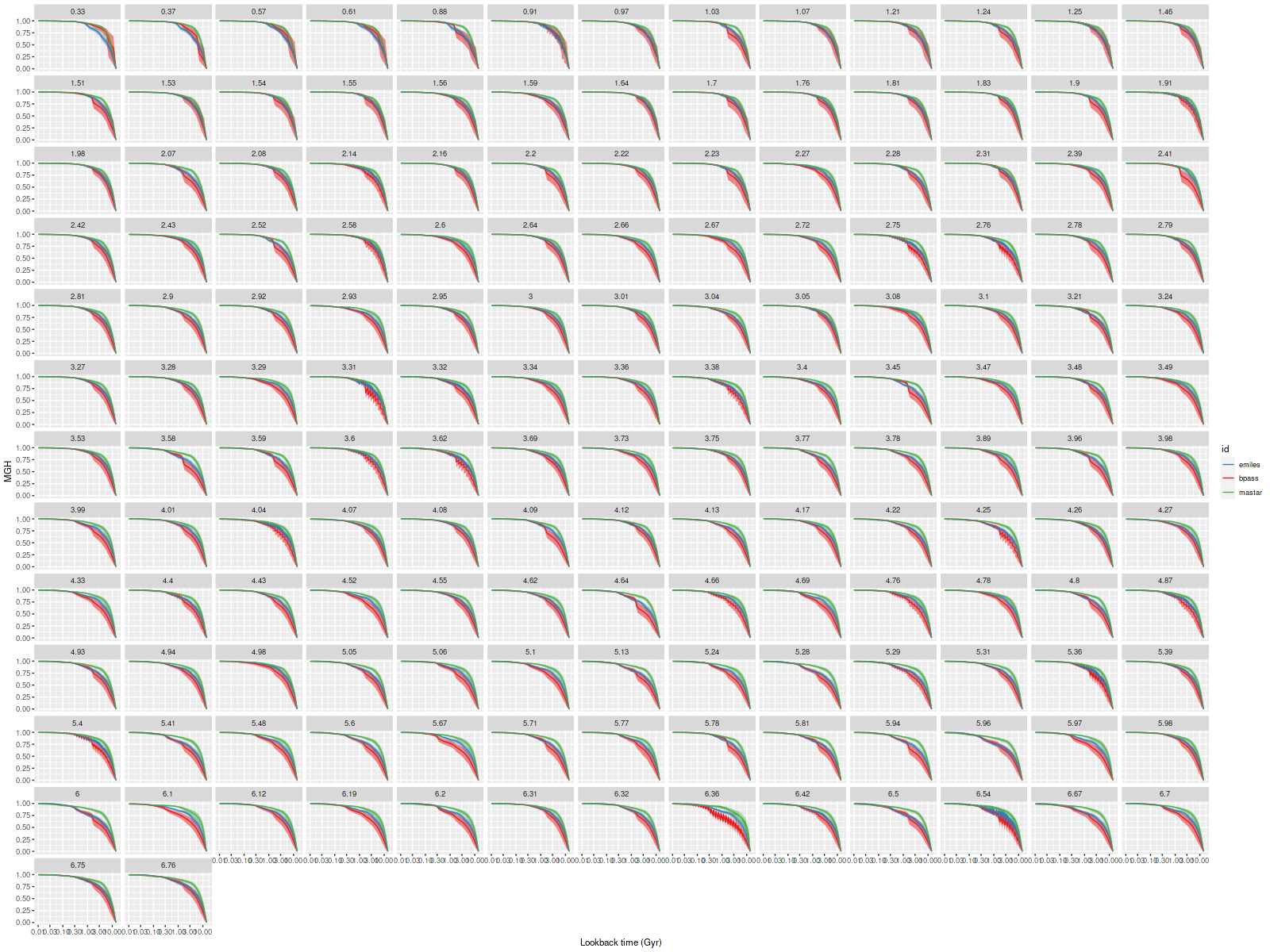
Turning to the spiral, here are the same two sets of plots for UGC 8162. Again the model SFR histories overlap and all three indicate roughly constant star formation over cosmic history with perhaps even slightly increasing in the outskirts. Close examination of the mass growth histories show the MaStar based models favor slightly faster early time growth than the other two.
Comparison of model star formation rate histories from 3 different SSP model libraries – all binned spectra, MaNGA plateifu 11018-12704.Comparison of model mass growth histories from 3 different SSP model libraries – all binned spectra, MaNGA plateifu 11018-12704.
Although less obvious many of the BPASS model runs have a distinct spike in SFR at the same 1.6 Gyr as in the post-starburst models. In some of the spectra it’s strong enough to contribute significantly to the present day stellar mass. A few other peculiarities are harder to see. The MaStar models invariably have an upturn in SFR at the youngest age (1 Myr), while the BPASS models invariably have a sharp downturn at the youngest age.
There are similar offsets in stellar mass densities to the post-starburst, by 0.12 and -0.14 ± 0.03 in MaStar and BPASS respectively. The mean star formation rate densities are 0.25 ± 0.05 larger in MaSTar but 0.18 ± 0.07 dex lower in BPASS models.
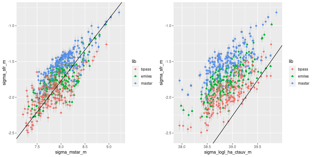
For a quick look at how these model differences affect some key relationships, below are plots of the mean (and standard deviations) of SFR density against stellar mass density (L) and SFR density vs. Hα luminosity density (corrected for estimated stellar attenuation only) (R) for UGC 8162. The straight lines are my estimate of the “star forming main sequence”, and on the right the Calzetti calibration. As expected the models straddle the “spatially resolved star forming main sequence” that I estimated previously5data for this galaxy was recently downloaded and the model results did not contribute to my estimate.. Note that since the BPASS model estimates of both SFR and stellar mass are offset by similar amounts from the EMILES based models the points are just shifted downward along essentially the same relationship. The MaStar based models appear slightly offset to higher SFR values at a given stellar mass density. On the right, there’s a fairly clear stratification. The Hα luminosity estimates are nearly identical for all 3 sets of model runs, so we see the differences in SFR density estimates.
MaNGA plateifu 11018-12740
Model results from 3 SSP libraries
(L) SFR density vs. stellar mass density
(R) SFR density vs. Hα luminosity density corrected for stellar attenuation
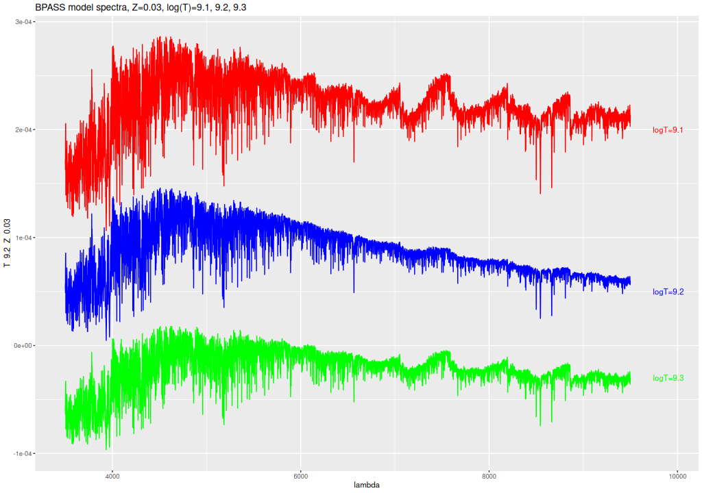
I don’t really have an explanation for the 1.6 Gyr spike in the BPASS models. It’s happening in the two super-solar metallicity bins, which track with the others for both younger and older ages. One possible clue is in their spectra. The broad absorption features in the red are considerably deeper at both younger and older ages6spectra are offset vertically for clarity.. Whether there’s a physical reason for this and why it would affect the models as seen is unknown to me.
BPASS SSP model spectra for Z=0.03, T=1.25, 1.6, and 2 Gyr
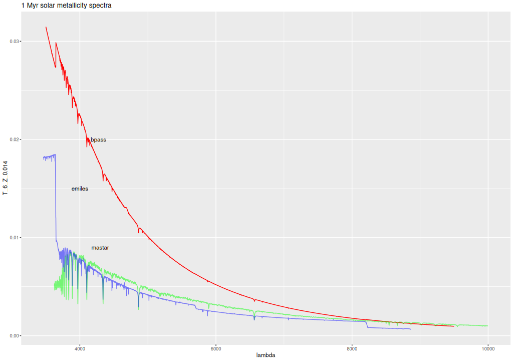
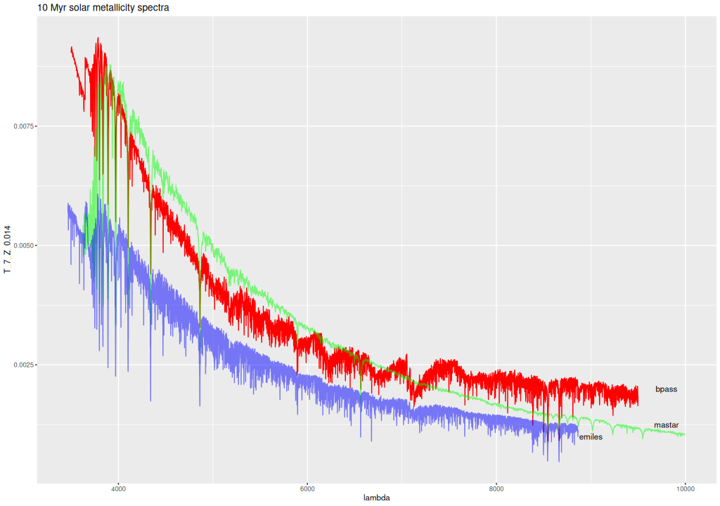
There are some notable differences among the libraries at young ages at well. Below are plotted the 1 and 10 Myr spectra at solar metallicity for the 3 libraries. The “EMILES” spectra recall are from the theoretical PyPopstar models with continuum emission included. The BPASS model is considerably more luminous and bluer at 1Myr than the other two and evolves more rapidly at young ages. Is this because I chose the models with 300 M☉ upper mass limit? I should find out.
BPASS, EMILES, and MaStar solar metallicity model spectra at 1MyrBPASS, EMILES, and MaStar solar metallicity model spectra at 10 Myr
To conclude for now I haven’t quite decided what to replace my existing EMILES models with, if anything. I’m still optimistic that an MaStar based library is the way to go, but the version published by Sanchez et al. isn’t quite ready for production use. I may consider developing my own library although it’s outside the scope of my interests.
When I was doing my initial fits to the M31 MaNGA spectra I noted two that I initially thought were contaminated by foreground stars, and therefore I masked them to prevent further analysis. One of the two, in MaNGA plateifu 9677-12701 (mangaid 52-8) is a certain foreground star and won’t be discussed further. The other, in plateifu 9678-12703 (mangaid 52-23), turns out to be a luminous red supergiant that’s a genuine resident of M31. This is confirmed by two nearly contemporaneous catalogs of M31 red supergiants: the one by Ren et al. (2021) that I noted previously and Massey et al. (2021), which I stumbled upon more recently.
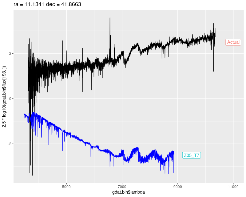
In fact there are two comparably bright red supergiants in this IFU. One that’s about 9″ north of the masked one probably should have been masked by whatever criteria I used, but it’s likely I failed to notice the fit to the data since I don’t have the patience to look at every spectrum and data fit that pops up. So, here is the spectrum, displayed in (negative) magnitudes with arbitrary zero point. The blue spectrum is the closest match in my SSP library, a 10 Myr old population with the highest metallicity I used (2.5 Z☉. This is one of the theoretical spectra from PyPopstar). This sorta looks right except it’s much too blue. The solution to that is, of course, to add some reddening through dust attenuation.
plateifu 9678-12703 (M31 10 kpc ring)
Spectrum contaminated with red supergiant and closest match SSP model spectrum
The maximum likelihood (non-negative weighted least squares) fit did just that, with only a single stellar contributor and a very high dust attenuation of τV = 3.0. This still doesn’t quite work: the residuals are rather strongly sloped in the blue and the details of the absorption features in the red aren’t quite right.
plateifu 9678-12703 – NNLS fit to spectrum contaminated with red supergiant
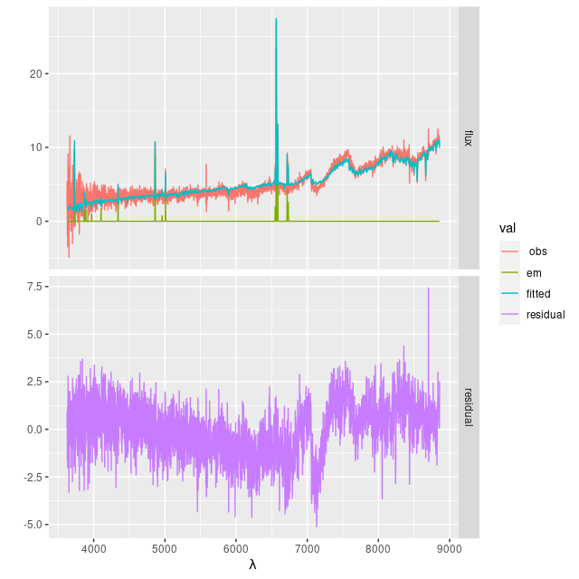
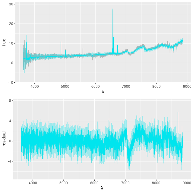
I still use a Calzetti attenuation relation in my NNLS fits. The Bayesian fits using Stan have the more flexible attenuation prescription that I described back in this post, and that helped considerably with the continuum as seen in the plot below. The absorption features in the red still aren’t fit well. The model has an even more extreme attenuation estimate with a much “grayer” than Calzetti slope, with τV = 4.38 ± 0.05 and δ = -0.33 ± 0.011see the link above for the meaning of these parameters.
9678-12703 – posterior predictive fit to spectrum
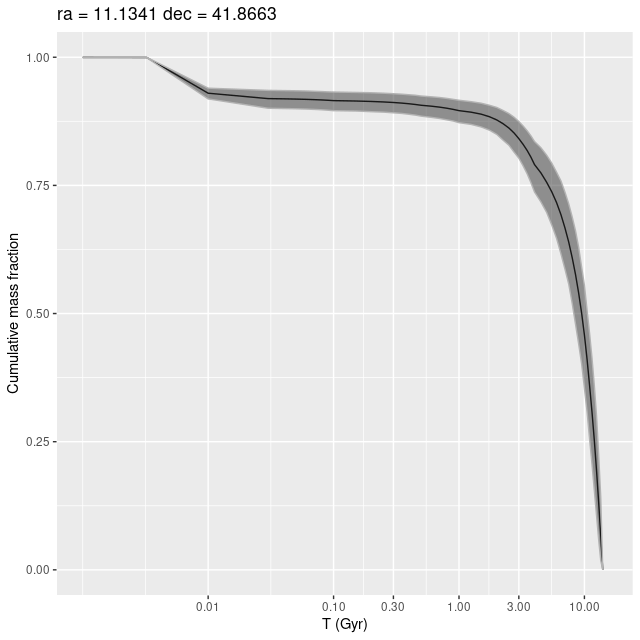
The model star formation history (displayed as a mass growth history below) isn’t completely implausible. The presence of a very luminous evolved star indicates the region is at least some Myr old, and a rapid onset and decline of star formation is typical for star forming regions in mature spirals. The recent episode of star formation added about 7% to the present day stellar mass, while at least 60% was in place by 8 Gyr ago (per the model).
plateifu 9678-12703 (M31 10 kpc ring)
Model mass growth history for a region containing a bright red supergiant
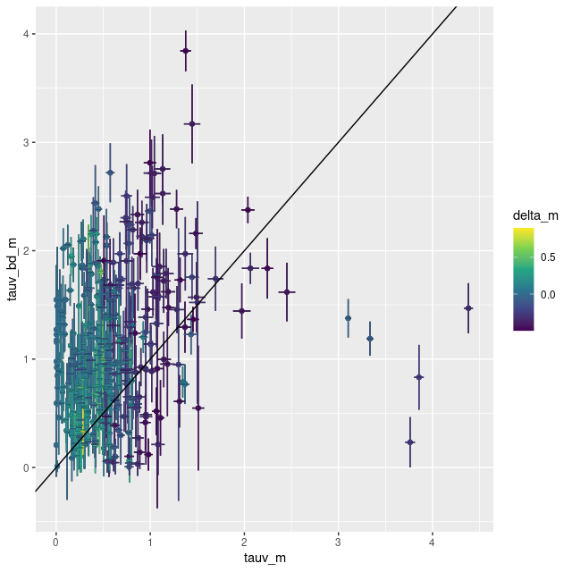
Nevertheless I consider the model results to be highly suspect, mainly based on the very large optical depth. Massey estimates the attenuation for the red supergiant to be AV ≈ 1.18, although this is apparently based on a formula rather than a direct empirical estimate. But another piece of evidence that’s close to a smoking gun is an estimate based on the Balmer decrement of emission. Despite the lack of apparent ionizing sources outside the bright H II regions in the west there is widespread diffuse emission in this region with star-forming like line ratios. The estimated optical depth derived from the Balmer decrement for this region is τV, bd = 1.47 ± 0.23 (1σ), reasonably consistent with the Massey estimate and with the values derived for the rest of the IFU.
How widespread a problem is this? Below I plot the Balmer decrement derived optical depths against the stellar based estimates for all spectra in M31 MaNGA with star forming emission line ratios, about 11% of the entire sample. The 5 most extreme outliers are in this IFU in the regions surrounding the two bright red supergiants (the masked spectrum would also be in this region of the plot). The same 5 regions are also extreme outliers in the SFR vs. stellar mass and SFR vs. Hα plots that I showed early on. So, even though there are many cataloged supergiants in the study region these two appear to be uniquely bright and to have had the largest impact on model results.
M31 MaNGA – Optical depth off attenuation estimated from Balmer decrement vs. model values of τV
Of course there are hotter bright stars in the study area and these could affect results in different and possibly unexpected ways. For example the outermost IFU contains one bright star that GAIA estimates has a surface temperature of 5500 C, which would make it a G supergiant if it’s in M31. I noted in the last post that the model star formation history for that region looks like a post starburst with an age around 800 Myr. This is, I think, several galactic rotation periods, and stars born that long ago should have dispersed by now unless they’re gravitationally bound. There’s no sign of a star cluster there nor is there a cataloged one nearby, so it seems likely to me that the “starburst” is an artifact. As I noted in the last post though the fit to the data is quite good.
These examples illustrate an issue that’s fairly well known, which is that using simple stellar populations as building blocks of low mass stellar systems are potentially affected by so-called “stochastic” effects, which simply means that the distribution of stellar masses can vary randomly from what’s assumed in the SSP models. Specifically, in M31 there are individual stars luminous enough to affect spectra. One possible solution might be to add some stellar spectra to the library. I might give that a try some day.
I’m going away and won’t be writing for a while. I’m hoping to acquire or build a SSP model library based on SDSS MaStar spectra yet this year. This is a much larger collection of stellar spectra than has been previously available and it has the advantage of having the same flux calibration and (approximately) spectral resolution as the SDSS galaxy spectra. I also plan to return to my study of post-starburst galaxies.
On to the final batch, which I don’t think is going to be very interesting.
plateifu 9678-12704 (mangaid 52-22)
If my calculations reported in the last post are correct this is well in the outer disk at a distance of about 15.4 kpc from the nucleus. Other than that there’s nothing much to say about it. There are no cataloged objects of interest in the IFU footprint. There is diffuse emission with a fairly strong gradient decreasing from northwest to southeast, which is basically moving outward in the disk. There may be low level ongoing star formation.
plateifu 9678-12704 (M31 outer)
(L) Hα luminosity density (uncorrected)
(R) SFH summed over IFU footprint
plateifus 9678-6103 and 9678-12702 (mangaid 52-19 and 52-24)
These are both in interarm regions with absolutely no cataloged objects of interest and complete blanks in the Galex false color image. Even diffuse emission is too weak to detect confidently. All regions in both show very low recent star formation with a long period of quiescence.
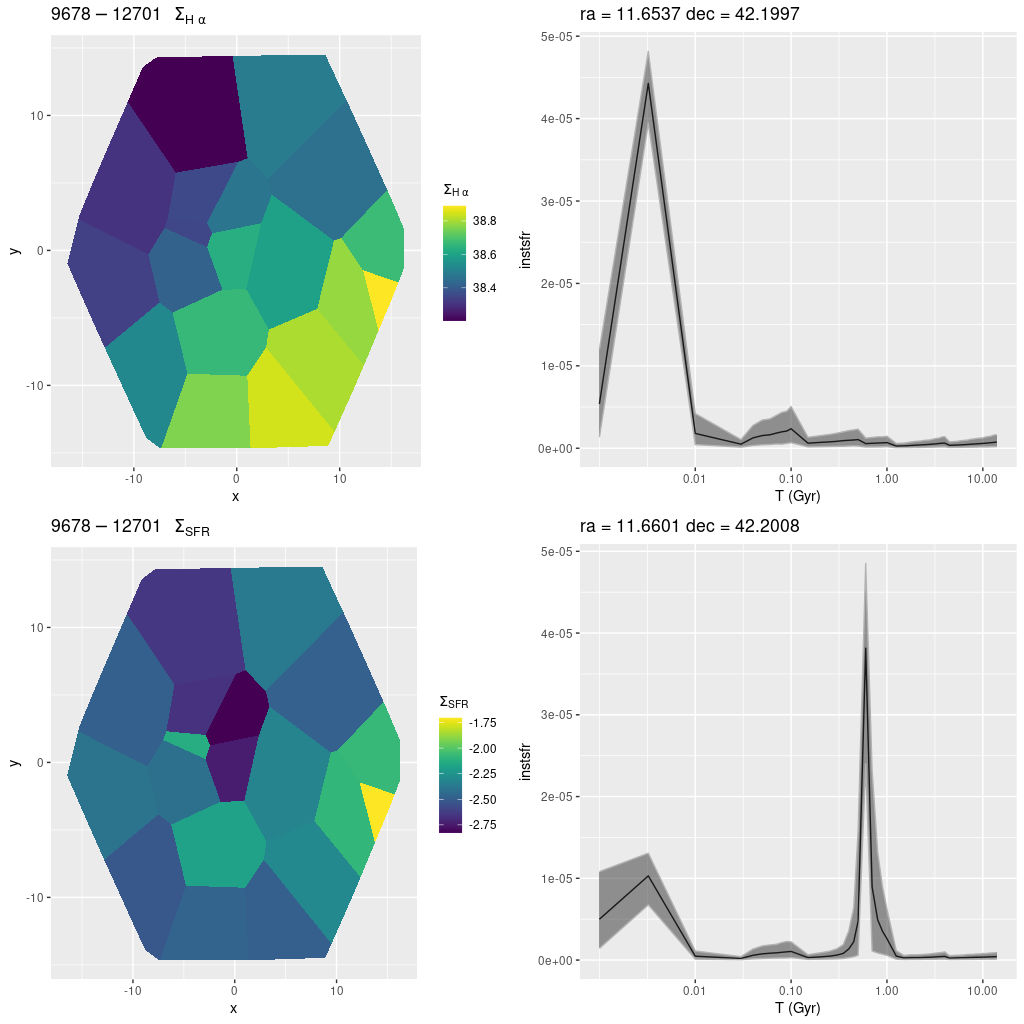
plateifu 9678-12701 (mangaid 52-25)
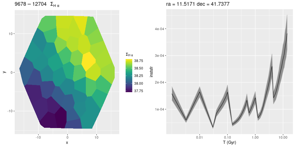
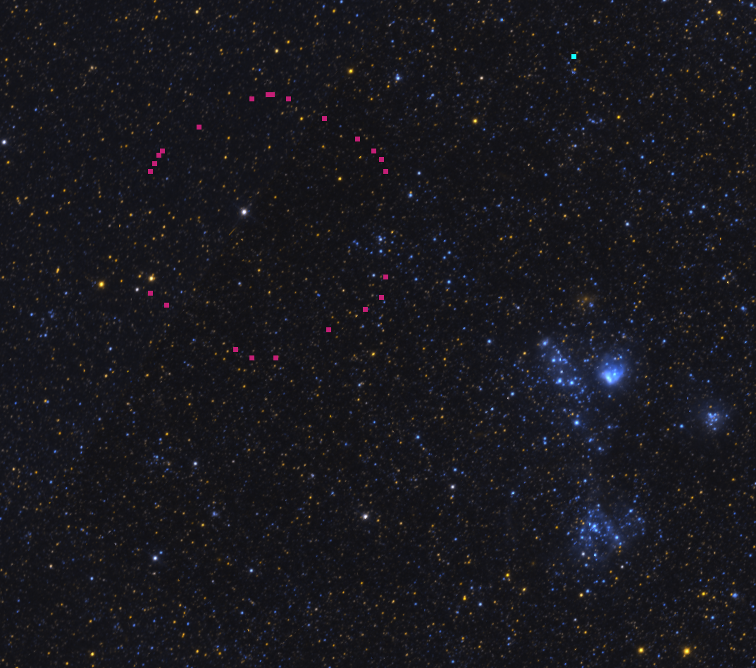
Finally, this is the outermost IFU in the program, located an estimated 15.7 kpc from the nucleus and very close to the major axis. Somewhat oddly it’s close to the most vigorously star forming region in this segment of the outer disk but offset by a little more than an IFU width. In fact in the Galex image it appears to be in a sort of notch with few UV bright sources.
MaNGA plateifu 9678-12701 (M31 outer disk)
Cutout from PHAT color image retrieved in Aladin.
No H II regions are cataloged within the IFU footprint but there is diffuse emission throughout with mostly starforming-like line ratios. The region with the highest modeled star formation rate is in the western corner of the IFU, where a number of blue stars can be seen in the PHAT color cutout. There is a single, somewhat isolated bright star near the center of the IFU. The SFH model for that region is in the lower right panel below. The model indicates a rather strong and short burst of star formation a little less than a Gyr ago. How much the model is influenced by the star is hard to say. The fit to the data is actually rather good. The star may be in the foreground: In Gaia DR3 (data retrieved through Aladin) its distance is listed as 2395 pc, which would obviously place it in the Galaxy. But that is based on estimates of its surface temperature and gravity rather than parallax, which is measured as negative and consistent with 0.
MaNGA plateifu 9678-12701 (M31 outer disk)
(TL) Hα luminosity density (uncorrected)
(BL) model star formation rate density
(TR) Star formation history for region with highest SFR density
(BR) SFH for a region with a bright starMaNGA plateifu 9678-12701 (M31 outer disk)
posterior predictive fit to the spectrum of a region with a bright star
After looking through all the data again I have to say I’m puzzled by some of the choices of IFU locations. All but 5 are in or very close to spiral features visible in Galex, but most are offset by as little as an IFU width from regions with more star forming activity. Even plateifu 9678-12703, which is very close to the most active starforming region in the PHAT coverage area, only captures the edge of a series of bright H II regions.
Overall I think the SFH models are successful with some caveats. Areas associated with bright Hα emission are generally showing increasing recent star formation rates reasonably consistent with the level of emission. It’s interesting that there are often nearby regions (separations ~10 pc or so) that have recently peaked but with high 100 Myr averaged SFR. This suggests we can actually see propagation of star formation over short distances and time scales.
A big concern is the effect of sampling small stellar mass regions, and in particular the effect of exceptionally luminous stars on model results. I plan to address this in a follow-up sometime soon.
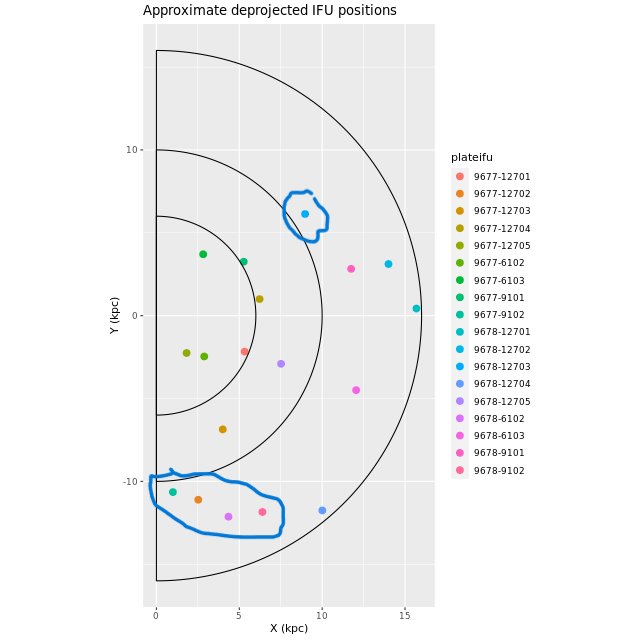
Before I get into details of the individual IFUs here is the result of a little exercise I did to estimate the deprojected positions of the IFU centers using the canonical values of 77° for the inclination and 38° for the major axis position angle, and applying the coordinate conversions I outlined way back in this post with slight modifications. These are fairly rough estimates since Andromeda’s disk is apparently warped and rather thick, but this may help give some perspective on relative positions in the plane of the galaxy. For reference I’ve drawn semcircles at 6, 10, and 16 kpc, and circled the IFUs that I had placed in the 10 kpc ring. Two of the IFUs — plateifus 9678-6102 and 9678-9102 — now appear to be at or beyond its outer edge at radii of 12.9 and 13.5 kpc, while plateifu 9678-9101 which I had assigned to the outer desk is a bit closer at 12.1 kpc. But, no matter. I will discuss them in the same order as I presented the IFU wide star formation histories several posts ago.
Approximate deprojected coordinates of M31 MaNGA IFUs. Coordinates are in kiloparsecs relative to the galaxy center, with the X axis parallel to the major axis and increasing to the northeast.
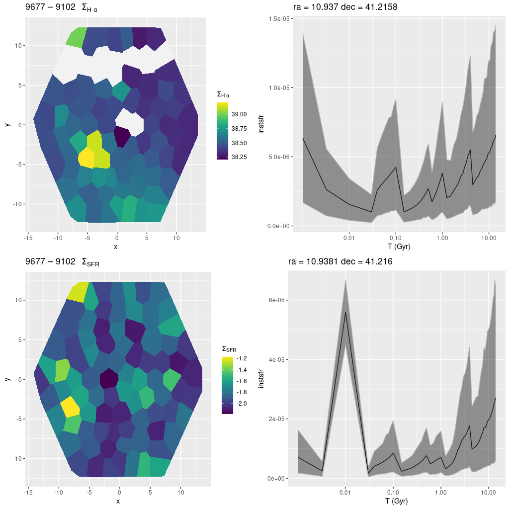
plateifu 9677-9102 (mangaid 52-1)
This is already a recurring theme. There is a single cataloged H II region within the IFU footprint that coincides with the highest (uncorrected) Hα luminosity density bin below. The bin with the highest (100 Myr) SFR density is displaced by several parsecs to the northeast. The first region has an increasing star formation rate over the last ~30 Myr, while the second shows a sharp peak and rapid decline over the last 10 Myr. If the models are remotely correct this is clear evidence for propagation of star formation over short distances.
plateifu 9677-9102 (M31 10 kpc ring).
(TL) Hα luminosity density.
(BL) SFR density (100 Myr average)
(TR) SFR history for the region with highest Hα density.
(BR) SFR history for the region with highest SFR density.
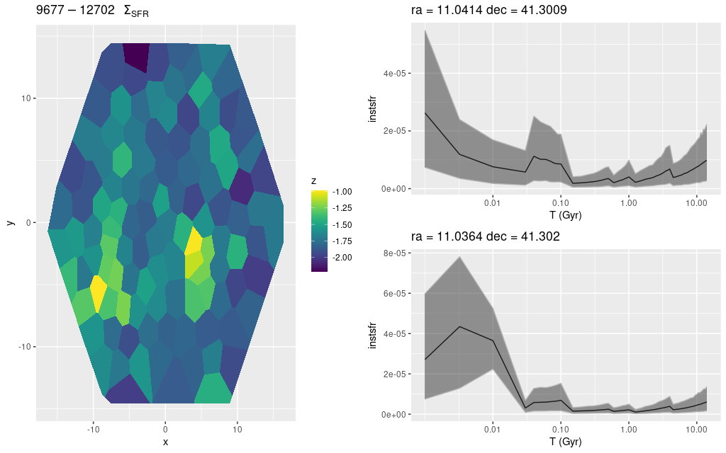
plateifu 9677-12702 (mangaid 52-7)
Despite being right in the middle of the 10 kpc ring there’s nothing very interesting in this IFU, with just a single cataloged red supergiant and a small and rather faint H II region that’s at or beyond the edge of the footprint. Only weak diffuse emission is seen in the MaNGA data. Nevertheless there are a few areas with evidence for recent star formation:
plateifu 9677-12702 (M31 10 kpc ring)
(L) map of SFR density
(R) star formation histories for 2 regions with higher than average SFR density.
I recently noticed that one of the imaging products available in Aladin is a color composite assembled from the PHAT F475W and F814W ACS/WFC observations. One thing these are good for is they give you a very rough idea of stellar temperatures. To my eyes at least stars appear orange, white, or blue. Bright blue stars must be young; bright orange ones are evolved (or reddened by dust perhaps) and might be young or old. Notice below that the two areas with relatively high star formation have a sprinkling of bright blue stars, while the bulk of the field contains predominantly orange ones.
The other optical wavelength imaging I look at comes from SDSS. Even though the imaging in this area is incomplete and the processing leaves something to be desired it does have the virtue that Hα is, at low redshift, in the r filter, which forms the green channel in their images. M31 H II regions then are identifiable by their green color. Also, red supergiants look distinctly red since their brightness is still increasing into the near IR.
plateifu 9677-12702 (M31 10 kpc ring)
Cutout of PHAT color composite taken from Aladin
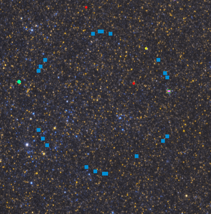
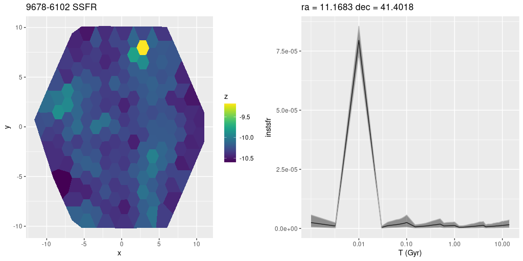
plateifu 9678-6102 (mangaid 52-20)
This lies on the outer edge of the 10 kpc ring, some distance from UV bright sources and H II regions. There is one cataloged planetary nebula and that shows up in my modeling as a region with “AGN” like emission line ratios. One fiber has a much higher modeled specific star formation rate than its surroundings. A map of SSFR and star formation history for that region are shown below. There are bright red and yellow stars in the region which might be (uncatalogued?) red supergiants.
MaNGA plateifu 9678-6102 (M31 10 kpc ring)
(L) map of model specific star formation rate
(R) star formation history for the region with highest SSFR
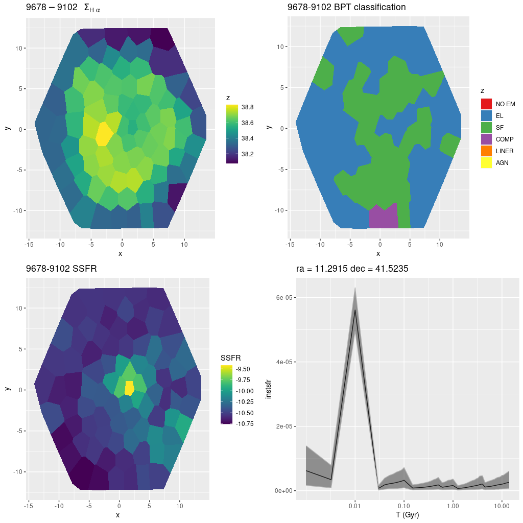
9678-9102 (mangaid 52-18)
This is the final IFU on the eastern side of the 10 kpc ring. Once again it lies at the outer edge, well away from active star forming regions. There is weak emission throughout, with star forming line ratios through much of the IFU footprint despite the lack of evident star forming regions. There’s some unresolved UV emission in the GALEX color image that roughly corresponds in location to the area of brighter Hα.
The region with the greatest recent star formation has some fairly bright blue and yellow stars in the PHAT color image
plateifu 9678-9102 (M31 10 kpc ring)
(TL) Hα luminosity density
(TR) BPT classiication by [N II]/Hα vs {O III]]/Hβ diagnostic
(BL) 100Myr average specific star formation rate
(BR) model star formation history for the region with highest SSFR
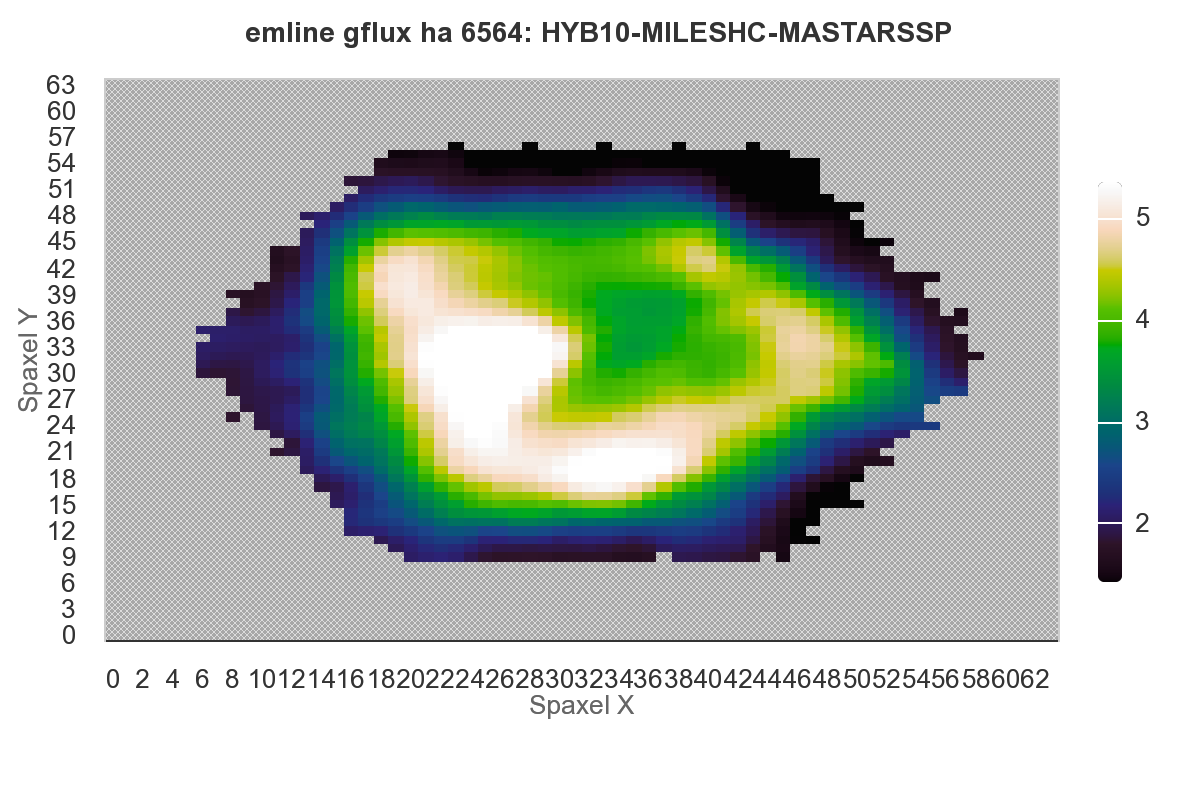
By the way I do check observational quantities in my models against the SDSS product Marvin now and then. Here’s their rendering of the Hα flux:
Qualitatively at least the agreement is excellent. I’d have to check if their fluxes are consistent with my log-luminosities.
plateifu 9678-12703 (mangaid 52-23)
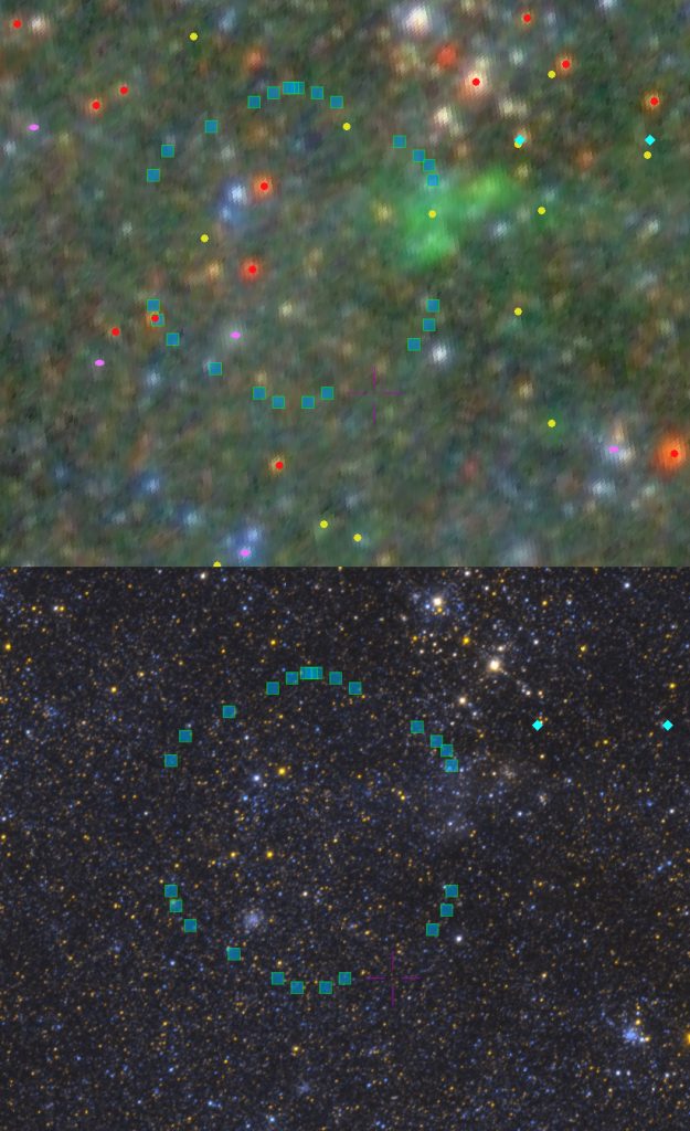
Finally we get to the most interesting IFU in the project, plateifu 9678-12703, which lies very close to the region with the highest recent star formation in the northeastern half of the galaxy. It also appears to coincide in position with one of the regions that Lewis et al. (2015) highlighted (their Figure 2). As can be seen in the Aladin cutouts (from SDSS and PHAT color images) below there are several young stellar objects within and near the IFU footprint: at least two red supergiants (which are a problem); 3 catalogued H II regions, one of which is bright and extended; some OB associations that are centered outside the footprint; and one open star cluster. There are a number of bright blue stars scattered throughout as can be seen in the color PHAT image.
plateifu 9678-12703 (M31 10 kpc ring)
Symbols: yellow circle: H II region
red circle: red supergiant
purple oval: star cluster
blue rhombus: OB association
blue squares: IFU outline
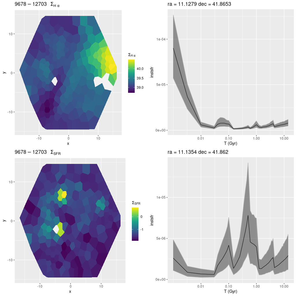
Plotted below are maps of Hα luminosity density and model star formation rate density, along with model star formation histories for two regions. The first is for the bins in the brightest part of the H II region along the western edge of the IFU. The second is for two bins at the position of a cataloged open cluster (Johnson et al. 2016) that’s fairly obvious in the PHAT cutout. The cataloged (log) age of the cluster is 8.4-0.1+0.3 with a mass around 104 M☉. The peak star formation rate in the model history below (bottom right) is at about 500 Myr lookback time with several hundred Myr of enhanced star formation, so this is pretty good agreement.
plateifu 9678-12703 (M31 10 kpc ring)
(TL) Hα luminosity density (uncorrected)
(BL) model star formation rate density
(TR) star formation history for areas with highest Hα luminosity.
(BR) SFH for a region covering a cataloged open cluster
When I did my initial fitting runs on this IFU I noticed one fit that was rather poor which I attributed to a foreground star, and therefore I masked it for subsequent analysis. It turned out though the culprit was not a foreground star but instead a local red supergiant that’s been cataloged (for example) by Ren et al. (2021). Their catalog lists its G band magnitude from Gaia DR2 as 19.1 which makes its absolute magnitude around -5.3, a reasonable value for its presumed spectral type.
This raises an issue that’s fairly well known. Simple stellar population models assume the age zero main sequence is fully occupied according to a well defined initial mass function. This is a fairly innocuous assumption (although the choice of IMF is not) when we’re sampling ~billion solar mass regions, but it’s not so innocuous for cluster size agglomerations, which is what we’re sampling here1the typical binned region has a present day stellar mass around 104 M☉ per my models. The particular problem here is that a single red supergiant is making a significant contribution to the spectrum in the red, and that could be biasing the model SFH in as yet unexplored ways.
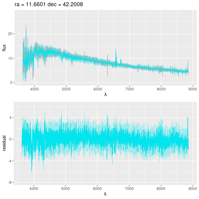
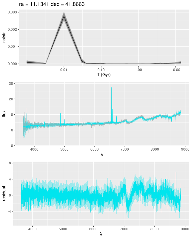
The bin at the position of the other bright supergiant in the footprint was analyzed, so lets take a quick look. In the top pane below is the model star formation history, and in the two below the (posterior predictive) fit to the data and the residuals from same. The fit doesn’t look so bad except for a region around 7200 Å, which often seems to be a problem with EMILES spectra.
Superficially the model star formation history looks not implausible, and similar to others I’ve shown. The presence of an evolved star indicates a stellar age in the right general range, as does the relative lack of H II emission. Despite the strength of the burst it adds only about 7% to the present day stellar mass, with as elsewhere the majority of the stellar mass was in place by 8 Gyr ago (per the model, as always).
But, there’s at least one indicator of a problem: the modeled optical depth of attenuation is extraordinarily high at τV ≈ 4.4, compared to the optical depth estimated from the Balmer decrement of τVbd = 1.47 ± 0.23. I plan to discuss this in more detail in a future post, but for now I’m moving on.
plateifu 9678-12703 (M31 10 kpc ring)
model star formation history for a region with high recent SFR
plateifu 9678-9101 (mangaid 52-26)
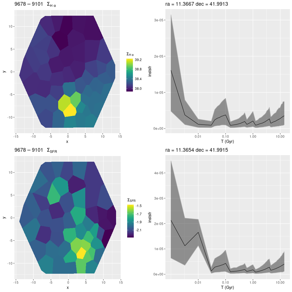
As mentioned at the top this appears to be in a spur off the 10 kpc ring. There is just one cataloged H II region within the footprint that appears to be compact. Just to the west there is a sprinkling of bright blue stars and an unresolved blob in the Galex color image. The H II region is evident in the map below. Once again the regions with the highest Hα luminosity and highest (100 Myr averaged) star formation rate are slightly offset from each other. The model star formation histories are very similar though.
plateifu 9678-9101 (M31 10 kpc ring)
(TL) Hα luminosity density (uncorrected)
(BL) model star formation rate density
(TR) star formation history for area with highest Hα luminosity.
(BR) SFH for area with highest recent star formation rate
I’m going to stop for now and cover the last 4 outer disk IFUs in (probably) the next post.