star formation history modeling – Page 3

2023-03-232023-03-23

The MaNGA M31 ancillary program – comparing star formation history models

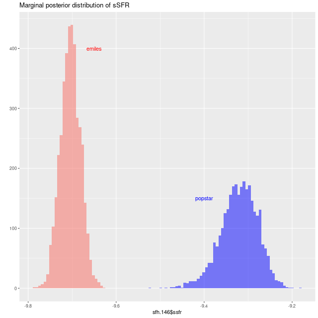
In this post I’m going to compare IFU wide star formation histories from my models to those of Williams et al. (2017) in the nearest 83″ by 83″ PHAT tile to each MaNGA IFU in the study. I picked the Williams paper for comparison mostly because it’s possible to! They give a complete tabulation of model results for all regions and all 4 sets of isochrones that they used, and these are available through the Vizier service. Specifically I used their Table 2, which provides star formation rate densities summed over all metallicities. Since the SSP model spectra I use are based on BaSTI isochrones I initially compared to their BaSTI based models. One problem with the Williams comparison is the authors had a very wide youngest time bin of 300 Myr, which is where my models should generally have the highest precision (I make no strong claims about accuracy). It would be nice to do a similar comparison to the earlier companion paper on recent star formation by Lewis et al., which gives a much finer grained view of the last ~half Gyr, but unfortunately there is no published tabulation of their results.

At the other end of the timeline the oldest bin is also very wide, from 8 to 14 Gyr lookback time. This isn’t a surprise: the limits for reliable photometry of individual stars were rather shallow, no fainter than m = 28 or M_g ≈ 3.6 according to Lewis. This is brighter than the main sequence turnoff at 8 Gyr, so any information about the truly ancient star formation history is coming from giant branch stars which have very similar evolutionary tracks at old ages¹

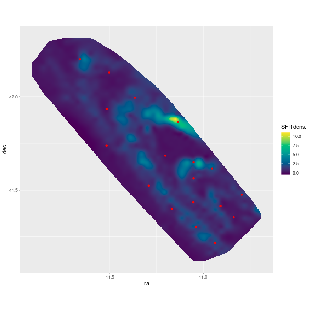
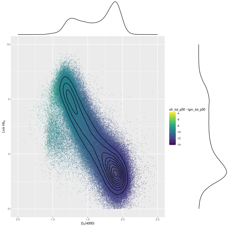
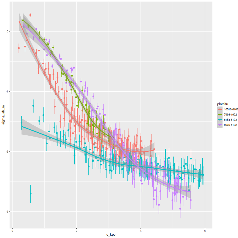
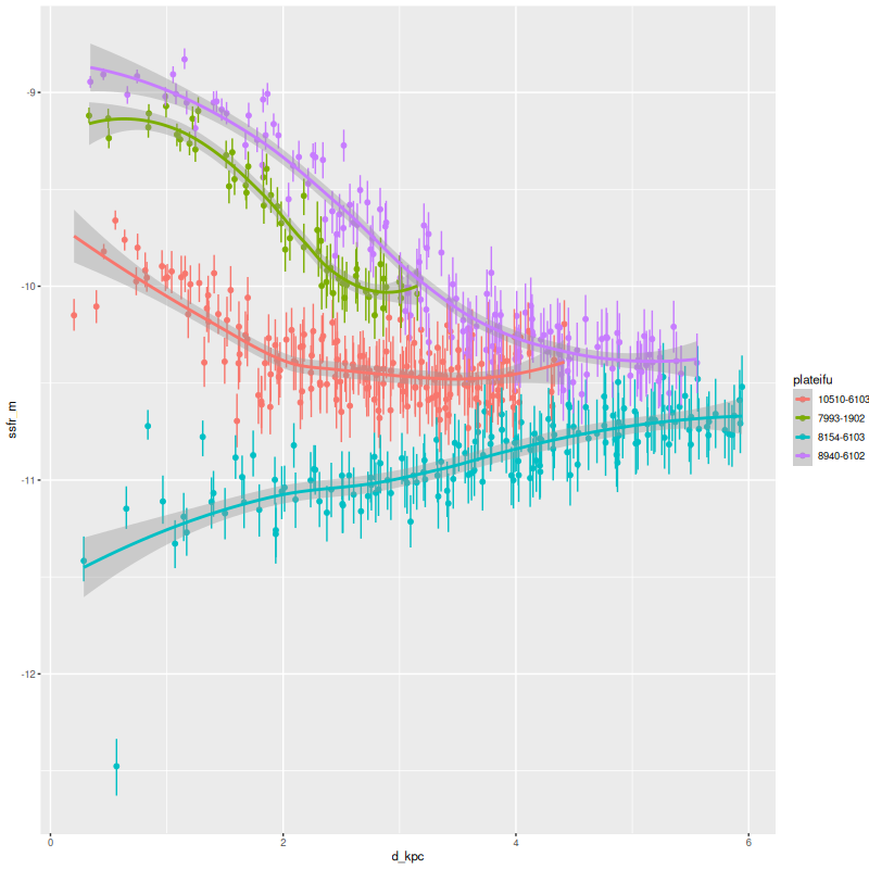
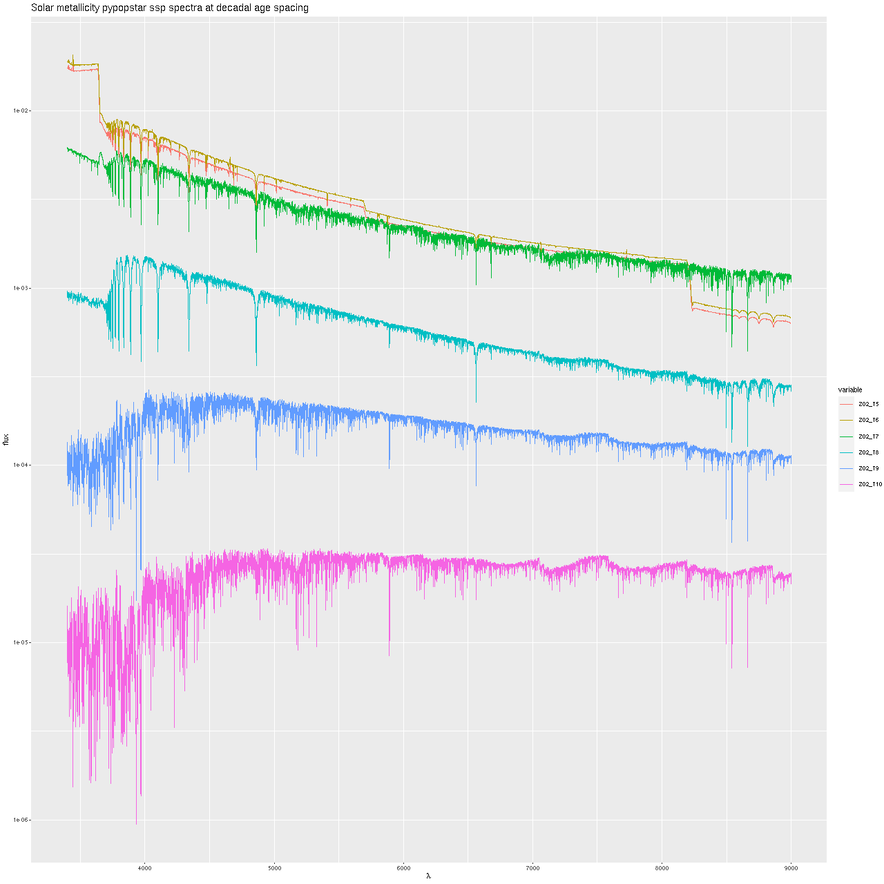
At the end of my last post I mentioned the necessity to correct densities for the rather large inclination of M31’s disk. It turns out though that I reproduce Williams’ Table 3 from their Table 2 if the densities are uncorrected. Their tabulated SFR densities are in units of 10^-4 M_☉arcmin^-2/year. One arcminute at their adopted M31 distance is about 0.227 kpc, so to convert to star formation rates per kpc² the values in table 2 are multiplied by 19.8 × 10^-4. From my models I sum the star formation rates over all modeled spectra in each IFU and divide by the total area in fibers, with each fiber covering a projected area of 42.78 pc². Note that I do not try to analyze a single composite spectrum summed over the entire IFU since dust attenuation is quite patchy.

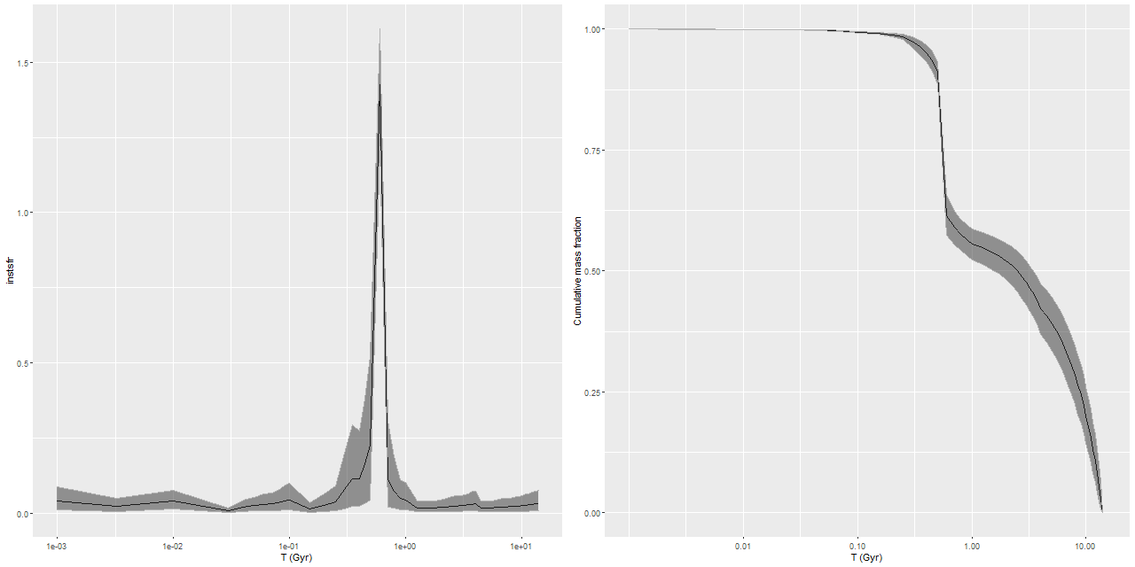
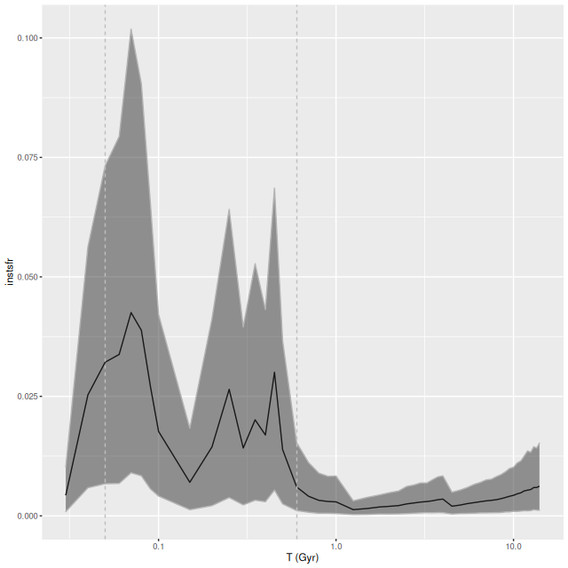
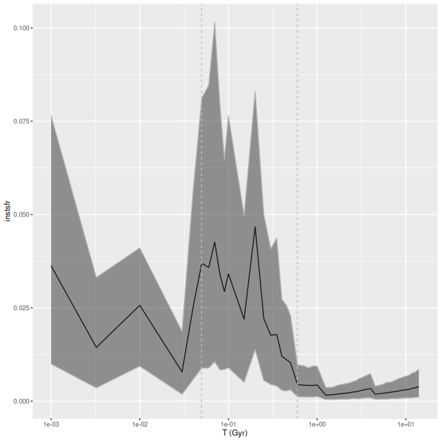
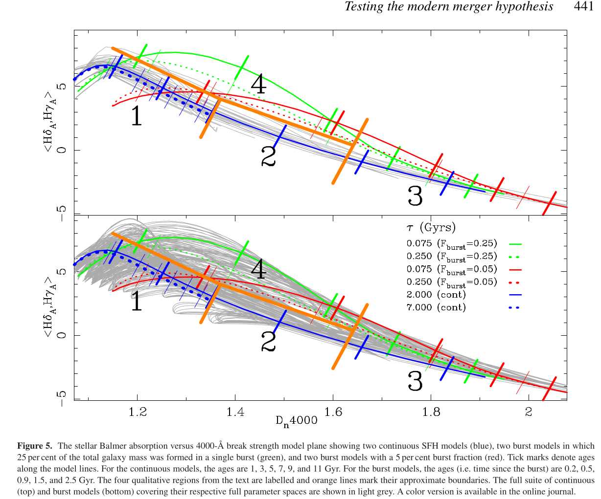
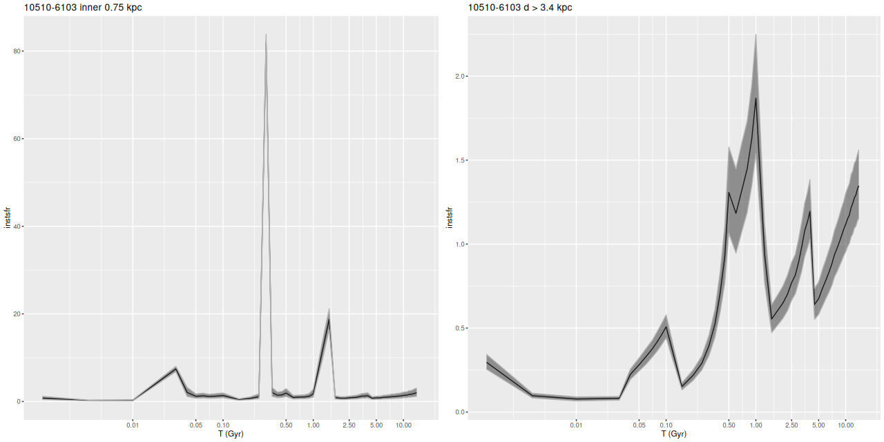
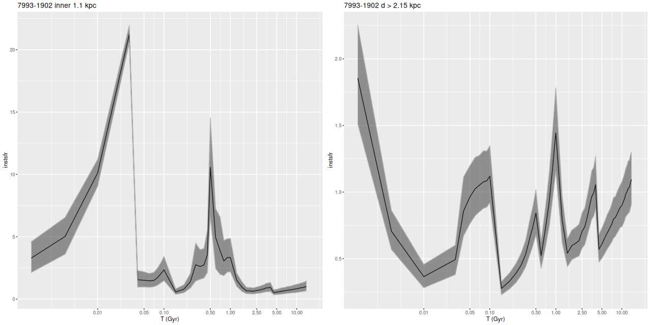
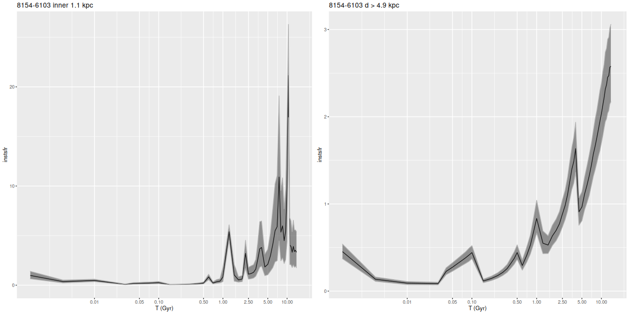
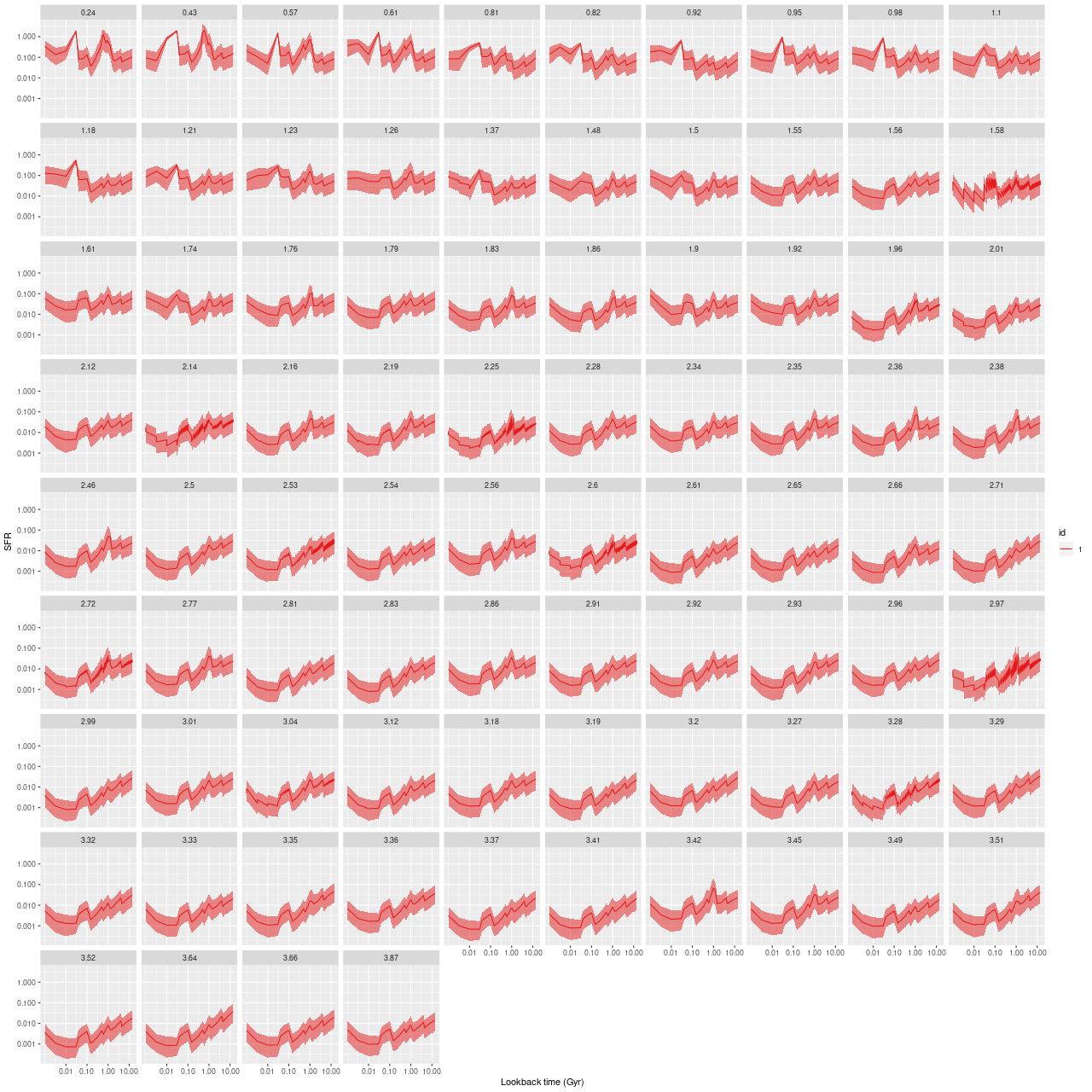
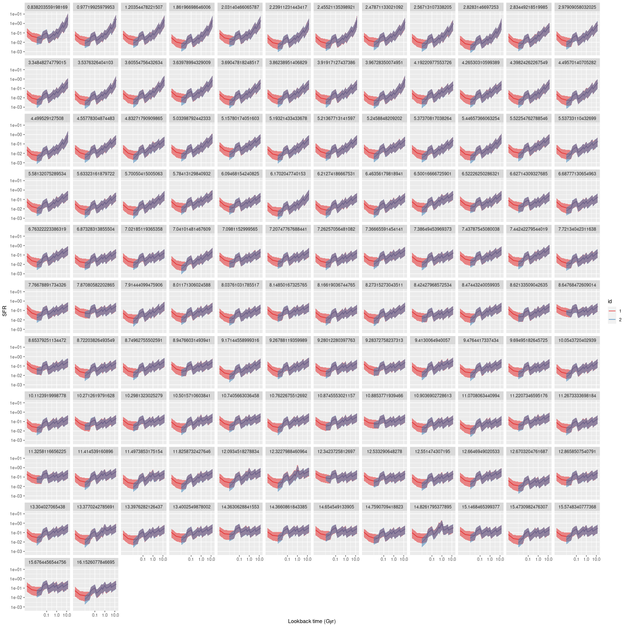
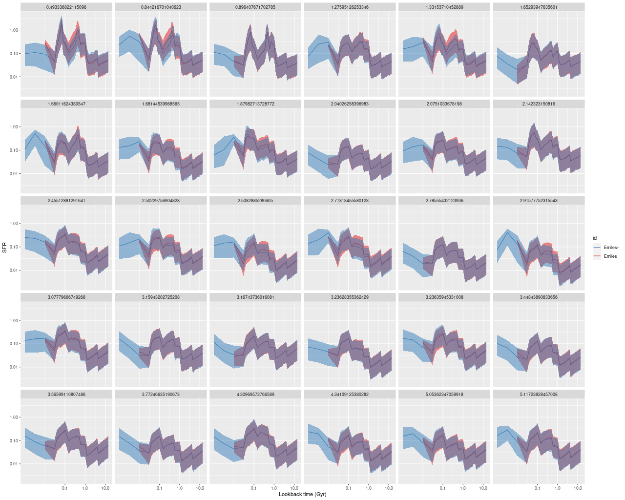
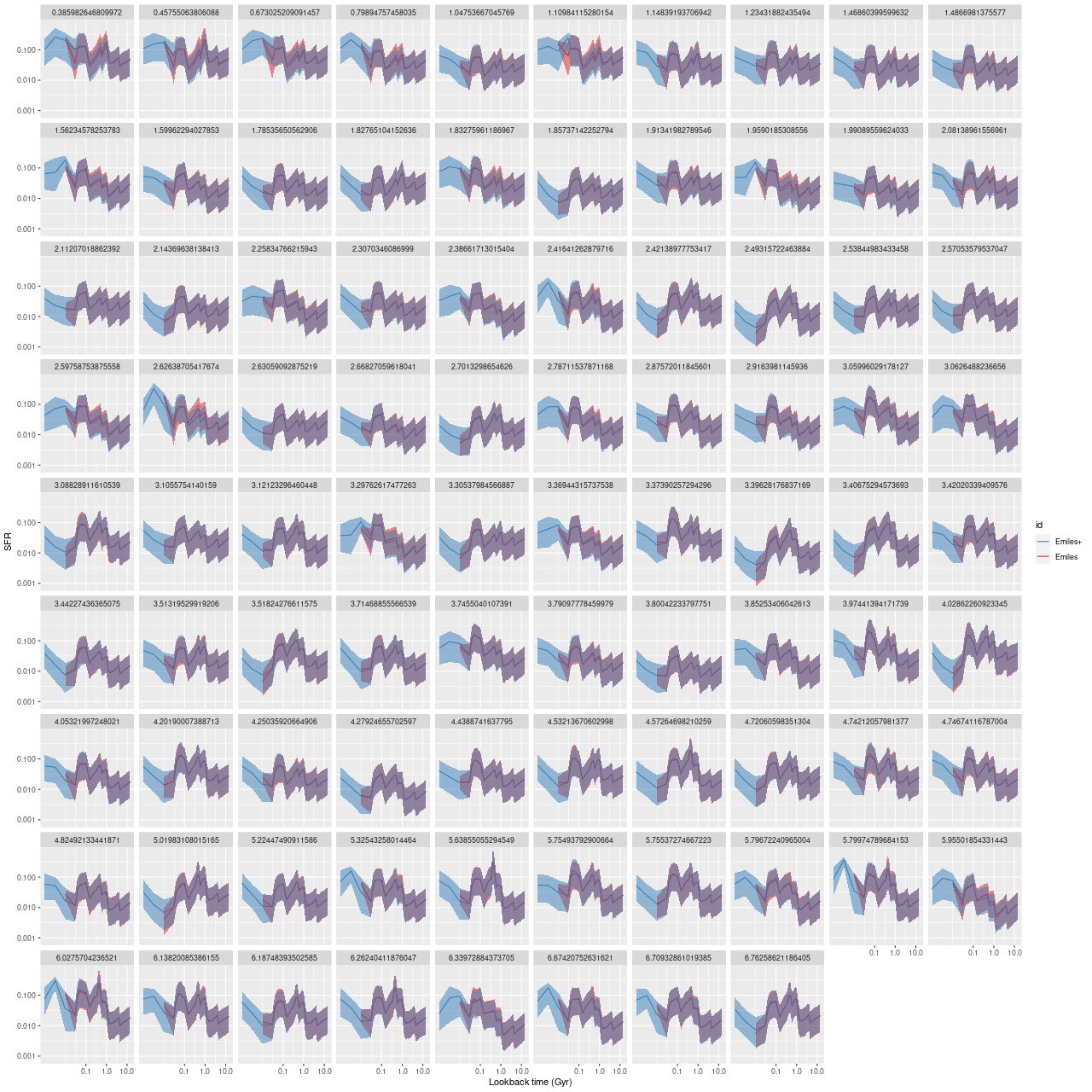
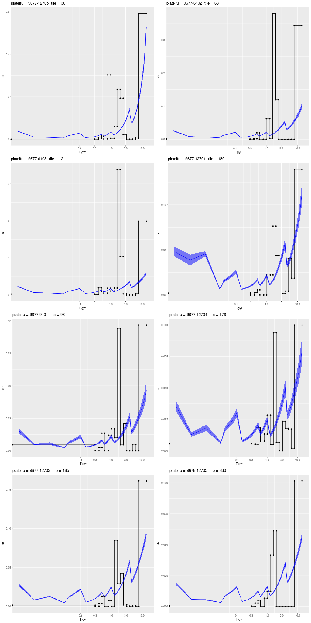
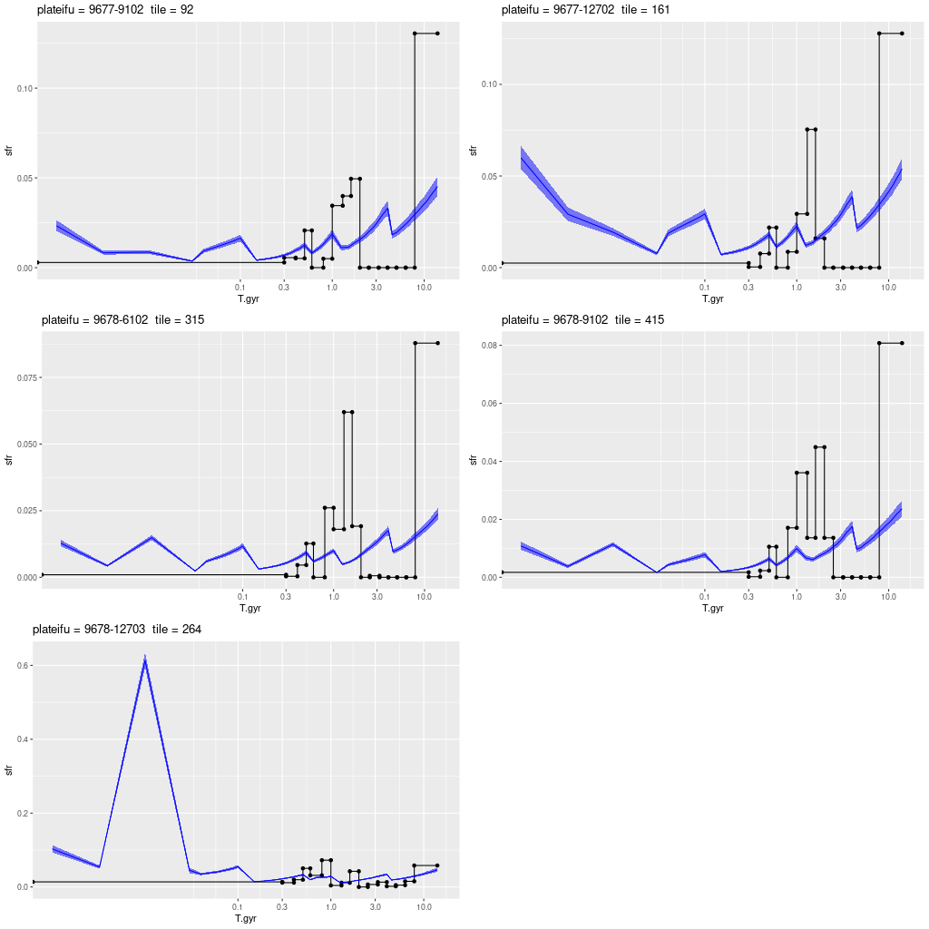
The graphs below overlay my modeled star formation rate densities on those of Williams in the tile with the nearest center to that of each IFU. The ribbons indicate the nominal 95% credible limits of SFR. These are certainly wildly optimistic. Table 2 of the paper includes uncertainty estimates, which I chose not to include. SFR densities are linearly scaled with different limits for each plot. The time scale is logarithmic. Something in between linear and logarithmic would seem more appropriate since this perhaps gives too much space to very recent times, but I haven’t found a suitable scaling.

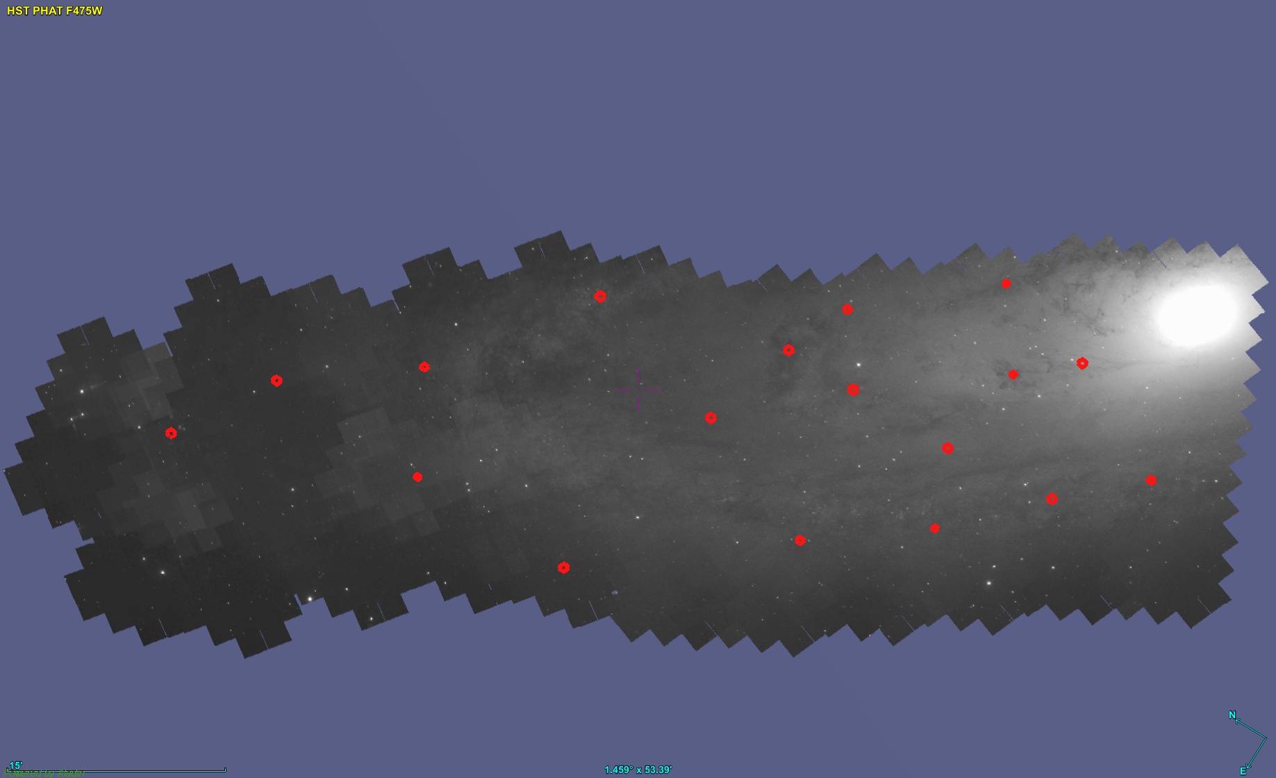
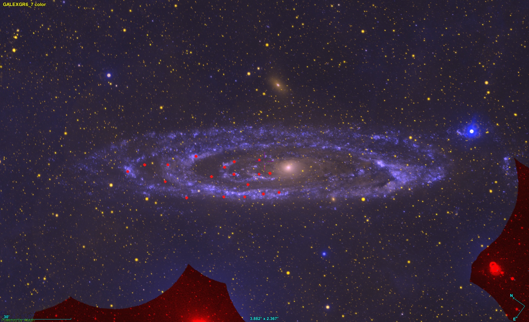
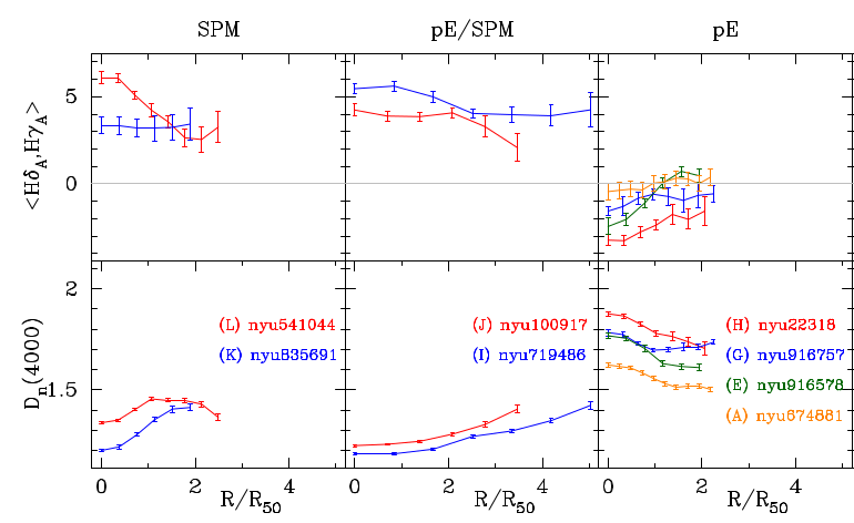
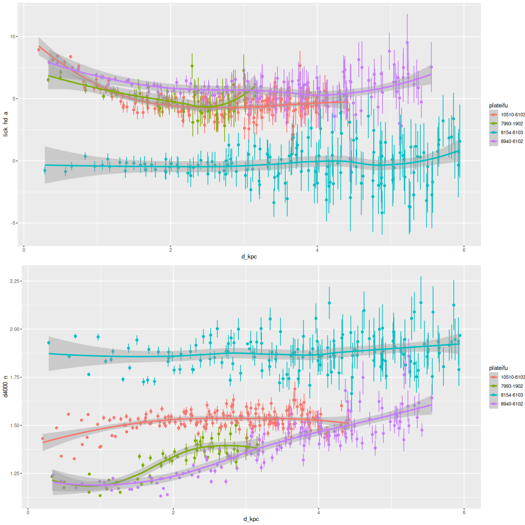
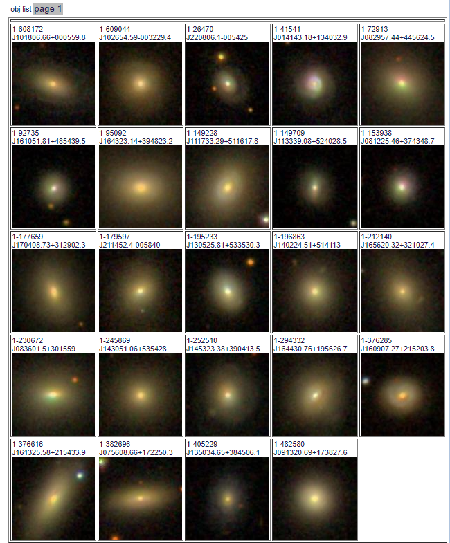
These are ordered into three groups by location: the inner disk which is everything inside the 10 kpc ring, the 10 kpc ring, and the outer disk which is everything outside the 10 kpc ring. There’s some ambiguity about the locations of the plateifu’s 9678-9101 and 9678-12704. The first of these is about 12 kpc from the nucleus in what could be either a wide section of the 10 kpc ring or a separate structure. 9678-12704 appears in projection to be just outside the 10 kpc ring but it may be considerably farther out in a segment of spiral arm at ~15 kpc.

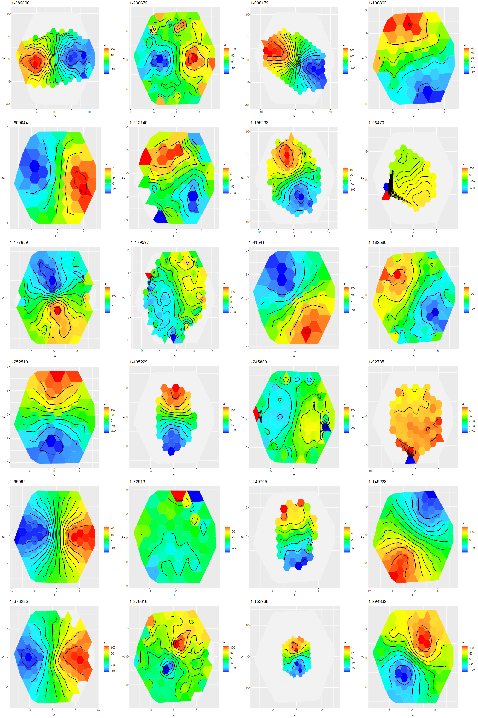
Commentary will continue after the graphs. I will discuss the individual IFU’s in more detail in later post(s).

Inner Disk

10 Kpc ring

sfh_10kpc — M31 MaNGA ancillary program – my star formation history models summed over each IFU compared to nearest tile in Williams et al. (2017) with BaSTI isochrones. 10 kpc ring IFU’s.

Outer disk

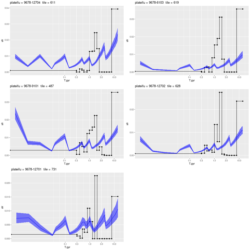
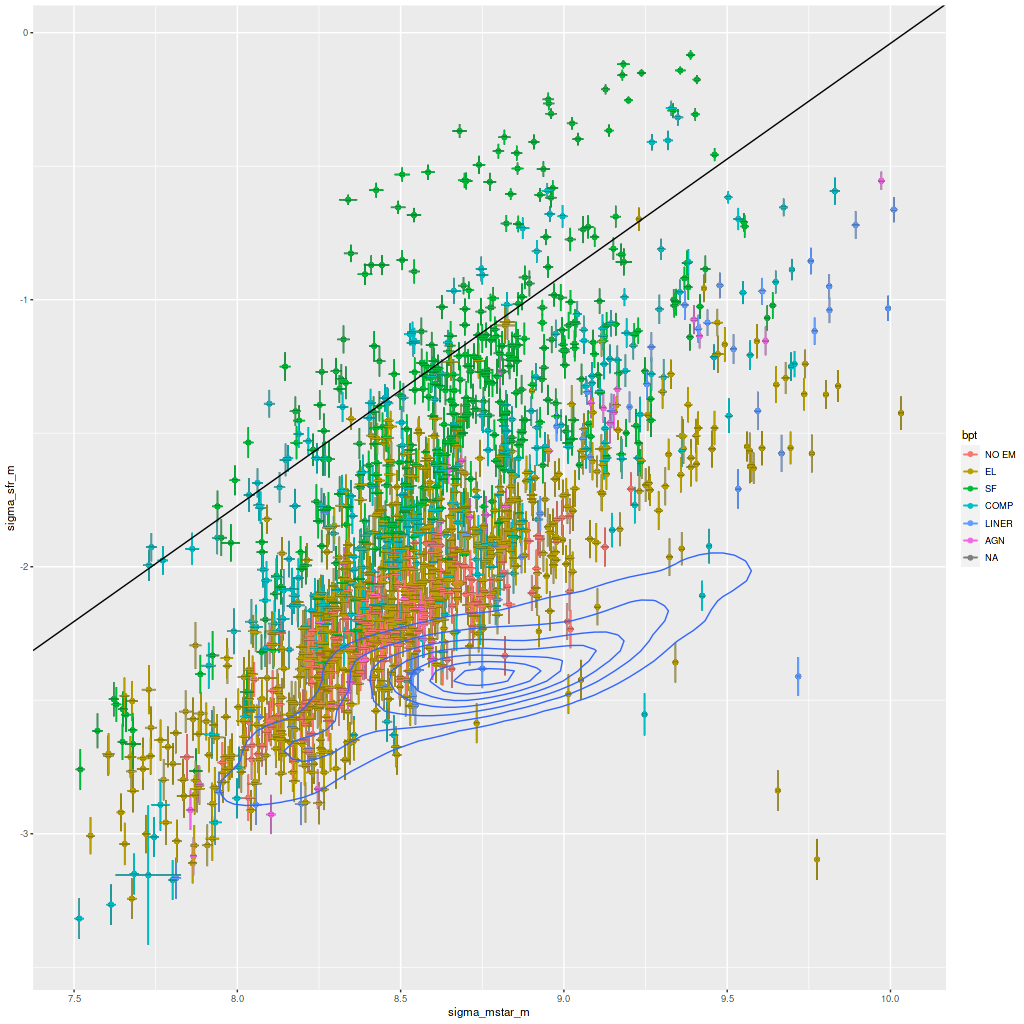
The first two things I noticed were that star formation in every region declines monotonically from very early times to at least 4 Gyr ago. It also starts out lower than in the PHAT team’s models. Because of this early time mass deficit all of my models have smaller current day stellar mass densities by varying amounts. I don’t really have a pat explanation for this. Some authors have posited a “dazzle effect”² where recent star formation obscures the contribution of old populations. It’s certainly likely that this occurs, but if these Bayesian models are behaving as I hoped this lack of information should manifest as larger uncertainties rather than a systematic bias. Well, my hope could be wrong. On the other hand I don’t see strong evidence in these models for such an effect. From my eyeball analysis I don’t see an obvious correlation between present day star formation and the size of the early time deficit.

Another possibility is a systematic difference in the amount or shape of attenuation between my models and theirs. There is another well known “degeneracy” between stellar age and attenuation in SFH modeling, but I haven’t yet investigated whether this could be occurring here.

The PHAT models have a very long interval from 8 to ~2-3 Gyr ago with very little star formation. Some authors find evidence for a large increase from about 2-4 Gyr which is usually attributed to a merger or perhaps close encounter with M33. This isn’t seen in the BaSTI based models but there is a large more recent burst from about 1-2 Gyr lookback time. My models see neither a cessation of star formation nor a particularly large burst at intermediate ages. As I’ve noted before my models “want” to have smoothly time varying light³ contributions and this might make a modest burst at moderately large ages difficult to discern. Another confounding factor arises from the abrupt changes in age intervals (at 0.1, 0.5, 1, and 4 Gyr) which results in the sawtooth pattern in SFR that’s obvious in every plot above.

At ages younger than 1 Gyr there’s generally good agreement about the course of star formation up until the youngest age bin of width 300Myr in the PHAT models. My models have anywhere from slightly to dramatically higher SFR densities averaged over the most recent age bin. I suspect this is because many of the IFU positions were chosen to be in regions with active star formation. In particular the plateifu 9678-12703 (mangaid 52-23) is very close to the region in the 10 kpc ring with the highest density of ongoing star formation in the northern half of the disk.

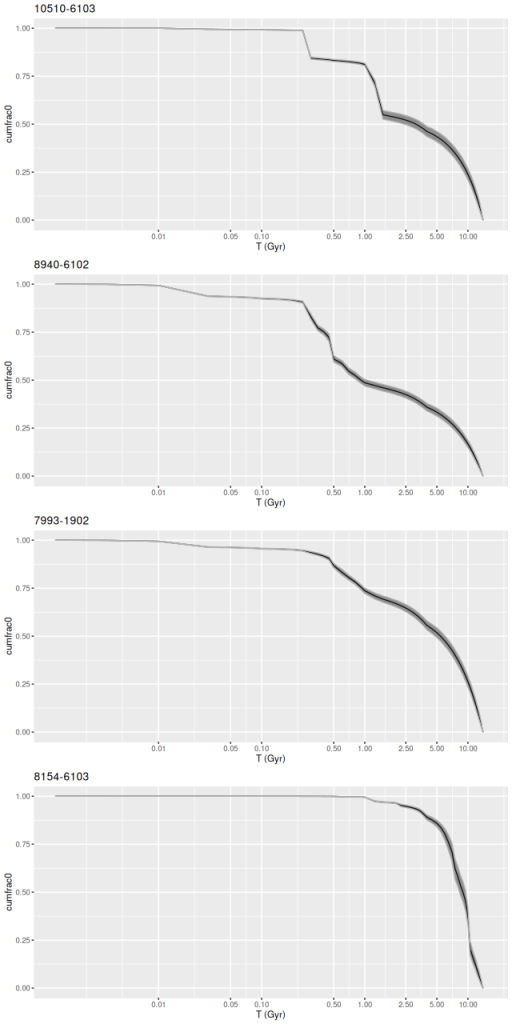
I plan to discuss the individual IFUs in more detail in a later post. Below the fold are some more graphics: mass growth histories and SFR densities compared to the PADOVA isochrone based models.

2023-02-28

The MaNGA M31 ancillary program – preliminaries

One of the ancillary programs (with principal investigator Julianne Dalcanton) in the final MaNGA release targeted 18 fields in the disk of the Andromeda galaxy M31. The targets were selected from within the footprint of the “Panchromatic Hubble Andromeda Treasury,” aka PHAT¹, also with PI Dalcanton. The initial PHAT survey description was in Dalcanton et al. (2012) and was followed by a lengthy series of papers. Especially relevant for this discussion are two papers describing estimates of the recent and ancient star formation histories of the disk outside the area dominated by bulge light: Lewis et al. (2015), “The Panchromatic Hubble Andromeda Treasury. XI. The Spatially Resolved Recent Star Formation History of M31” and Williams et al. (2017), “PHAT. XIX. The Ancient Star Formation History of the M31 Disk.” For reference here is a mosaic of HST images in the F475W filter with the IFU locations overlaid:

m31manga_phathst — Mosaic of HST F475W images of PHAT study region with M31 MaNGA IFU positions overlaid

Zooming out to show the whole disk here they are overlaid on a false color FUV+NUV image from GALEX, which gives a pretty good picture of where stars are actually forming:

m31manga_galex — GALEX false color NUV+FUV image of M31 with MaNGA IFU positions overlaid – screencap from Aladin

This data set provides an excellent opportunity to compare my SFH modeling code to a completely different, more direct, method of inferring star formation histories namely counting resolved stars in color magnitude diagrams. I recently completed model runs for all 18 IFU’s with the same Voronoi binning of stacked RSS spectra, the same modeling code and SSP model spectra as I’ve used for a while now.

There’s no redshift listed in the DRP catalog; NED gives a heliocentric redshift of -0.001, but for purposes of calculating intrinsic quantities I need the “Hubble flow” redshift. I adopted a distance of 761 (± 11) kpc or distance modulus of (m-M)₀ = 24.407 from Li et al. (2021), which is the most recent and according to the authors most precise determination to date. With my adopted Hubble constant of H₀ = 70 km/sec/Mpc this makes the Hubble flow recession velocity 53.27 km/sec or z_dist = 0.0001777. The angular scale is 3.69 pc/arc-second. This distance estimate is a few percent smaller than the PHAT team authors and most other recent literature I reviewed, but fortunately most other sources of uncertainty are much larger.

An issue I noticed early on was the modelled values of the optical depth of attenuation were right at 0 for almost all spectra with only a few much larger exceptions. A quick check of the metadata showed that the values adopted for the foreground galactic extinction almost certainly were taken from the SFD dust maps which faithfully capture the intrinsic dust content of M31 albeit at rather low resolution. These hugely overestimate the actual foreground galactic extinction and that has multiple undesirable consequences. So, I assigned a single extinction value of E(B-V) = 0.055 to all IFU’s, consistent with the NED value of A_V = 0.17 mag. The preliminary runs were redone with the newly adopted extinction value.

After binning to a minimum mean SNR of 5 there were 2,624 spectra in the 18 IFUs, of which I ran models for 2,621. Three spectra had apparent foreground stars, although one of those might actually be a red supergiant in M31. The fibers are basically sampling star cluster size and stellar mass regions so a single extremely luminous star could potentially affect a spectrum.

I’m only going to show a few summary results for the entire sample in this post. My goal is to do a more detailed quantitative comparison to (at least) the SFH models of Wilson, for which there are extensive results tabulated. There are of course many catalogs of interesting objects within M31, and I plan to look at some of them.

First, here is a plot of the (100 Myr averaged) star formation rate density against stellar mass density, color coded by BPT diagnostic. The solid line is my estimate of the “spatially resolved star forming main sequence” based on a small sample of non-barred spiral galaxies. The dashed line is the estimate of Bluck et al. (2020), which I commented previously appears to mark approximately the location of the green valley at least with regard to my models. A striking feature of this plot is the apparent stratification into at least three distinct groups that can be interpreted as starforming, quiescently evolving, and passively evolving. I suspect this observed stratification is just the result of hand picking a small number of “interesting” regions. Most or perhaps all of the points in the passively evolving group are in the IFU closest to the bulge, while most of those along and above the SFMS lie near the most vigorously star forming regions in the PHAT footprint. Especially noteworthy are 5 outliers that are well above any others in the plot in terms of SFR density. These are all in the same IFU (plateifu 9678-12703) which is located within the largest star forming region in that quadrant of the “10 kpc ring.”

m31manga_sigmam_sigmasfr — 100 Myr average star formation rate density vs. stellar mass density for 2621 binned spectra in M31 disk. Solid and dashed lines are my and Bluck’s central estimates of the “spatially resolved star forming main sequence.

Next are plots of star formation rate density against Hα luminosity density. The left panel is for all spectra color coded by BPT diagnostic, with Hα adjusted by the modeled amount of stellar attenuation. The right panel shows regions with star forming BPT diagnostics only, with Hα corrected by the observed Balmer decrement. The solid line in both panels is Calzetti’s calibration of the Hα – SFR relationship. The relationships plotted here are consistent with what I’ve seen in other MaNGA samples and with published values, which is encouraging.

m31manga_sigmaha_sigmasfr — Star formation rate density vs. Hα luminosity density for 2621 binned spectra in M31 disk. (L) Emission corrected for modeled stellar attenuation. (R) For regions with star forming emission line ratios only: emission corrected from estimated Balmer decrement.

The obvious point of comparison to my models are the detailed star formation histories in the two PHAT papers mentioned at the top. Unfortunately there is no detailed tabulation of model results in the paper by Lewis et al. The paper by Williams et al. has extensive tables, but there are still a few obstacles to detailed comparisons which I will discuss next time.

A few more items from my handwritten notes that I want to get in pixels. I have never previously tried to correct surface densities for inclination in disk galaxies, but for comparison purposes and because of the large inclination of M31’s disk I need to do so here. I adopted an inclination angle of 77°, so a 1″ radius fiber covers a 3.69 x 16.4 pc (semi major and minor axes) elliptical region, or 190 pc². Densities need to be adjusted downward by a factor 4.45 or -0.648 dex².

In order to achieve 100% coverage of the IFU footprints the exposures were dithered to three different positions with overlapping fiber positions. Comparing the area in fibers to the area in spaxels in the cubes the overfilling factor averages 0.217 dex or 65%. The total area in all cubes is 10,731 arcsec², or a deprojected area of 0.65 kpc². The most distant IFU from the nucleus is at a projected radius of about 16 kpc. A simple extrapolation to the ≈800 kpc² area of the disk within that radius is probably unsafe.

One final map to anticipate the next post(s). Wilson provides tables of model star formation rates for 16 age bins, 826 regions, and 4 different sources of isochrones including the same BASTI isochrones I use. The complete data set is available through Vizier. In the plot below I created a map of the recent star formation rate density interpolated to nominal 10″ resolution from their Table 2 models with BASTI isochrones. This should be compared to their Figure 16 (they use logarithmic scaling).

m31manga_wilsonsfr — Current (300 Myr average) star formation rate density in the PHAT footprint per models of Wilson et al. (2017) with positions of MaNGA IFUs overlaid.

2022-09-28

A little more on the “burst age – burst mass degeneracy”

I just have a quick comment about my last two subjects. I mentioned both of them have exceptionally strong Balmer absorption as measured by the Lick index Hδ_A. They also have similar 4000Å break strengths:

IC 0976: D_n4000 = 1.308±0.005, Hδ_A = 8.05±0.31
MCG +07-33-040: D_n4000 = 1.153±0.009, Hδ_A = 8.06±0.41

For context here’s a variation of the same plot I’ve shown several times of the MPA-JHU measurements for a large sample of SDSS galaxy spectra with their locations overlaid:

hd_d4000_2psb — D_n4000 – Hδ of SDSS spectra of post-starburst galaxies IC 976 and MCG +07-33-040 overlaid on measurements for a large sample of SDSS spectra

Both galaxies have Hδ_A indexes near the upper limits of any measurements in SDSS, and both are clearly in the post-starburst area of the Hδ_A-D_n4000 plane. Depending on your interpretation of the 4000Å break strength index IC 976 could be slightly older or have a slightly lower specific star formation rate, but the difference is small. Using the toy evolutionary models that people often use these two galaxies could easily be at slightly different stages of the same evolutionary trajectory.

In fact though the detailed star formation history models show rather different trends over the last ~Gyr, with recall MCG+07-33-040 having a more extended and more recently terminated period of enhanced star formation than IC 976, while the latter had considerably more stellar mass added by the starburst.

This nicely illustrates a point I raised 3 posts ago, which is that this particular pair of indexes can’t break the “burst age – burst mass” degeneracy. Full spectrum fitting with non-parametric star formation histories potentially can. I’m still not prepared to take these models too literally.

2022-09-17

IC 976

I’m going to try to keep this one short. IC 976 is another post-starburst galaxy that was selected and recently observed by HST for the Zoogems project (proposal ID 15445, PI Keel). I took a shot at creating a color image by combining the ACS observation taken with the F475W filter (approximately equivalent to SDSS g band) with r and z band images from the Legacy Survey. Well that wasn’t too rewarding since this galaxy appears quite featureless.

Like the galaxy in the previous post the SDSS spectro pipeline misclassified this galaxy’s spectrum as a star with a recession velocity of ≈ 1200 km/sec. Unlike the galaxy in the previous post IC 976 is well known to have a post-starburst nuclear spectrum, and its correct heliocentric redshift of 0.00509 is listed in NED and confirmed with my own redshift estimation code. If that’s its Hubble flow redshift (doubtful) its distance would be about 21.8 Mpc (distance modulus m-M=31.7) and the 3″ SDSS fiber would cover 315 pc.

IC 976 redshift measurement — SDSS spectrum of IC 976 nucleus with best fit template overlay

Once again I ran my SFH modeling code on the SDSS spectrum, using only my metal rich PYPOPSTAR+EMILES ssp library, with results below:

Modeled star formation and mass growth histories of central region of IC 976 from SDSS spectrum 340044889930622976.

Despite the superficially similar spectra¹ this model favors an older (peak at 800 Myr lookback time), stronger, and shorter burst than the previous example. The model’s burst strength of ≈ 40 % of the present day stellar mass seems high, but the estimated total stellar mass within the fiber footprint is only ≈10^8.5 M_☉, which is likely a small fraction of the galaxy’s total stellar mass. For a rough estimate of the total mass the SDSS g band Petrosian magnitude is listed as 13.6, making the absolute magnitude -18.1. With a solar g band absolute magnitude of 5.11 the galaxy’s luminosity is ≈ 10^9.3 L_☉, and assuming a stellar mass to luminosity ratio around 1 the mass would therefore be ≈ 2×10⁹ M_☉. If the merger added a little over 10⁸ M☉ to the system as implied by this model the mass ratio of the progenitors would be on the order of 20:1.

IC 976 was one of 7 post-starburst galaxies in an IFU based spectroscopic study by Pracy et al. (2012). This galaxy² had a very strong negative radial gradient in the Balmer absorption index, as did 5 of the 6 others in the study. They concluded that centrally concentrated starbursts fueled by minor mergers was the most likely cause of their present evolutionary state. The lack of any apparent tidal features in the available imaging of this galaxy likely reflects the age of the merger and mass ratio of the progenitors.

2022-07-272022-08-01

UGC 10200 and MCG +07-33-040

The Hubble Space Telescope “gap filler” program “Gems of the Galaxy Zoos” (proposal ID 15445, PI William Keel) had several prospective targets that I played a small role in selecting, and this recent HST observation was one of them. The actual target was the small disturbed galaxy at top left, which I will refer to as MCG +07-33-040. I don’t know if it was fortuitous that the larger and brighter UGC 10200 was also imaged in the same ACS field, but these are clearly interacting or at least have in the recent past, as is the small system in the upper right, which is identified as a blue compact galaxy with redshift z=0.00556 in Pustilnik et al. (1999). I’m going to focus on the top left galaxy in this post.

Galaxies UGC 10200 (lower right) and MCG +07-33-040 (upper left). HST/ACS, F475W filter. Proposal ID 15445, PI Keel.

What interested me wasn’t the galaxy image so much as its SDSS spectrum, which has three interesting characteristics:

SDSS spectrum of central part of MCG +07-33-040

First, this is a classic post starburst galaxy spectrum with extremely strong Balmer absorption lines¹ and no obvious evidence of emission. In fact, although this designation isn’t used much anymore, it’s actually a classic “A+K” spectrum which reverses the usual “K+A” terminology to indicate the light is dominated by early type (i.e. young) stars. Second and third, the spectrum was misclassified as coming from a white dwarf star, and the redshift was erroneously estimated as around 0.004 which was the maximum allowed for stars in the SDSS data reduction pipeline. Using a variation of the code that I use to measure redshift offsets I get a robust value of z = 0.006682 ± 9E-06

Template fit to SDSS spectrum of MCG +07-33-040

This is almost exactly the same redshift as its nearby companion UGC 10200 (also in the HST image above), which has a securely determined z = 0.00664

SDSS spectrum of central region of UGC 10200

For the rest of this post I’m going to assume the Hubble flow redshift is the measured one, which with my adopted cosmological parameters² make the luminosity distance 28.8 Mpc, the distance modulus m-M = 32.3 mag, and the angular scale 138 pc/” or about 7 pc per ACS pixel. The projected distance between the centers of the two bright galaxies in the HST image is about 96″ or 13.2 kpc.

I spent some time last weekend downloading and starting to learn the software Aperture Photometry Tool (APT), which is interactive software for manually performing aperture photometry. Zooming in on the center of the presumed post starburst galaxy I located the reported position of the SDSS fiber as closely as I could. In the screenshot below the aperture radius was set to 30 pixels, the same size as the SDSS spectroscopic fibers. I measured the F475W AB magnitude to be 17.90 ± 0.013 without sky subtraction, which is close enough to the SDSS g band fiberMag estimate of 18.05. The SDSS g band Petrosian magnitude estimate is 15.16, so the fiber contains about 7% of the total galaxy light.

Central region of MCG +07-33-040 with position and size of SDSS fiber overlaid. Screenshot from APT

A striking feature of the HST image is there are many point-like symmetrical objects embedded within the otherwise nearly featureless diffuse light of the galaxy. Within the SDSS fiber footprint I count about 8-10 of these (the range being due to some uncertainty about what to call point-like and symmetrical). In order to get a handle on their contribution to the spectrum I did aperture photometry on them using a 3 pixel radius aperture with median sky subtraction from a 5 to 8 pixel radius annulus. The apparent magnitudes of the 5 brightest objects range from about 22.6 to 23.1. The summed luminosity of those 5 amounts to only 3.5% of the total light in the fiber, so the spectrum is mostly telling us something about the diffuse starlight. Even if one or more of those objects are foreground stars they can’t be a significant source of contamination. Clicking around the blank regions of the HST field I found fewer than one star per SDSS fiber size region, so it’s likely there are few if any foreground stars within the visible extent of the galaxy.

There is plenty of observational and theoretical evidence that massive star clusters are formed in mergers and close encounters of galaxies. As a coincidental example the merger remnant NGC 3921 — which was one of the 4 galaxies in my last post — has over 100 young globular clusters located both in the main body and southern tidal tail (Schweizer et al. 1996; Knierman et al. 2003). The brightest source in this galaxy (near the southern edge of the visible fuzz) has an apparent magnitude of m ≈ +21.7, which for the adopted distance modulus is M ≈ -10.6. With a solar g band absolute magnitude of 5.11 this corresponds to L ≈ 1.9×10⁶ L_☉ . The 5 brightest objects within the fiber have absolute magnitudes between about -9.7 and -9.2. These would be quite luminous for galactic globular clusters, but they’re likely to be fairly young and would fade by at least a few magnitudes as they age.

I haven’t tried a more sophisticated analysis of these objects’ sizes, but using the APT radial profile tool the presumed clusters look little different from nearby foreground stars and all that I’ve examined have FWHM diameters around 2-2.5 pixels. A strict upper limit to their sizes is therefore around 14 pc.

Someday I may undertake a complete census and luminosity function of the cluster system in this galaxy, and perhaps also look at the neighboring starburst galaxy UGC 10200. These systems by the way are cataloged as an interacting dwarf galaxy pair by Paudel et al. (2018) with a total stellar mass of log(M*) = 9.5 and a 3:1 mass ratio, which makes the estimated stellar mass of this galaxy just under 10⁹ M_☉. The system is very gas rich, with a neutral hydrogen mass estimated (by the same source) of 10^9.69 M_☉. There are actually at least two published HI maps of this system. The one below, from Thomas et al. (2004) shows that atomic hydrogen extends over essentially the entire extent of the Hubble image above, including the target galaxy.

Next I turn to star formation history models for the post starburst spectrum at the top of the post. This uses the same Stan model code as my MaNGA investigations with some minor pre- and post-processing adjustments. I ran two separate models. One used a metal poor subset of the EMILES SSP libraries with Z ∈ {[-2.27], [-1.26], [-0.25]} with, as usual, Kroupa IMF and BaSTI isochrones. I did not attempt to append younger models, so the youngest age is 30Myr. For completeness I also ran a model with my usual EMILES subset + PYPOPSTAR models and Z ∈ {[-0.66], [-0.25], [+0.06], [+0.40]}. First, here is the modeled star formation history with the metal poor subset. I’ve again used a logarithmic time scale and linear star formation rate scale.

Model star formation history of central region of MCG +07-33-040 using metal poor subset of EMILES SSP library

Next is the metal rich subset:

Model star formation history of central region of MCG +07-33-040 using metal rich subset of EMILES+pypopstar SSP library

Both model runs show a fairly steep ramp up in star formation beginning at about 600Myr lookback time and a steep decline around 50Myr ago. The lingering star formation in the metal rich model might be a manifestation of the infamous “age metallicity degeneracy” since Balmer Hα emission is too low to support this level of star formation. Comparing the mass growth histories exposes a more subtle effect: the metal poor models have a consistently higher mass fraction at any given epoch. Also, the period of accelerated star formation involved a slightly smaller fraction of the present day stellar mass.

Mass growth histories of MCG +07-33-040 using metal poor and metal rich subsets of EMILES SSP library

Both models fit the data well. In terms of mean log-likelihood the metal poor model outperformed the metal rich, but only by about 0.4%. The proper Bayesian way to compare models is through the “evidence,” which is hard to estimate accurately. I suspect the metal poor model would be at least slightly flavored because it has fewer parameters than the metal rich one.

Posterior predictive fit to SDSS spectrum of MCG +07-33-040

The duration of accelerated star formation (about which both models agree) is a little surprising in light of simulations that usually show a fairly short SF burst in the first passage in mergers. But, simulations have only explored a small range of the potential parameter range. Studies of low mass galaxies with extended, massive HI haloes might be of interest.

One more sanity check. Suppose the closest approach between our target and UGC 10200 was 60Myr ago, allowing another 10Myr before (presumably) supernova feedback quenched star formation. Assuming the relative motion is transverse to our line of sight traveling 13.2 kpc in 60Myr implies an average separation speed of ≈215 km/sec. This is a perfectly reasonable value for a galaxy pair or loose group.

Finally for this spectrum, here is a quick look at emission line fluxes. Even though visually not at all obvious several lines were detected at marginal (>2σ) to high (>5σ) confidence. A couple of surprises are the [O I] 6300Å line, which is often only marginally detected even in star forming systems, is a firm (3σ) detection and stronger than the usually more prominent [O III] doublet. Also, the [S II] 6717-6730 doublet is a firm detection while the [N II] doublet is not. What this means is unclear to me. Most of the “strong emission line” metallicity indicators that I have formulae for include [N II] (or [O II] which are out of the wavelength range of these spectra), so it isn’t really possible to make a gas metallicity estimate. It’s a safe guess it’s subsolar though.

line	[Ne III] 3869	Hζ	[Ne III] 3970	Hε	Hδ	Hγ	Hβ	[O III] 4959	[O III] 5007	[O I] 6300	[O I] 6363	[N II] 6548	Hα	[N II] 6584	[S II] 6717	[SII] 6730
mean	17.1	2.3	1.5	1.6	1.9	2.1	7.9	2.4	4.9	8.2	2.8	2.9	39.1	2.5	14.4	14.2
s.d.	6.3	2.0	1.4	1.4	1.6	1.8	3.1	2.0	2.9	2.8	1.9	2.0	2.6	1.8	2.8	2.8
ratio	2.7	1.1	1.1	1.1	1.2	1.2	2.6	1.2	1.7	3.0	1.5	1.5	15.2	1.4	5.2	5.2

Flux measurements for tracked emission lines in spectrum of MCG +07-33-040. Units are 10^-17 erg/sec/cm²

There are at least two questions about this galaxy that it would be nice to have answers for. First, since the SDSS fiber only includes about 7% of the luminosity and a similar fraction of the stellar mass we really don’t know if it is recently quenched globally or just where SDSS happened to target. My guess from this HST image is that it is globally quenched because its companion UGC 10200 shows clear evidence of dust lanes and extended star forming regions even in this monochromatic image, while the diffuse light in this galaxy looks relatively featureless. A definitive answer would require IFU spectroscopy though.

A second question is whether the star cluster system is truly young or primordial (or both). This would require color measurements from a return visit by HST using at least one more filter in the red. Estimating a luminosity function is feasible with the existing data, although it would have rather shallow coverage. From my casual clicking around the image it appears to be possible to reach magnitudes a little larger than +24 with reasonable precision.

When this topic first came up on the old Galaxy Zoo talk I thought these might comprise a new and overlooked category of galaxies. In fact though all of the examples I investigated belonged to cataloged galaxies and most of the spectra were of small regions in much larger nearby galaxies. A few galaxies that were in the original Virgo Cluster Catalog and excluded from the EVCC because of lack of redshift confirmation should be added back. There were probably only a few like this one with large errors in redshift estimates and high signal to noise spectra. I haven’t spent enough time with the literature to know if rapidly quenched dwarf galaxies are especially interesting. Maybe they are.

2022-07-162022-08-18

Journal notes: Haines et al. (2015), “Testing the modern merger hypothesis…”

While browsing through the ADS listing of papers that cite Schawinski’s paper that I’ve been discussing for a while I came across this one by Haines et al. with the full title “Testing the modern merger hypothesis via the assembly of massive blue elliptical galaxies in the local Universe”. Besides being on the same theme of searching for post-starburst or “transitional” galaxies in the local universe that I’ve been pursuing for some time the paper was interesting because it made use of IFU based spectroscopic data that predates MaNGA. As it happens 4 of the 12 galaxies have observations in the final MaNGA release, providing an excellent opportunity to compare results from completely independent data sets.

The “modern merger hypothesis” that the authors tested relates to a topic I’ve discussed before, which is that N-body simulations show that strong, centrally concentrated starbursts are a possible outcome of major gas rich galaxy mergers around the time of coalescence. If some feedback process (an AGN or supernovae) rapidly quenches star formation there will ensue a period of time when the galaxy will be recognizable as post-starburst.

In a series of long and rather difficult (and influential judging by the number of citations) Hopkins and collaborators (2006, 2008a, 2008b) have made a case that major gas rich mergers with accompanying starbursts are in fact the major pathway to the formation of modern elliptical galaxies. They claim that their merger hypothesis accounts for a variety of phenomena, including the growth and evolution of supermassive black holes and quasars.

The specific aspect of the merger hypothesis this study tried to address was the prevalence of strong centrally concentrated starbursts in a sample of ellipticals in the process of forming as evidenced by visible disturbances consistent with recent mergers. The main tool they used was a suite of simple star formation history models with exponentially decaying star formation rate with single (also exponentially decaying) bursts on top of varying ages and decay time scales. They used these to predict just two quantities: Balmer absorption line strength measured by the average of the Lick Hδ_A and Hγ_A indexes, and the 4000Å break strength index D_n4000. For reference here is a screen grab of their model trajectories:

Predected trajectories in the Hδ – D_n4000 plane per Haines et al. (2015). Clipped from the electronic journal paper.

This is a pretty standard calculation variations of which have been performed for decades, and this graph looks much like others I have seen in the literature. A fairly basic problem with it though is that position in the Balmer – D4000 plane doesn’t uniquely constrain even the recent stellar evolution. In astronomers’ parlance there is a “degeneracy”¹ between burst strength (if any) and burst age. This is a well known problem with the Balmer line strength index that was already recognized by Worthey and Ottaviani (1997), who developed these indexes. Adding a second index in the form of the 4000Å break strength doesn’t break the degeneracy: there are regions of the plane where bursting and non-bursting populations overlap, as can be seen clearly in the graphic above. This is actually a problem for any attempt to identify post-starburst galaxies. After correcting for emission most ordinary starforming galaxies have strong Balmer absorption lines, so using that index alone will certainly produce many false positives. On the other hand selection criteria like those used by Goto and many others before and after — selecting for both strong Balmer absorption and weak emission — will capture only a small interval in post-starburst galaxies’ life cycles.

hd_d4000_bigsample — Hδ line strength vs. 4000Å break index for a large (~380K) sample of SDSS galaxy spectra. Measurements from the MPA-JHU analysis pipeline downloaded from SDSS Skyserver

Let’s get to results. Some basic details of the sample are in the table below. Morphological classifications are from McIntosh et al. (2014) as given in this paper. The abbreviations are SPM: spherical post merger; pE: peculiar Elliptical. The two marked pE/SPM didn’t have a strong consensus among several professional classifiers. I list them in order of my own visual impression of degree of disturbance. I also list redshifts taken from the MaNGA catalog and Petrosian colors.

NED name	NYU ID	mangaid	plateifu	Morph	z	u-r	g-i
NGC 3921	541044	1-617445	10510-6103	SPM	0.019	1.97	0.86
MRK 385	719486	1-604970	8940-6102	pE/SPM	0.028	1.43	0.63
MRK 366	100917	1-603309	7993-1902	pE/SPM	0.027	1.59	0.79
NGC 1149	22318	1-37155	8154-6103	pE	0.029	2.29	1.11

Columns: (1) Common catalog designation (NED name). (2) NYU VAC ID. (3) MaNGA mangaid. (4) MaNGA plateifu. (5) Morphology (see text). (6) redshift from MaNGA DRP catalog. (7-8) Petrosian u-r and g-i colors from NYU VAC via the MaNGA DRP catalog.

The main prediction of the merger with accompanying centrally concentrated starburst hypothesis the paper tests is that the Balmer absorption index should be large and have a negative gradient with radius while the 4000Å break strength should be low with a positive gradient. The authors concluded that only one member of their sample — nyu541044 — clearly falls in the post-starburst region (marked as region 4 in the graph above) of the <Hδ, Hγ> – D_n4000 plane. The two pE/PM galaxies, both of which are in my sample, lie in the starforming region 1. They inferred from this that these galaxies are undergoing at most a weak burst. I’m going to mildly disagree with that conclusion.

Screenshot from 2022-07-07 15-23-36 — Measured values for the specified indexes from Haines et al. (2015). Clipped from the electronic journal paper.

I have calculated the pseudo Lick index Hδ_A and D_n4000 as part of my analysis “pipeline” since I started this hobby. I actually make these measurements in the initial maximum likelihood fitting step since they don’t depend on modeling except for small (usually) emission corrections. I don’t calculate an Hγ index, but its theoretical behavior is similar to Hδ. I’m trying here just to verify the approximate magnitude and radial trends of the chosen indexes. The two IFUs used in the Haines study had larger spatial coverage than these MaNGA observations (but much smaller wavelength coverage, which will become important). Instead of their strategy of binning in annuli I used my usual Voronoi binning strategy with a minimum target S/N. There were some oddities in the NYU estimates of effective radii so I chose to use distances from the IFU center in kpc for these plots. The distances assigned to the multiply binned spectra are the same as Cappelari’s published code produces; for single fiber spectra it’s just the position of the fiber center.

My measurements agree reasonably well with those of Haines et al. All three of the most disturbed galaxies have central Hδ indexes > 5Å with NGC 3921 (plateifu 10510-6103, nyu541044) having a larger central value and steeper gradient in the inner few kpc than the two pE/SPM galaxies. The fourth galaxy shows no obvious trend in either index with radius². The central values where the S/N is highest are in good agreement.

Lets turn to the results of star formation history models, which I ran on all 4 data sets. First, here are 100Myr averaged star formation rate density and specific star formation rate versus distance:

Star formation rate density vs. distance from IFU center (kpc) for 4 disturbed early type galaxies.

Specific star formation rate density vs. distance from IFU center (kpc) for 4 disturbed early type galaxies.

Three of these galaxies are clearly experiencing centrally concentrated episodes of star formation, and two are at or near starburst levels in specific star formation rate near their centers. As seen below two of these straddle my estimate of the “spatially resolved star forming main sequence” while the one presumed post-starburst galaxy reaches it in the central region.

mstar_sfr_4spm — Star formation rate density versus stellar mass density for 4 disturbed early type galaxies

As I’ve shown several times before there’s a reasonably tight linear relationship between modeled star formation rate and Hα luminosity density. The plot shows Hα luminosity density corrected for modeled stellar redenning, which certainly underestimates attenuation in emission regions. The modeled star formation rates are consistently above the Kennicut relation shown as the straight line as I’ve seen in every sample I’ve looked at.

Star formation rate density vs. Hα luminosity density for 4 disturbed early type galaxies

Finally, lets take a look at detailed star formation histories. Instead of my usual practice of plotting them all in a grid here I just display 2 binned star formation histories. One comprises the innermost 7 bins, which since the fibers are arranged in a hexagonal grid should form a regular hexagon around the IFU center. These range in “radius” from about 0.75 to 1.1 kpc in these four galaxies. The second is for an “annulus” in approximately the outer kpc of each IFU. The extent of the IFU footprints ranges from 3.1 to 5.9 kpc. I calculate these by summing the contributions in each SFH model contributing to the bins, not by running new models for binned spectra. Since the dithered fiber positions overlaps this overestimates the total mass in each bin, but I care about the shape and timing of events rather than the absolute values of star formation rate estimates.

The next 4 plots display the results. Lookback time is logarithmically scaled with the same range and ticks for each SFH. Vertical scales are linear and differ for each graph. The graphs are in the same order as the basic information table above. As I’ve written before these models “want” to have smoothly varying mass per time bin which has the unfortunate effect of producing jumps in the apparent SFR when the bin widths change. In the BaSTI isochrone based SSP models these occur at 100 Myr, 1 Gyr, and 4 Gyr and can sometimes be quite prominent.

With caveats out of the way the one clear post-starburst in the sample had (per the model) a powerful and short starburst at ≈300 Myr lookback time, with a small amount continuing to the present (this can’t be seen at the scale of the graph, but ongoing star formation is ~1 M_☉/yr). The total mass contribution from the burst and subsequent star formation is around 15%.

The two apparent ongoing starbursts have later bursts of star formation that are slightly weaker in terms of total mass contribution and peak star formation rate, but still quite significant. All three of the starburst/post-starburst galaxies appear to have had two major waves of late time (last ~2 Gyr or less) star formation. As I’ve written before in merger simulations the progenitors usually complete a few orbits before coalescence, with some enhanced star formation around each perigalactic passage. I hesitate to take these models that literally.

Turning finally to the last and least disturbed galaxy, NGC 1149, despite the bursty appearance of the SFH there’s no evidence for a major starburst in the cosmologically recent past. Whether an older starburst can be detected in this kind of modeling approach needs investigating.

One last set of graphs that may be useful. These show cumulative star formation histories — basically the cumulative sum of mass contributions starting from the oldest time bin. This is similar to a mass growth history which is a popular visualization. In my calculation of the latter the contributions are to the present day stellar mass, so an allowance for mass loss and remnant mass is made³. The graphs are for the central regions only. Note the major virtue of these is that the contributions of major episodes of star formation can be estimated at a glance.

Cumulative star formation histories for central regions of 4 disturbed early type galaxies

To wrap up this part of the post 3 of these galaxies are compatible with the “modern merger hypothesis,” that is they have experienced centrally concentrated but spatially wide spread starbursts. The reason two of them don’t have post-starburst characteristics in the Hδ – D4000 plane is their starbursts are still underway. The current burst of star formation contributes about 5-10% of the mass in the central regions of these two. How much more is available is unknown (at least to me until I get around to finding out if there are HI mass estimates available).

Future plans: I’ve completed model runs on the 24 “post-starburst” galaxies in the MaNGA ancillary program dedicated to them. I may have something to say about them. I also may have something to say about one of the Zoogems targets that I had a small part in selecting.

2022-06-21

A little more on Schawinski’s blue early type galaxies

As I mentioned two posts ago there are 24 of these galaxies in the final MaNGA data release, a remarkable 11% of the full sample. I ran my SFH model code on all of these along with the prerequisite redshift offset routine¹. SDSS thumbnails of the sample are shown below. As expected none of these have significant spiral structure visible at SDSS resolution, but at least a few are noticeably disturbed.

thumbnails_blueetg — SDSS thumbnail images of Schawinski et al.’s blue early type galaxies in MaNGA final data release (SDSS DR17)

I’m just going to discuss a few topics in this post. I’ll save a more detailed discussion for when I’ve completed analysis of the ancillary post-starburst sample, which is underway now. First, here are velocity fields calculated for the stacked RSS data, with a signal to noise cutoff of 3, the same as I used for my analysis of rotation curves of disk galaxies. Note in the graphic below the ordering is different from the image thumbnails.

vfs_blueetg — Line of sight velocity fields of Schawinski et al.’s blue early type galaxies in the final MaNGA data release

By my count (based entirely on visual inspection) all but 2 of these exhibit large scale rotation, with perhaps 15 or 16 classifiable as regular rotators with the remainder containing multiple velocity components including a couple with (perhaps) kinematically distinct cores. The preponderance of rotating systems surprised me at first, but according to a review by Cappellari (2016) large scale rotation is predominant at least at lower stellar masses (Schawinski et al. characterized their sample as being “low to intermediate mass” among early type galaxies). The velocity fields indicate that many of these contain stellar disks, perhaps embedded in large bulges. That’s still consistent with classification as “early type galaxies.” Apparently the original Galaxy Zoo classification page used the term “elliptical” as the early type galaxy choice, but in the data release paper by Lintott et al. (2011) there’s a statement that the “elliptical” class should comprise ellipticals, S0’s, and perhaps Sa’s from Hubble’s classification scheme.

Depending on how my effort to do non-parametric line of sight velocity modeling goes I may return to examine the kinematics of this sample in more detail, in particular to look for evidence of gas and stellar kinematic decoupling.

Turning to the recent star formation history this sample runs the gamut from large scale starbursts to passively evolving as seen in the plot of (100 Myr averaged) star formation rate versus stellar mass density for all analyzed binned spectra (of which there were 1525 in the full sample). For reference the straight line is my estimate of the center of the local “spatially resolved star formation main sequence.” This is just a weighted least squares fit to the sample of 20 non-barred spirals with star forming BPT diagnostics that I discussed some time ago. My SFMS relation has the same slope as estimated by Bluck but is offset higher by about 0.7 dex, which probably just reflects the very different methods used to estimate star formation rates. The contour lines are the densest part of the relationship from the passively evolving Coma cluster sample that I also discussed in that post. The majority of the blue etg sample falls in the green valley, consistent with Schawinski et al.’s observation that only about 1/2 of the sample showed evidence for ongoing star formation.

sfr_mstar_blueetg — “Spatially resolved” star formation rate density versus stellar mass density for 24 blue early type galaxies in final MaNGA data release. Contour lines are corresponding values for 33 passively evolving Coma cluster galaxies.

Most of the points offset the most on the high side of the SFMS come from just two galaxies: MRK 888, which I’ve discussed in the last few posts, and SDSS J014143.18+134032.8 (this is apparently not in any “classical” catalog). The legacy survey cutout below clearly shows an extended tidal tail that’s a certain sign of a relatively recent merger.

SDSS J014143.18+134032.8, a disturbed, star-bursting blue early type galaxy

I just want to take a quick look at this one: below are maps of the star formation rate density and SSFR as well as scatterplots of the same against distance from the IFU center. As with MRK 888 ongoing star formation is widespread with a peak near the center, a classic case of a merger fueled starburst. In this galaxy star formation peaks in a ring somewhat outside the nucleus. The ring can be seen clearly in the SDSS cutout and must consist of HII regions.

8095-1902_sfr_ssfr — SDSS J014143.18+134032.8 (mangaid 1-41541; plateifu 8095-1902) Star formation rate density and specific star formation rate – maps and scatterplots against radius in kpc.

Schawinski et al. briefly discuss the possibility that their blue ETG’s could be progenitors of E+A (aka K+A) galaxies. This galaxy and MRK 888 are plausible candidates — if star formation shut off rapidly they would certainly exhibit strong Balmer absorption for a time after emission lines disappeared since they already do. Other members of this sample are already fading towards the red sequence, and if they ever qualified as “post-starburst” it must have been in the past.

I plan to look at star formation histories in more detail after I’ve completed model runs on the MaNGA post-starburst sample.

2022-01-282022-04-02

What fraction of Schawinski’s “Blue early type galaxies” are ellipticals?

The first iteration of Galaxy Zoo led to several collections of distinct objects, including a sample of 215 “blue early type galaxies” published in Schawinski et al. (2009)¹I found this an interesting group of galaxies, partly because of a possible link to post-starburst (K+A) galaxies that was discussed in the original paper. The authors discuss at some length the likelihood that these are results of mergers in the cosmologically recent past, with at least one of the progenitors being gas rich. Many (at least 25% and possibly more than half) were found to be currently starforming and the rest likely to have only recently ceased forming stars as inferred from their blue colors.

The ongoing Zoogems program has 12 of Schawinski’s blue ETGs on its target list, of which 6 have been observed so far as of mid-January 2022. Somewhat surprisingly there are 24 in the final MaNGA release, over 11% of the sample!

Taking a look at the 6 with HST observations I would say none of these are typical ellipticals. Five show some degree of spiral structure although in 4 it’s embedded in a more diffuse body. One appears to me to be an S0 with both inner and outer rings — this is in agreement with the one published morphological classification I’ve found. All of the others appear more disky than ellipsoidal to me, although this is just my possibly flawed qualitative judgment. At least two are visibly disturbed. One (CGCG 315-014) is connected to a nearby galaxy with a long tidal tail as seen in the Legacy Survey thumbnail below. Markarian 888, which will be the subject of the rest of this post, has shells that extend well past the main body of the galaxy and prominent, centrally concentrated dust lanes.

So far it’s the only Zoogems blue etg target with a MaNGA observation (two others on the target list are in MaNGA but of course there’s no guarantee they will ever be observed). As is often the case the IFU could have been larger — this was observed with a 37 fiber bundle giving 111 dithered spectra in the RSS file.

MRK 888 SDSS thumbnail with MaNGA IFU footprint

As always the first step in analyzing these data is to estimate redshift offsets for each spectrum, and from there we get a velocity field, which in this case shows a rapid rotator with a fairly symmetrical radial velocity pattern.

Mrk 888 (MaNGA plateifu 9894-3703) velocity field

Visual inspection suggests the line of sight velocity distribution is consistent with a rotating thin disk, so I fed the data to my Gaussian process based rotation modeling code, with results summarized below. In fact the model does an excellent job of accounting for the data, with residuals (not shown) from the model fit (top right) in a range of ±15 km/sec. One unusual feature of the velocity field is the rotation velocity turns over at somewhat less than one effective radius. Whether the rotation curve declines smoothly outside the IFU footprint or is kinematically disconnected from the outer parts of the galaxy is of course unknowable at this time.

I also ran my usual star formation history modeling code on the data binned to 97 spectra. First, here are some summary results. The stellar mass density declines roughly exponentially, which is consistent with a disky morphology:

Model estimate of stellar mass density vs. radius

Next are maps of the estimated Hα luminosity density and, on the right, the BPT classification from the [O III]/Hβ vs. [N II]/Hα diagnostic. The contours are elliptical with major axes closely aligned to the rotation axis (the posterior mean for the angle is the dashed line in the velocity field plot above). Again, the emission appears to arise in a disk.

The proper interpretation of the “composite” BPT classification is something I think I’ve written about in the past. It was originally suggested to indicate a mix of AGN and stellar ionization, but here it arises in a thin ring of weak but detectable emission just outside the star forming region. If it’s truly composite it’s likely to arise from a mix of weak star formation and ionization by hot evolved stars. In any case there’s no evidence for an AGN in the optical data.

(L) Hα luminosity density (R) BPT classification from [O III]/Hβ vs {N II]/Hα diagnostic

Next are maps of the modeled (100 Myr average) star formation rate density and specific star formation rate, and in the second row scatter plots of the same estimates against radius in kpc. The trends with radius are somewhat unusual, especially for SSFR which in a normal disk galaxy typically increases with radius even if the highest total star formation rates are centrally concentrated. Highly centrally concentrated star formation in the aftermath of mergers is predicted by some simulations.

(TL) star formation rate density; (TR) specific star formation rate; (bottom row) scatter plots vs. radius

A couple more graphs will round out my discussion of summary model estimates. As I’ve shown several times before there’s a pretty tight linear relationship between modeled SFR density and estimated Hα luminosity density. In this plot Hα is corrected for modeled stellar attenuation, which is expected always to underestimate the attenuation in emission line emitting regions. That, and the fact that Hα emission and the model star formation rate estimates probe order of magnitude different time scales probably account for the systematic offset from the standard calibration given by the straight line.

Model star formation rate density vs. Hα luminosity density corrected for *stellar attenuation*. Straight line is calibration from Calzetti (2012).

And, once again I show a map of the modeled optical depth of stellar attenuation. The region of highest optical depth nicely tracks the visible dust (the HST image at the top is rotated about 90º from the SDSS image). Outside the dusty region there appears to be a shallow gradient, which might indicate that the nearer side is to the northeast.

Map of modeled optical depth of stellar attenuation

Finally here are plots of the model star formation history for all spectra ordered by distance from the IFU center. In the inner 1.5 kpc or so there’s some recent burstiness with possibly a very recent acceleration of star formation. For reasons I’ve discussed recently I don’t take either the timing or magnitude of bursts of star formation too seriously, but the behavior of the models is consistent with a recent revival of star formation due presumably to a merger, for which there are multiple lines of evidence.

model star fomation histories for all spectra

With 24 of these galaxies and another 31 from the compilation of Melnick and dePropris and the post-starburst ancillary program in the final release of MaNGA these samples satisfy my criteria of being manageably sized for my computing resources while large enough to say something about the groups. So, when time permits I plan to take a look. I already have the data in hand.

2021-11-242021-12-01

Another look at the PYPOPSTAR SSP model library

After a month off I returned to have another look at Millan-Irigoyen et al.’s high resolution “pypopstar” SSP model spectral libraries. First, I couldn’t find a more suitable subset of the full library than I used last time, so I decided just to try augmenting the existing Emiles based library with some younger spectra from pypopstar. Of course I had already done this with models from the 2013 update of BC03, so the plan was to replace those with a slightly finer grained selection at the young end. That raises the question of which ages to select. The youngest age model in the BaSTI isochrone based library is 30Myr (log T = 7.48), and we’re spoiled for choice of models at younger ages than that: there are 53 between log T = 5 and log T = 7.45, far more than necessary. Looking at the graph below, which just plots model spectra for the solar metallicity bin at decadal time invervals there’s very little spectral evolution between 10⁵ and 10⁶ years with the latter being slightly brighter at all relevant wavelengths. This is no surprise since even the most massive stars have main sequence lifetimes ∼10⁶ years. The model spectra continue to get brighter up to around 10^6.6 years (4 Myr) and then turn around, becoming noticeably fainter and redder by 10⁷ years.

pyspecz02 — pypopstar solar metallicity model spectra in decadal age increments

I decided to take the log T = 6 models as youngest, discarding the sub Myr ones altogether. This is mostly due to the inability to distinguish them and also just for purposes of visualization. I usually use logarithmically scaled lookback time axes in SFH history plots, and selecting a minimum value of 5 results in too much real estate given to very recent times where usually nothing much is happening.

Without giving this a lot of thought I selected just 3 ages to add: log T = 6, 6.51, and 7. The youngest Emiles model is log T = 7.48, so this gives nearly constant increments around 0.5 dex. This choice gives a reasonably smooth transition from the theoretical spectra to empirical ones, except for maybe the lowest metallicity bin. I also chose the “total” spectra including both stellar and emission continuum light in hopes of better modeling the continuum in star forming galaxies. To merge the high resolution pypopstar models into the library I just used a spline fit to interpolate the model spectra onto the same wavelength grid as Miles. This should (I hope) preserve total flux nearly enough. A more refined treatment would also consider that these still have higher resolution than Miles spectra, which are around 2.5 Å. I didn’t take the time. The merged library therefore has 56 time bins times 4 metallicity bins for a total of 224 model spectra. I retained the same rest frame wavelength range (3464.9 – 8864 Å) as the Emiles subset I’ve been using for several years

youngspec_combo — The youngest SSP model spectra for the EMILES library augmented with young pypopstar spectra

The obvious next step is to use this library in some models and see how they compare to Emiles. Paging through my samples of spirals with MaNGA observations I picked, for no really good reason, this one:

MaNGA plateifu 8452-12703 (mangaid 1-148068)

Clearly it has star forming regions in its arms as well as a prominent bar and rather red, possibly passively evolving nucleus. After binning to my usual threshold S/N of 5 there were 122 spectra, which were analyzed in the usual way using both Emiles and Emiles + popstar. And here’s the main result of interest, the model star formation histories for all 122 spectra, ordered by distance from the nucleus.

Model star formation histories for MaNGA plateifu 8452-12703 compared. Red: Emiles + pypopstar Blue: Emiles + BC03

There’s little or no difference in the model star formation histories for the common components of the libraries. The pypopstar components indicate that the star formation rate continues at relatively constant rates up to recent times. The modest differences at the young end don’t necessarily mean anything. I more or less arbitrarily assigned an age of 10Myr to the BC03 model spectra, which were actually taken from 1Myr models. There’s no real way to tell what the actual effective age of those contributors is — if it’s typically younger than 10Myr the SFR in the youngest bin would be correspondingly higher and a little lower in the next age bin.

Given the similarities in the detailed star formation histories it shouldn’t be much of a surprise that summary quantities are quite similar too. To illustrate a few, here are mean values of the stellar mass surface density:

Model mean values of stellar mass density for MaNGA plateifu 8452-12703 compared — Emiles + pypopstar vs Emiles + BC03

the star formation rate surface density (100 Myr average):

Model mean values of SFR density for MaNGA plateifu 8452-12703 compared — Emiles + pypopstar vs Emiles + BC03

The specific SFR:

ssfr_comp — Model mean values of SSFR for MaNGA plateifu 8452-12703 compared — Emiles + pypopstar vs Emiles + BC03

The lines with confidence intervals in these plots are from OLS fits taking no account of nominal uncertainties in either sets of variables, and shouldn’t be used to infer any trends. In any case all differences are very small. Finally, here are histograms of all sample values of SFR density for all spectra. Again, these are nearly identical:

sigma_sfr_dist_comp — Sample distributions of SFR density over all spectra compared — Emiles + pypopstar vs Emiles + BC03

After running multiple sets of models it became apparent that this wasn’t a very stringent test of the usefulness of the proposed library additions because this galaxy has very anemic star formation. In fact it’s one of Masters et al.‘s “passive” red spirals, which I should have recognized. It was also one of the first several dozen galaxies with AGN found in MaNGA, which doesn’t necessarily (but might, along with perhaps the prominent bar) account for the weak star formation. My model runs show “LINER” like emission line ratios in the center, which does point to the presence of a weak AGN.

Briefly now, I picked two more disk galaxies with obvious regions of vigorous star formation and repeated this exercise. To make this short I’m just going to post the star formation histories for all binned spectra.

MaNGA plateifu 8449-3703 (RA 169.299, DEC 23.586)

MaNGA 1-488712, plateifu 8449-3703 — SDSS cutout

Model star formation histories for MaNGA plateifu 8449-3703 compared. Blue: Emiles + pypopstar Red: Emiles + BC03

MaNGA plateifu 8318-9101 (RA 196.086 DEC 45.057)

MaNGA 1-259618, plateifu 8318-9101 — SDSS cutout

Model star formation histories for MaNGA plateifu 8318-9101 compared. Blue: Emiles + pypopstar Red: Emiles + BC03

Spectra in nearby age and metallicity bins are highly corrrelated, which among other things means that adding or subtracting some from the set of “predictors” potentially changes the values inferred for others as well. In these two sets of model runs we do see some differences in the common Emiles portion of the libraries, but they’re quite small and change no qualitative inferences. So my conclusion for now is that adding these theoretical spectra is a reasonable strategy, but one that doesn’t have much apparent impact on model results.

Well that’s probably all for a while. The final MaNGA data release is now promised for December 2021, which should approximately double the number of galaxies and I hope offer some data reduction improvements. There will also be a very large release of stellar spectra that should form the basis for new SSP libraries in the (hopefully) near future.

2021-08-23

One final look at KUG0859+406 and a new SSP model library

Back in July a paper by Millan-Irigoyen et al. titled “HY-PYPOPSTAR: high wavelength-resolution stellar populations evolutionary synthesis model” was posted to arxiv, and shortly thereafter data in the form of the promised high resolution spectra were made available at https://www.fractal-es.com/PopStar/#ingredients. Unlike MILES and its variations or BC03 this is a purely theoretical library, with the spectra calculated from model atmospheres instead of using empirical spectra of actual stars.

I looked briefly at one other theoretical library some time ago and concluded (IIRC) that the model spectra had much too blue continua at all ages, making it unsuitable for full spectrum fitting. A brief visual inspection of this library (as well as Figure 8 in the paper) indicates that’s not the case here. One thing that may compromise its usefulness is that although there are 106 age bins in the models they are very irregularly spaced and heavily weighted towards younger ages as shown below.

Age range	Number of spectra
5 ≤ log T < 6	4
6 ≤ log T < 7	34
7 ≤ log T < 8	35
8 ≤ log T < 9	9
9 ≤ log T < 10	15
log T ≥ 10	9

Number of SSP model spectra by age range in HR-pypopstar

At least in the wavelength range of SDSS/MaNGA spectra there is little evolution in spectroscopic properties between 10⁵ and 10⁶ years and even though it speeds up afterwards the effective time resolution of SFH models is still lower than the supplied number of time bins for the next two decades.

pypop_young_spec — Sample young population spectra from hrPypopstar

For a preliminary look at the library’s suitability for full spectrum modeling I selected a 42 time bin subset with all 4 available metallicity bins and Kroupa IMF, truncating the wavelength range to 3400-9000 Å, which is just a little larger than the Emiles subset I use. The time bins were chosen by hand — I was trying to get evenly spaced bins in log time but this proved not to be feasible. The authors produced two sets of libraries for each of 4 IMFs: they did an apparently careful job of counting the number of ionizing photons for several species and calculated sets of SSP models with and without emission continuum. For these trial runs I used both sets of libraries, which I’ll compare below. No code modifications were required because they use the same peculiar but computationally convenient flux units for spectra.

I just ran a few models for the central fiber spectrum of KUG 0859+406 (MaNGA plateifu 8440-6104). First, here is the star formation rate history compared to the most recent Emiles run:

sfh_emiles_popstar — Model star formation histories for central fiber of MaNGA plateifu 8440-6104
(T) Emiles
(M) hrPypopstar with emission continuum (
B) hrPypopstar stellar light only

Or, looking at the model mass growth histories:

mgh_emiles_popstar — Model mass growth histories for central fiber of MaNGA plateifu 8440-6104 Red: Emiles Blue: hrpypopstar including emission continuum Green: hrpypostar stellar light only

The starburst occurs later and is somewhat weaker in the pypopstar models. Interestingly all models have a late time revival of star formation after a period of quiescence. To get all the graphs to line up I truncated the pypopstar model star formation histories at 10 Myr. Here are the full histories:

sfh_popstar_popstarst — Model star formation histories for central fiber of MaNGA plateifu 8440-6104 (T) hrPypopstar with emission continuum (B) hrPypopstar stellar light only

Emission continuum is significant mostly at ages < 10Myr and this is reflected in some difference in late time model star formation histories. This has little effect on other modeled quantities.

At a glance fits to the galaxy flux data look very similar. Both sets of models have problems in some wavelength ranges and both have some issues with the [N II]+Hα emission complex, probably because the lines don’t quite have gaussian profiles. In terms of summed log-likelihood the Emiles fit is actually almost a factor of 2 better than pypopstar.

ppfits_compared — Comparison of model fits to data (L) Emiles (R) Hrpypopstar

The pypopstar models have larger optical depths of attenuation and steeper attenuation curves than the Emiles models, demonstrating once again the interplay among attenuation, attenuation relationship, and stellar ages:

tauv_delta_emiles_pypostar — Model distributions of attenuation parameters τ_V and δ for runs with Emiles library and hrPypopstar on the central fiber of MaNGA plateifu 8440-6104

Some other modeled quantities are very similar, for example the stellar mass density:

sigma_mstar_comp — Comparison of model stellar mass density red: Emiles blue: hrpypopstar with emission continuum

While the modeled specific star formation rate differs by ~0.4 dex thanks to the more recent starburst in the pypopstar models:

I still haven’t decided exactly what to do with these interesting SSP model libraries. I will probably take a more systematic look at extracting a subset of time bins that evolve at a consistent rate by some measure. This will certainly require many fewer than the published 106 bins. What may be more promising is to graft some young age SSPs onto my existing Emiles library. The 4 published metallicity bins are pretty closely matched to the Emiles subset I use, and 4 or 5 SSP’s would fill out the ages up to the youngest (30 Myr) in the BaSTI isochrones. I already use unevolved BC03 models for this purpose. Using the models that include continuum emission would also solve the problem of how to model that in starforming galaxies (but not galaxies with strong AGN emission unfortunately).