I’ve posted versions of some of these graphs before for both individual galaxies and a few larger samples, but I think they’ve all been unusual ones. I recently managed to complete model runs on 40 of the spirals from the normal barred and non-barred sample I discussed back in this post. The 20 barred and 20 non-barred galaxies in the sample aren’t really enough to address the results in the paper by Fraser-McKelvie that was the starting point for my investigation and more importantly the initial sample was chosen entirely at my whim. Unfortunately I don’t have the computer resources to analyze more than a small fraction of MaNGA galaxies. The sampling part of the modeling process takes about 15 minutes per spectrum on my 16 core PC (which is a huge improvement) and there are typically ~120 binned spectra per galaxy, so it takes ~30 hours per galaxy with one PC running at full capacity. I should probably take up cryptocurrency mining instead.
This sample comprises 5086 model runs with 2967 spectra of non-barred and 2119 of barred spirals. For some of the plots I’ll add results for 3348 spectra of 33 passively evolving Coma cluster galaxies.
Anyway, first: the modeled star formation rate density versus the rate predicted from the Hα luminosity density, which is easily the most widely used star formation rate calibrator at optical wavelengths. The first plot below shows all spectra with estimates for both values. Red dots are (non-barred) spirals, blue are barred. Both sets of quantities have uncertainties calculated, but I’ve left off error bars for clarity. Units on both axes are log10(M☉/yr/kpc2). I adopted the relation log(SFR) = log(LHα) – 41.26 from a review by Calzetti (2012), which is the straight line in these graphs. That calibration is traceable back to Kennicutt (1983), which as far as I know has never been revisited except for small adjustments to account for changing fashions in assumed stellar initial mass functions. In the left panel of the plot below Hα is uncorrected for attenuation. In the right it’s corrected using the modeled
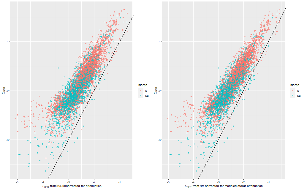
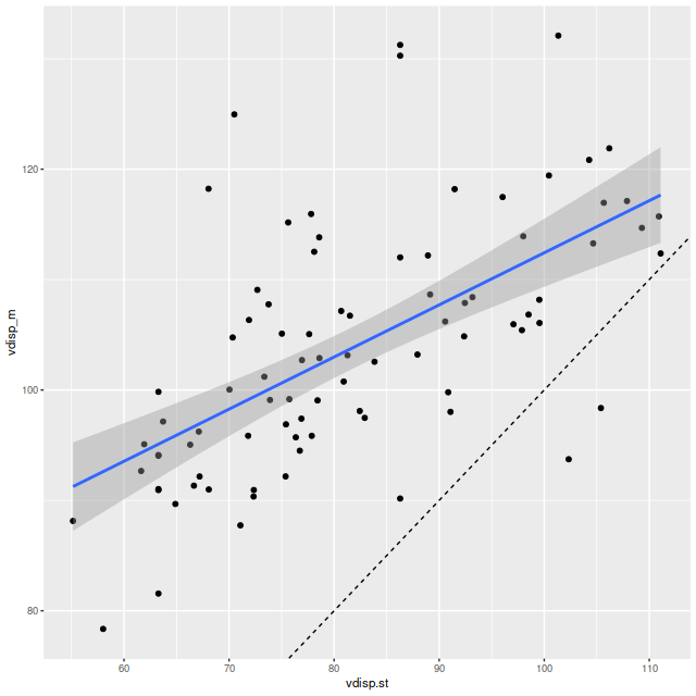
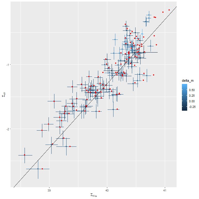
To take a more refined look at this I limited the sample to regions with star forming emission line ratios using the standard BPT diagnostic based on [O III]/Hβ vs. [N II]/Hα. I require at least a 3σ detection in each line to make a classification, so besides limiting the analysis to regions that are in fact (I hope) forming stars it allows correcting Hα attenuation for the observed Balmer decrement since Hβ is by construction at least nominally detected. Now we get the results shown in the plot below. Units and symbols are as before. Hα luminosity is corrected using the Balmer decrement assuming an intrinsic ratio of 2.86 and the same attenuation curve shape as returned by the model. The SFR-Hα calibration line is the thick red one. The blue lines with grey ribbons are from “robust” simple regressions using the function lmrob in the R package robustbase1Correcting for attenuation produced a few significant outliers that bias an ordinary least squares fit and although it’s not specifically intended for measurements with errors this function seems to do a little better than either ordinary or weighted least squares.
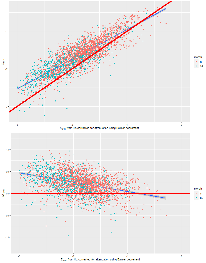
So the model SFR density straddles the calibration line, but with a distinct tilt — regions with relatively low Hα luminosity have higher than expected star formation. To quantify this here is the output from the function lmrob:
Call:
lmrob(formula = sigma_sfr_m ~ sigma_sfr_ha, data = df.sfr)
 \--> method = "MM"
Residuals:
      Min        1Q    Median        3Q       Max
-3.862996 -0.142375  0.004122  0.137030  1.305471

Coefficients:
              Estimate Std. Error t value Pr(>|t|)
(Intercept)  -0.174336   0.019224  -9.069   <2e-16 ***
sigma_sfr_ha  0.785954   0.009948  79.008   <2e-16 ***
---
Signif. codes:  0 ‘***’ 0.001 ‘**’ 0.01 ‘*’ 0.05 ‘.’ 0.1 ‘ ’ 1

Robust residual standard error: 0.2097
Multiple R-squared:  0.7402,	Adjusted R-squared:  0.7401
Convergence in 10 IRWLS iterations

Robustness weights:
 6 observations c(781,802,933,941,2121,2330) are outliers with |weight| = 0 ( < 3.8e-05);
 223 weights are ~= 1. The remaining 2424 ones are summarized as
   Min. 1st Qu.  Median    Mean 3rd Qu.    Max.
 0.0107  0.8692  0.9525  0.9020  0.9854  0.9990
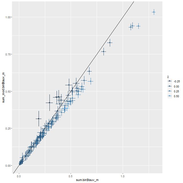
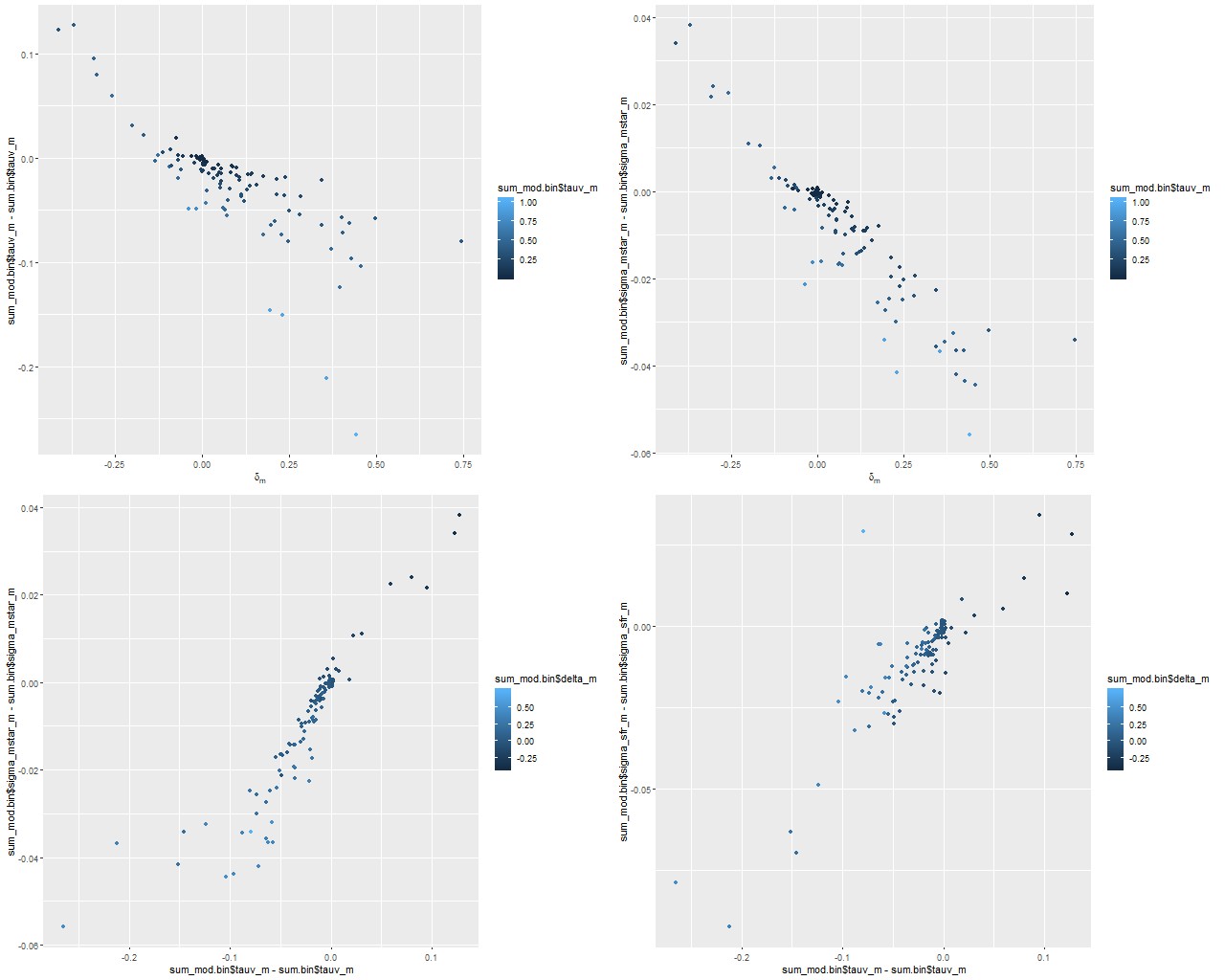
I also ran my Bayesian measurement error model on this data set and got the following estimates for the intercept, slope, and residual standard deviation:
         mean      se_mean          sd       2.5%        25%        50%        75%      97.5%    n_eff      Rhat
b0 -0.1942387 1.943297e-04 0.018346806 -0.2312241 -0.2063781 -0.1943811 -0.1819499 -0.1589849 8913.379 0.9997482
b1  0.7767853 9.828814e-05 0.009436693  0.7579702  0.7706115  0.7768086  0.7830051  0.7949343 9218.014 0.9995628
s   0.2044701 3.837428e-05 0.003319280  0.1981119  0.2021872  0.2043949  0.2067169  0.2110549 7481.821 0.9997152
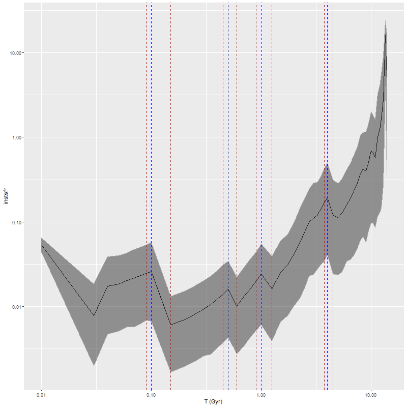
Almost the same! So, how to interpret that slight “tilt”? The obvious comment is that the model results probe a very different time scale — by construction 100 Myr — than Hα (5-10 Myr). As a really toy model consider an isolated, instantaneous burst of star formation. As the population ages its star formation rate will be calculated to be constant from its birth up until 100 Myr when it drops to 0, while its emission line luminosity declines steadily. So its trajectory in the plot above will be horizontally from right to left until it disappears. In fact in spiral galaxies in the local universe star formation is generally localized, usually along the leading edges of arms in grand design spirals. Slightly older populations will be more dispersed.
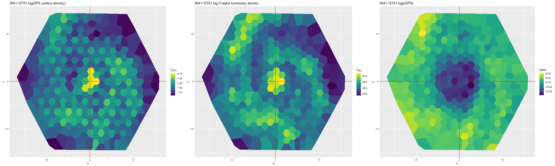
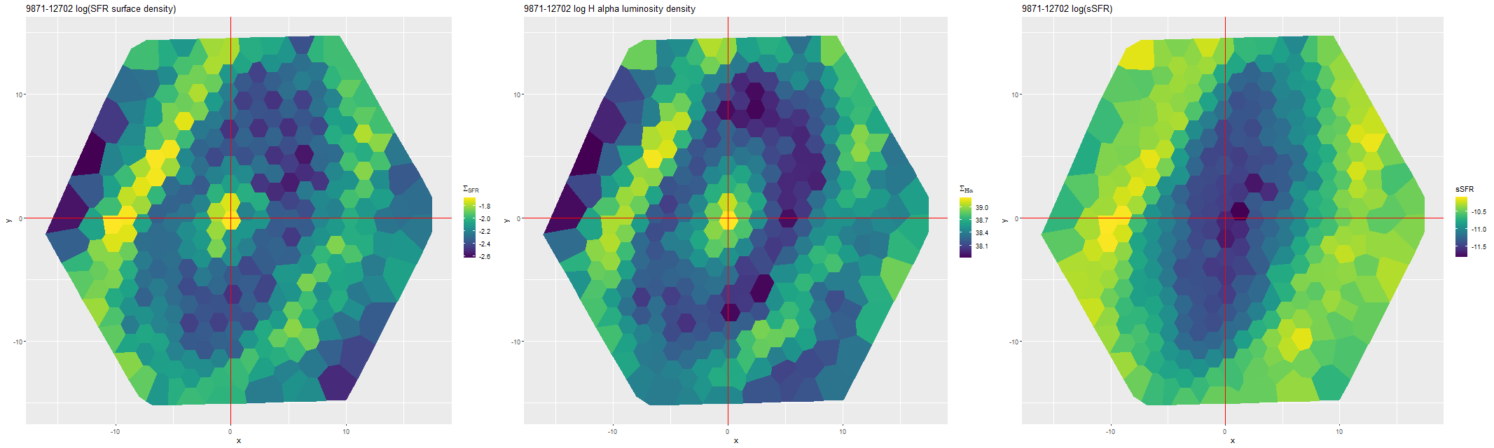
This can be seen pretty clearly in the SFR maps for two galaxies from this sample below. In both cases regions with high star formation rate track the spiral arms closely, but are more diffuse than regions with high Hα luminosity.
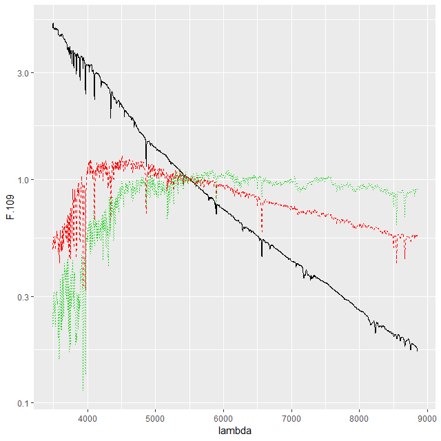
Second topic: the spectral region around the 4000Å “break” has long been known to be sensitive to stellar age. Its use as a quantitative specific star formation rate indicator apparently dates to Brinchmann et al. (2004)2They don’t cite any antecedents and I can’t find any either.. More recently Bluck et al. (2020) used a similar technique at the sub-galactic level on MaNGA galaxies. Both studies use D4000 as a secondary star formation rate indicator, preferring Hα luminosity as the primary SFR calibrator with D4000 reserved for galaxies (or regions) with non-starforming emission line ratios or lacking emission. Oddly, I have been unable to find an actual calibration formula in a slightly better than cursory search of the literature — both of the cited papers present schematic graphs with overlaid curves giving the adopted relationships and approximate uncertainties. The Brinchmann version from the published paper is copied and pasted below.
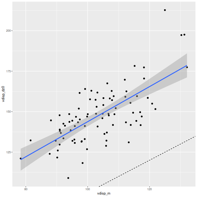
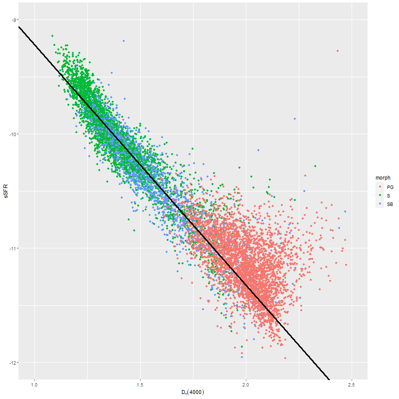
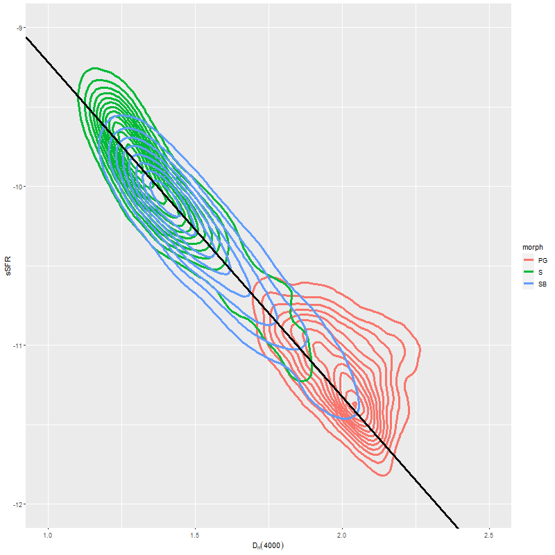
In the two graphs below I’ve added data from the passively evolving Coma cluster sample comprising 3348 binned spectra in 33 galaxies. There are two versions of the same graphs. Individual points are displayed in the first, as before with error bars suppressed to aid (slightly) clarity. The second displays the density of points at arbitrarily spaced contour intervals. The straight line is the “robust” regression line calculated for the spiral sample only, which for the sake of completeness is
\( \log10(sSFR) = -7.11 (\pm 0.02) – 2.11 (\pm 0.015) D_n(4000)\)
Call:
lmrob(formula = ssfr_m ~ d4000_n, data = df.ssfr)
 \--> method = "MM"
Residuals:
       Min         1Q     Median         3Q        Max
-0.9802409 -0.0916555 -0.0005187  0.0962981  7.1748499

Coefficients:
            Estimate Std. Error t value Pr(>|t|)
(Intercept) -7.10757    0.02009  -353.8   <2e-16 ***
d4000_n     -2.10894    0.01418  -148.7   <2e-16 ***
---
Signif. codes:  0 ‘***’ 0.001 ‘**’ 0.01 ‘*’ 0.05 ‘.’ 0.1 ‘ ’ 1

Robust residual standard error: 0.1384
Multiple R-squared:  0.9043,	Adjusted R-squared:  0.9043
Convergence in 13 IRWLS iterations

Robustness weights:
 39 observations c(45,958,1003,1165,1200,1230,1249,1279,1280,1281,1282,1283,1294,1298,1299,1992,2040,2047,2713,2722,2723,2729,2735,2736,2974,3212,3226,3250,3667,3668,3671,3677,3685,3687,3688,3691,4056,4058,4083)
	 are outliers with |weight| <= 1.1e-05 ( < 2.1e-05);
 418 weights are ~= 1. The remaining 4310 ones are summarized as
     Min.   1st Qu.    Median      Mean   3rd Qu.      Max.
0.0001994 0.8684000 0.9514000 0.8911000 0.9850000 0.9990000 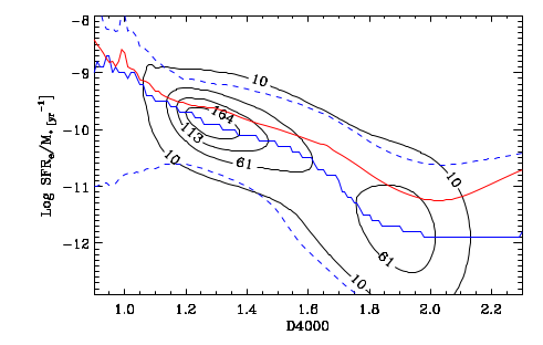
All three groups follow the same relation but with some obvious differences in distribution. The non-barred spiral sample extends to higher star formation rates (either density or sSFR) than barred spirals, which in turn extend into the passively evolving range. The Coma cluster sample has a long tail of high D4000 values (or high specific star formation rates at given D4000) — this is likely because D4000 becomes sensitive to metallicity in older populations and this sample contains some of the most massive (and highest metallicity) galaxies in the local universe. Also, as I’ve noted before these models “want” to produce a smoothly varying mass growth history, which means that even the reddest and deadest elliptical will have some contribution from young populations. This seems to put a floor on modeled specific SFR of ∼10-11.5 yr-1.
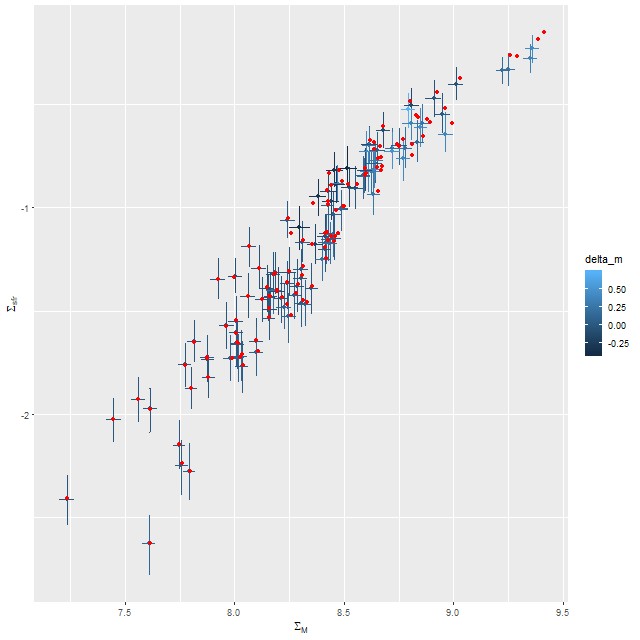
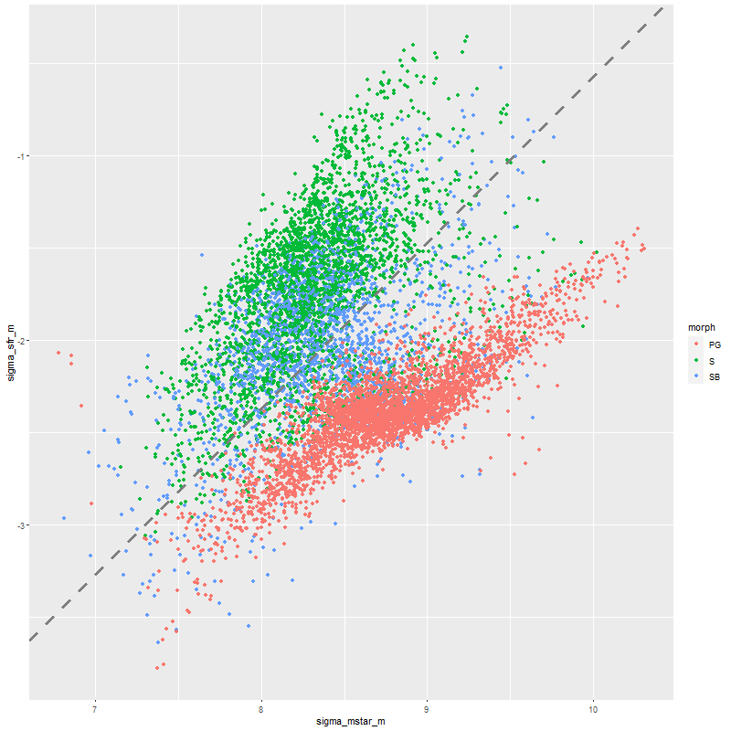
Just to touch briefly on the paper by Fraser-McKelvie et al. barred spirals in this sample do have lower overall star formation than non-barred, with large areas in the green valley or even passively evolving. This sample is too incomplete to say much more. For the sake of having a visualization here is the spatially resolved ΣSFR vs. ΣM* relation. The dashed line is Bluck’s estimate of the star forming “main sequence,” which looks displaced downward compared to my estimates.
Finally, here are a couple of grand design spirals, one barred and one (maybe) not to illustrate how model results track morphological features. In the barred galaxy note that the arms are clearly visible in the SFR maps but they aren’t visible at all in the stellar mass map, which does show the presence of the very prominent bar.


I’m not sure how much more I’m going to do with normal spirals. As I’ve said repeatedly the full sample is much too large for my computing resources.
Next time (probably) I’m going to return to a very small sample of post-starburst galaxies, which I may also return to when the final SDSS public data is released.