I’m returning now to the Leung et al. (2024, 2025) sample of post-starburst galaxies observed in MaNGA. I actually completed model runs for the entire sample some time ago, but it’s taken a while to examine the results and that is still underway. To summarize briefly the sample consists of 48 “central” (CPSB) and 41 “ring” (RPSB)1this classification scheme was proposed by Chen et al. 2019. See also Cheng et al. 2024. galaxies. I analyzed 1255 spectra from the CPSB sample and 2202 from the RPSBs. This was out of 5310 and 7755 spectra in the stacked RSS files that are the sources of my spectroscopic data. I generally tried to bin spectra to a minimum mean SNR of 8 per wavelength bin, although I sometimes accepted less. I excluded spectra that failed to meet whatever threshold I set as well as spectra with foreground star contamination: there were 1311 and 2311 binned spectra in the two subsamples, so I excluded 56 and 109 from analysis.
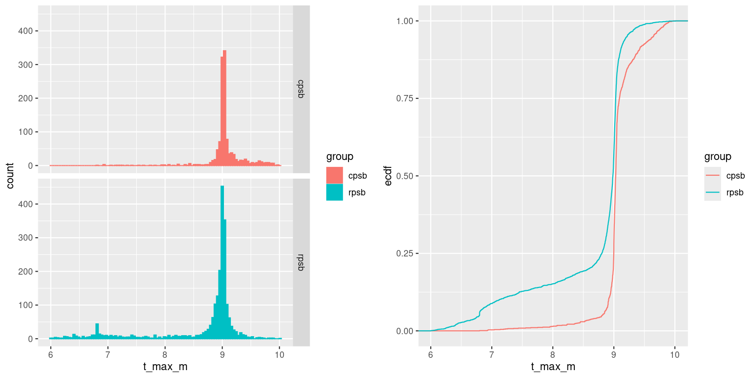
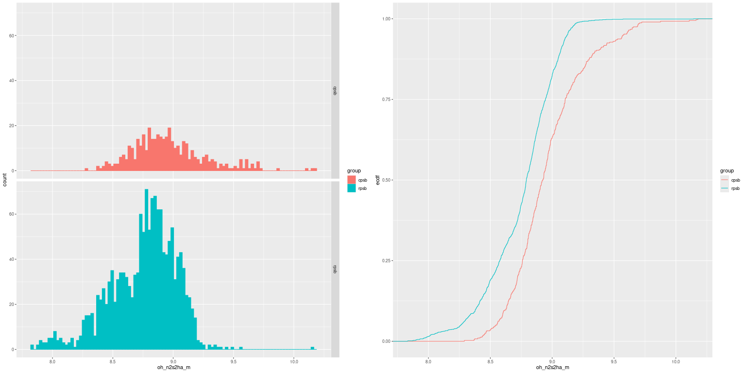
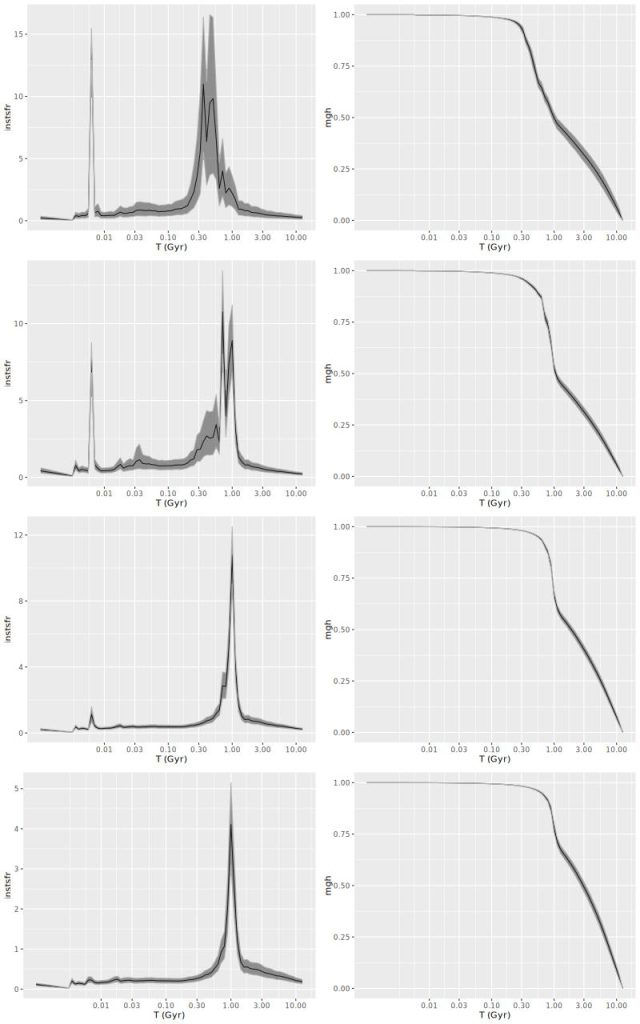
Some time ago while still running models for this sample I mentioned noticing a distinct tendency for model star formation rates to peak at right around 1 Gyr. Since then I’ve added measurements of the lookback time to maximum star formation rate, so I can now check if my visual impression was correct. And, as the graph below shows, it was! This displays on the left histograms of counts of lookback times to maximum SFR, and on the right empirical cumulative distribution functions for the two samples.
Lookback time to epoch of maximum star formation rate by PSB classification
Clearly both have very strong peaks right around 1 Gyr, which again raises the question whether this is a sample selection effect or something in the models or SSP library that’s preferentially producing large contributions from a narrow age range. I’m still investigating this and will follow up in a future post. As a preliminary comment model runs with the BPASS library for a few galaxies show a similar tendency to have very strong peaks but at earlier ages of ~2 Gyr.
The other striking thing here is that the RPSBs have a long tail of more recent peaks: about 5% of the regions are still star forming (peak SFR at < 107 yr) and 15% peaked < 100 Myr ago, while < 2% of CPSB regions peak at < 100 Myr. Standard emission line diagnostics are consistent2these are based on [N II]/Hα vs [O III]/Hβ with Kauffmann’s “composite” region:
No Em
Weak Em
SF
Comp
LI(n)ER
AGN
CPSB
6
62
1
9
16
6
RPSB
2
30
25
26
12
5
Percent of analyzed spectra in BPT diagnostic regions
Regions with LINER and even AGN like emission line ratios aren’t necessarily centrally concentrated, so we can’t infer the presence of AGN from line ratios alone (there are known optical AGN in both samples however).
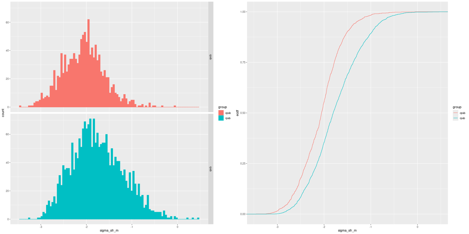
There are other population level differences as well. The RPSBs have higher (in distribution) star formation rate densities:
Distributions of 100 Myr average star formation rate density
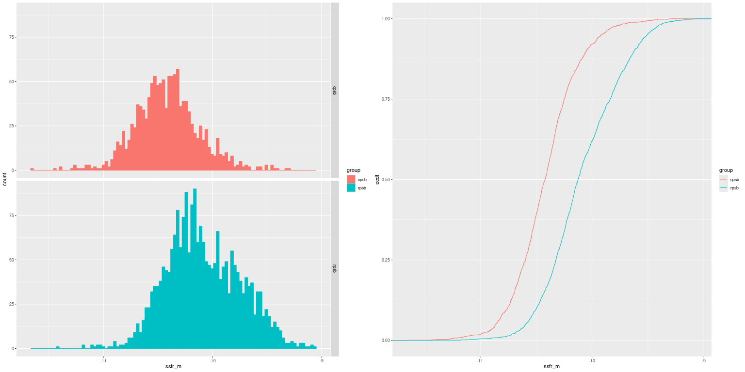
and specific star formation rates (both are 100 Myr averages):
Distributions of 100 Myr average specific star formation rate
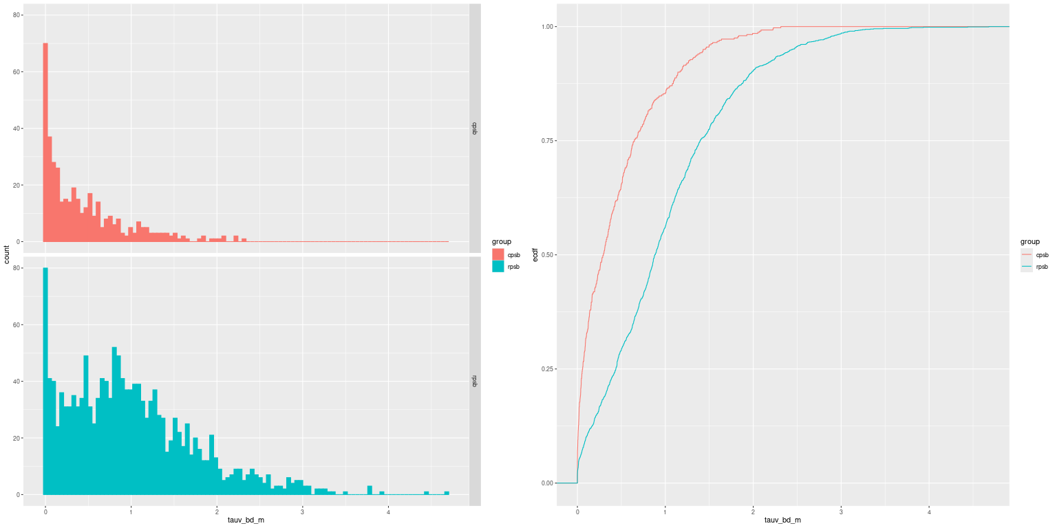
Limiting the samples to regions with firm emission line detections the RPSBs appear to be dustier:
Distributions of τV estimated from Balmer decrement (regions with firm detections only)
and have slightly lower gas phase metallicity:
Gas phase metallicity distributions from [N II], [S II], Hα diagnostic (regions with detections only)
For what it’s worth a Kolmogorov-Smirnov test says all of these empirical CDFs are different at essentially arbitrary significance levels.
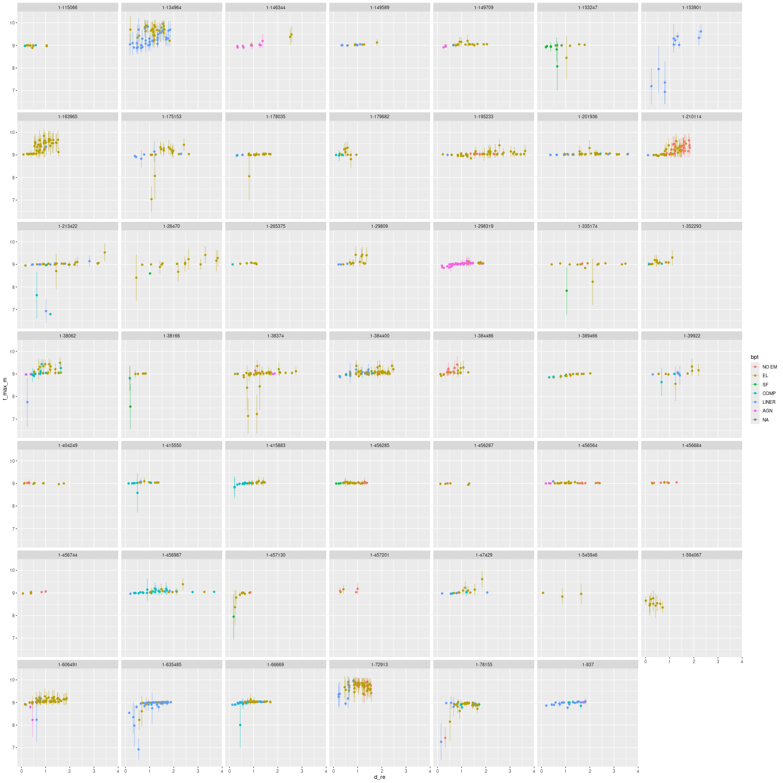
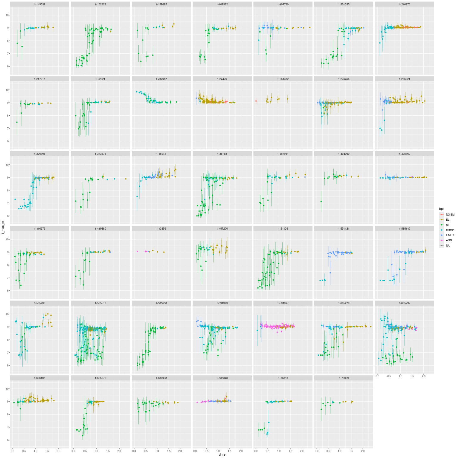
Turning to spatial variations of a few modeled quantities with projected radius for each galaxy and broken down by sample. First is lookback time to maximum SFR:
Lookback time to maximum SFR vs projected distance – CPSB sampleLookback time to maximum SFR vs projected distance – RPSB sample
The CPSBs generally have relatively constant burst ages with projected radius, with a small number having positive gradients — one of the better examples being mangaid 1-635485 (plateifu 7965-1902; row 7, column 2 in the plot above) that I discussed in the previous post. None have negative gradients (center significantly older than farther out).
The RPSBs on the other hand have many examples with positive age gradients. There are also a number of examples of star forming regions interspersed with post-starburst. There’s just one clear example (mangaid 1-232087, plateifu 8152-3703) with a strongly negative age gradient. My models have an old and quiescently evolving central region with a post-starburst disk.
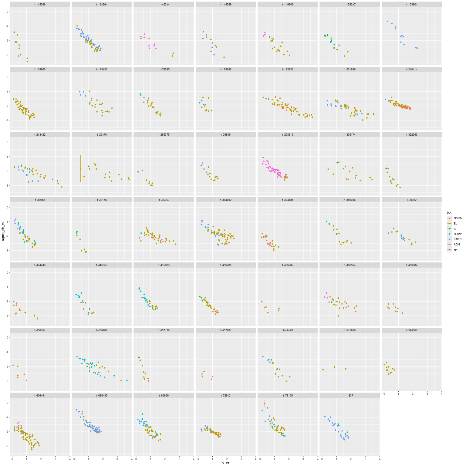
Star formation rate density:
100 Myr average SFR density vs projected radius – CPSB sample100 Myr average SFR density vs projected radius – RPSB sample
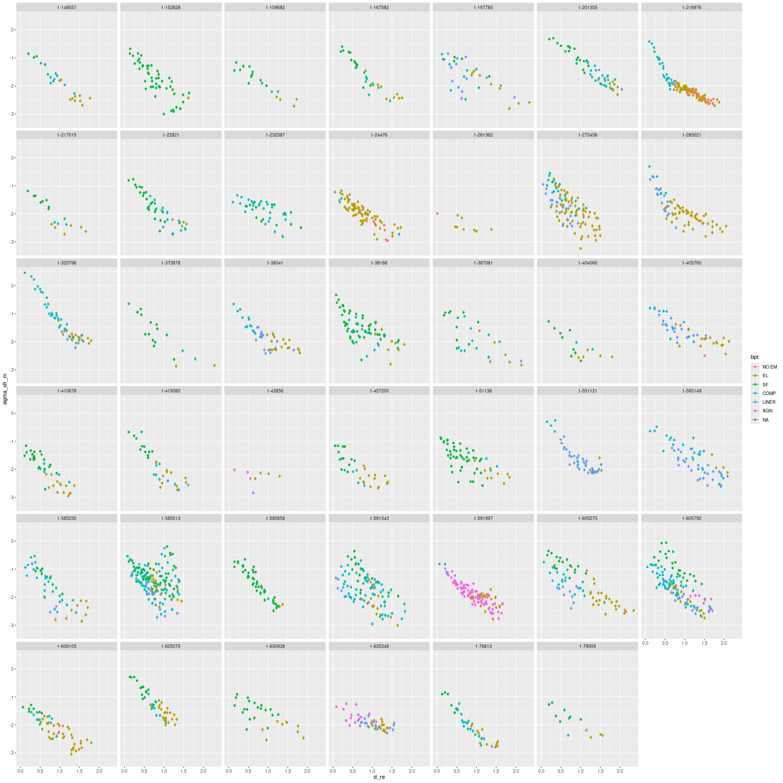
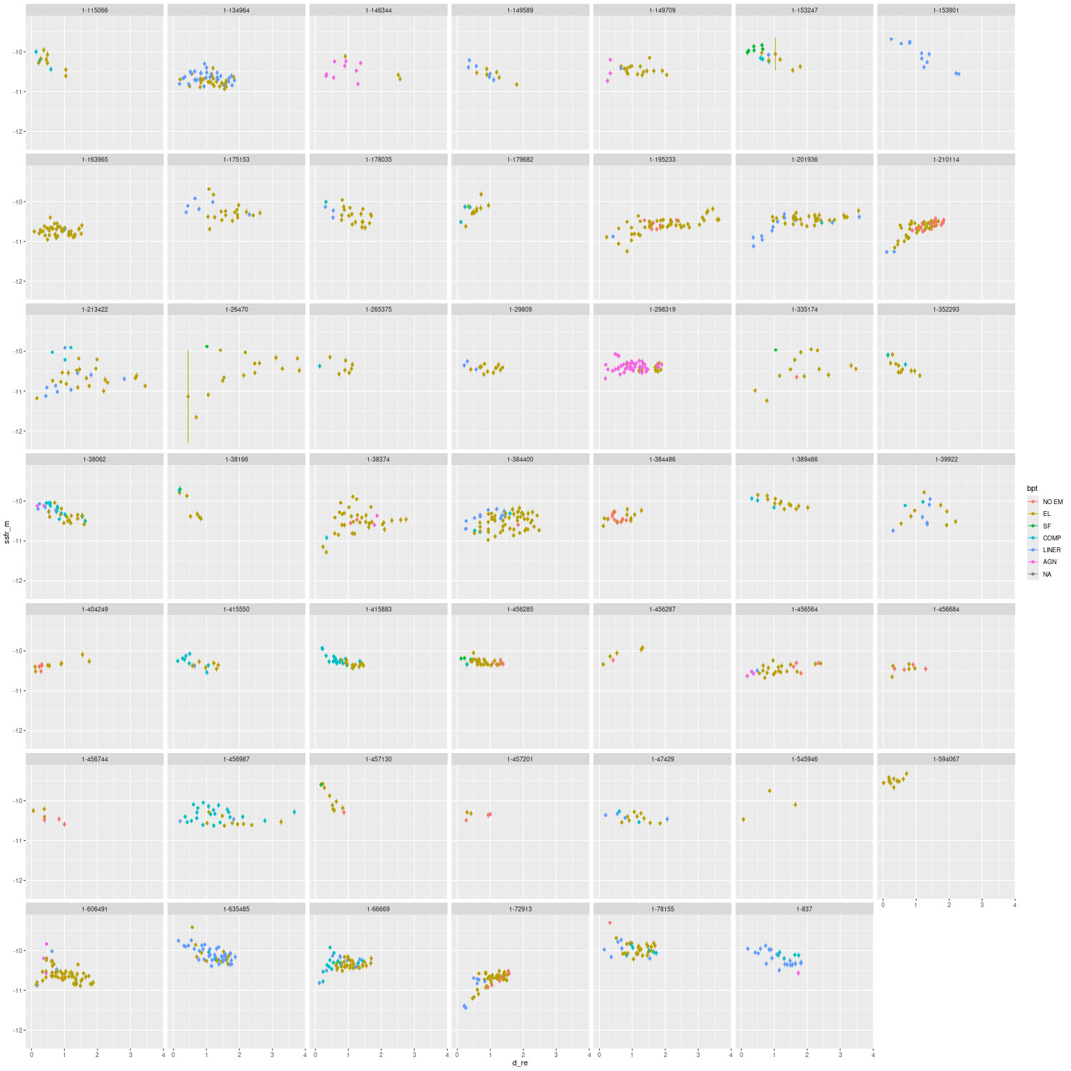
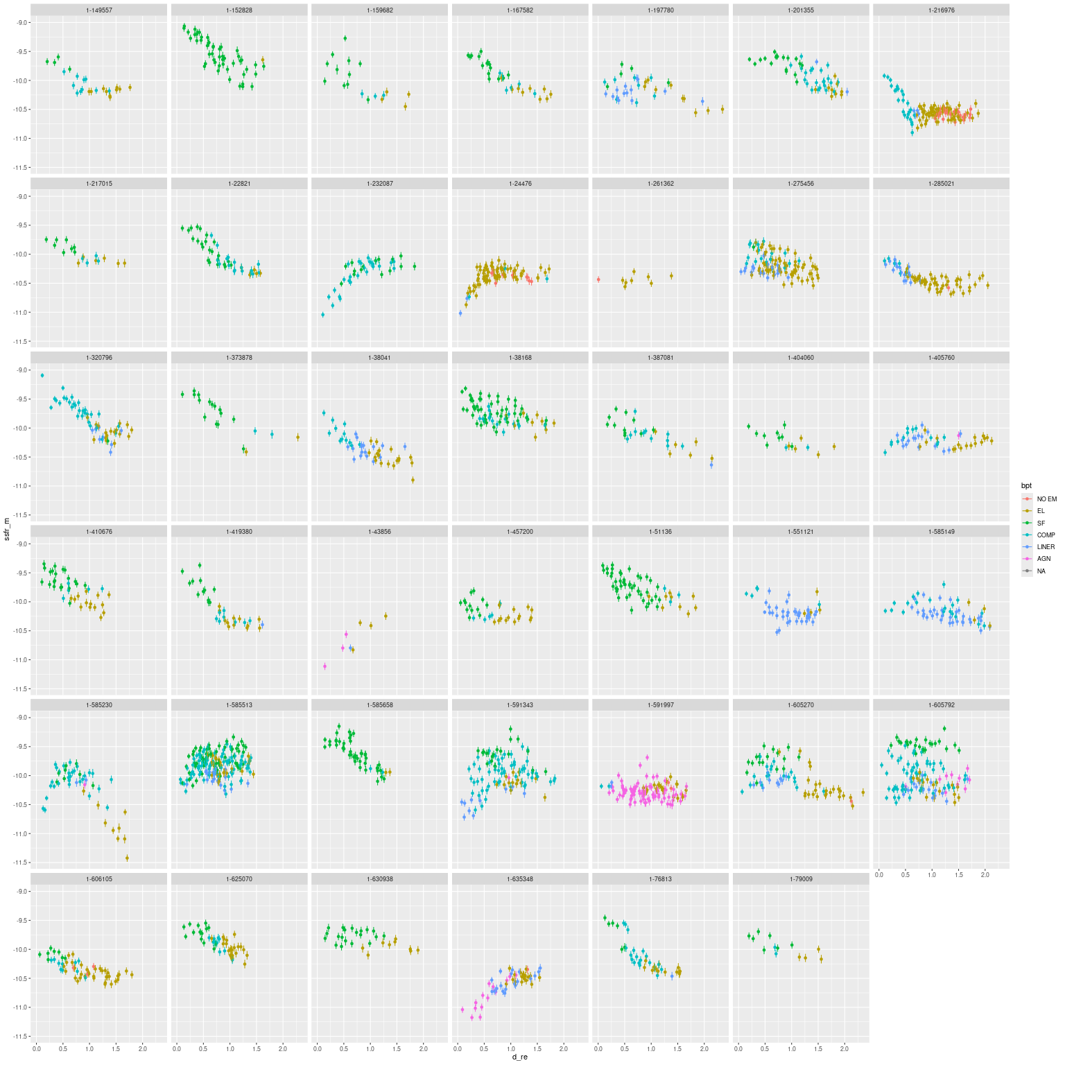
sSFR:
100 Myr average sSFR vs projected radius – CPSB sample100 Myr average sSFR vs projected radius – RPSB sample
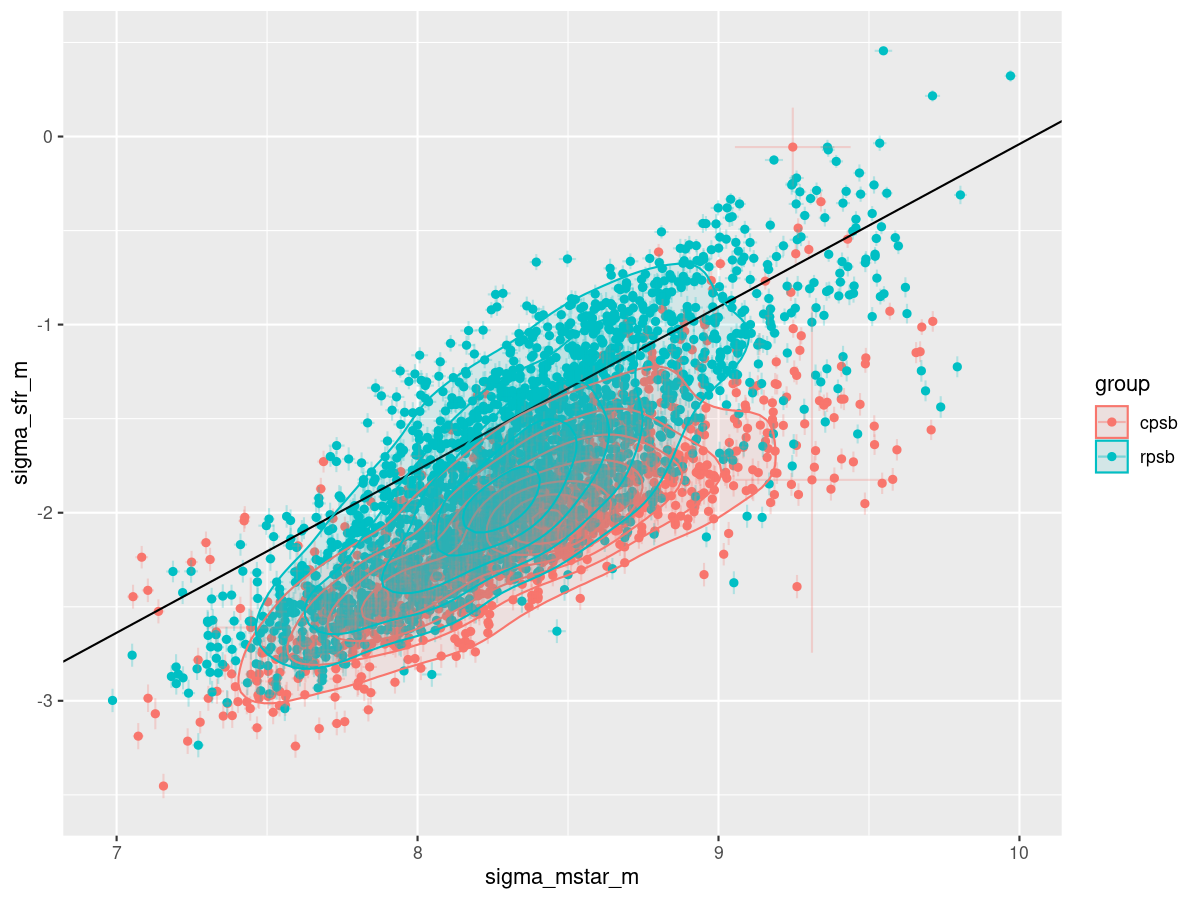
One final plot: (100 Myr averaged) SFR density vs stellar mass density. The solid line is my old calibration of the mean star forming main sequence (which I should recalibrate). Evidently the RPSBs have a larger fraction of regions in the star forming main sequence and conversely the CPSBs extend farther into the green valley.
ΣSFR vs ΣM* – CPSB and RPSB samples
Another thing I found rather odd about the Leung papers is they use some variation of the word “merger” 61 times in two papers, but there’s no indication that they actually examined imaging of their sample, all members of which are in both the SDSS and Legacy Survey footprints. I have examined the entire sample in Legacy Survey imaging3DR9 of Legacy Survey is considerably deeper than SDSS imaging using its custom catalog upload feature with the object list taken from the papers’ supplementary material. What I was mostly looking for was morphology, specifically morphological disturbance. What I found was an interesting difference between the two samples:
Merger
Merger remnant
Disturbed
Total
CPSB
1
7
2
48
RPSB
8
5
6
41
My count of systems with morphological disturbance. Based on visual examination of Legacy Survey imaging.
Almost half of the RPSBs have some level of disturbance, and there are 8 ongoing mergers (or perhaps flybys in a few cases). The mergers are in all stages of Toomre’s famous sequence ranging from M51/M52 like interacting pairs to fully merged systems with prominent tidal tails. There are also several merger remnants that are fully consolidated but with residual tidal tails, shells, and heavily disturbed overall appearance. This suggests either that mergers play a more important role in forming RPSBs, or alternately that we are simply seeing earlier stages of the transition to quiescence in them. I favor the latter: star formation has almost completely shut down in the CPSB sample, while it’s relatively widespread in the RPSBs.
I may return to take a closer look at “interesting” systems, especially the mergers. After that I may look at extending the models somewhat, in particular to include kinematics in the Bayesian part of the analysis.
One thing I found odd about the 2 papers on PSB galaxies by Leung et al. that I’ve used to draw a (probably) final sample is they did no spatially resolved analyses at all, despite the fact their spectroscopic data came from MaNGA. Instead they simply summed all spectra meeting their PSB criteria, calculating a single model star formation history for each galaxy. Recently a paper by the same group showed up on arxiv (2602.13114) that begins to address the issue of spatial variations using what they refer to as a bayesian hierarchical model applied in multiple stages to Voronoi binned spectral cubes. Their approach differs in significant ways from mine: in particular they assign functional forms to the mean behavior of all parameters of their model, so for example the stellar mass density is assumed (on average) to follow a Sersic law. If I understand what they’re doing this will hugely increase the amount of data to be processed in a single model run compared to analyzing each binned spectrum separately. It likely also complicates the geometry of the model and more than proportionately increases execution time. Although they mention no timings the fact that only 3 galaxies were studied in this preliminary paper seems a clue that considerable computational resources were required. Another problem with their approach is it can’t generalize. In particular a small but nontrivial fraction of their sample are clear mergers or varyingly disturbed merger remnants. As we saw in the previous three posts these can have quite complex spatial variations in physical properties.
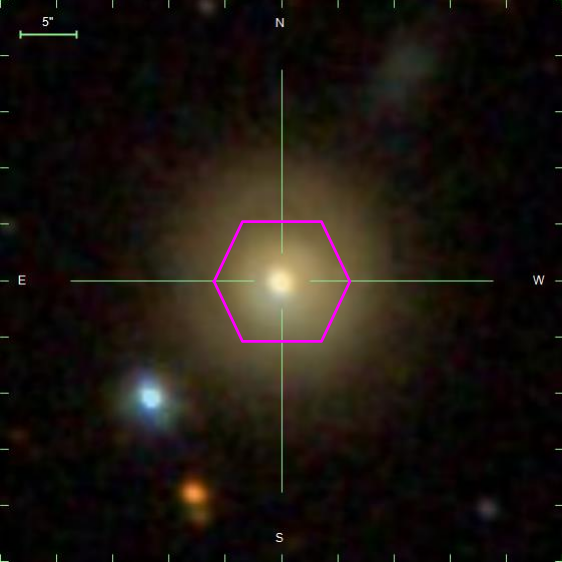
Their models do track some quantities that I also calculate, so it’s worth doing at least a semi-quantitative comparison. I picked just one of their sample for analysis: MaNGA plateifu 7965-1902 (mangaid 1-635485), aka CGCG 375-016. This is an S0 galaxy and a known post-starburst (eg Pracy et al. 2013, who also performed IFU observations). The main reason for the selection was that I was traveling at the time with only a laptop and this set of observations used the smallest 19 fiber science IFU. After binning the RSS file I obtained 52 spectra with SNR > 8. Despite the fact my laptop is mid-range and was bought on clearance at that it worked surprisingly well on this dataset, requiring only about 4 1/2 hours of total sampling time. This was probably at least partly due to the fact that its CPU has 14 cores so I was able to run with 3 threads per chain with a bit of headroom for other tasks.
MaNGA plateifu 7965-1902 (CGCG 375-016) with IFU footprint overlaid. Image from SDSS.
I’m only going to look at a few quantities derived from the models that can be compared to Leung et al. results.
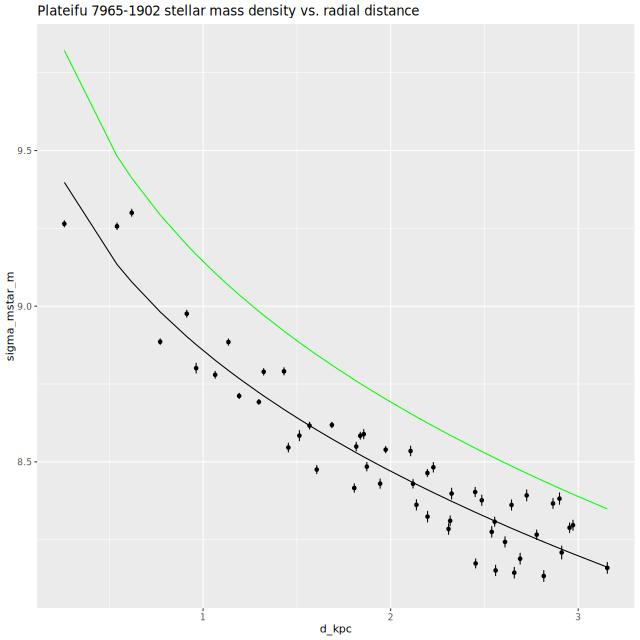
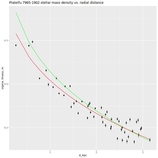
Estimates of present day stellar mass densities are a standard part of my post-processing workflow1the model parameters are simply the contributions of each SSP input model scaled to be approximately fractional light contributions at, roughly, V to the unattenuated light. All derived quantities are generated in post-processing and aren’t part of the model as such. I do most of that in R, although some is done in the “generated quantities” block of the Stan program. . The left hand plot below shows mean estimates of the stellar mass density against projected distance in kiloparsecs from the center. Leung et al. assumed a Sersic relation for the mean, which is shown as the green curve in the plot. I just did an ordinary nonlinear least squares fit to the posterior means, shown as the black line. At first sight the ≈0.2 dex systematic offset seemed a bit concerning, especially since we used the same cosmological parameters and the same stellar IMF (different libraries though). But, a recheck of the manuscript shows (section 4.3.1) that they were estimating the total stellar mass formed, which doesn’t account for mass loss over the lifetime of a SSP. That’s an easy enough calculation to perform, and the revised relation is shown on the right below. Their mean relation has a slightly steeper profile, which is likely due to differences in stellar attenuation estimates — they estimate a higher central attenuation value than I do and use a “greyer” attenuation curve, which requires a higher stellar mass density to produce the observed amount of light.
Perhaps the most significant parameters in their model are the burst age and burst strength. Neither of these are parameters of my model and there isn’t really an unambiguous way to estimate them. What I typically see in post-starbursts is a ramp up to a maximum SFR, a possible plateau with, perhaps, multiple peaks, followed by a more or less rapid decay. The beginning of the ramp up doesn’t necessarily mark the beginning of the burst — in fact it’s most likely an upper limit. Recall from my suite of simulations that the model burst typically began earlier and ramped up more gradually than the input.
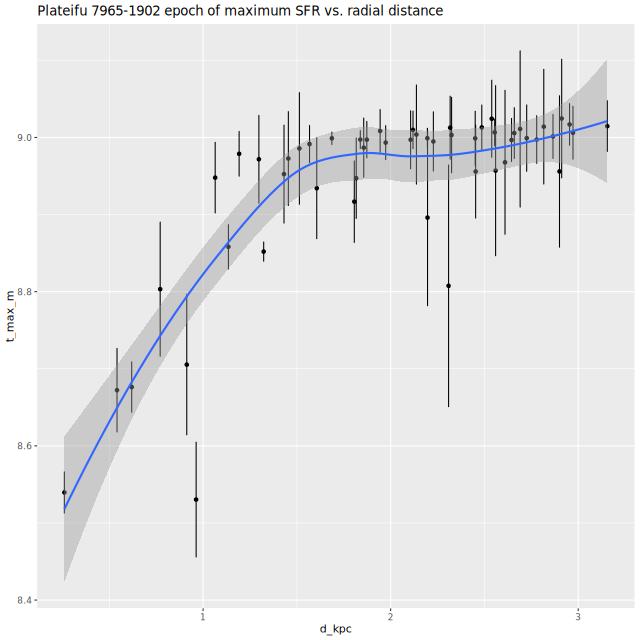
What I can measure unambiguously is the lookback time to the epoch of maximum star formation rate (per the model of course, which may well be biased), so I’ve added that to my post-processing workflow. Below I plot the lookback time to maximum SFR against projected distance. This calculation excludes the most recent 100Myr for a reason I’ll discuss below. The error bars are just ±1 standard deviation in the marginal posteriors. The smooth curve is a loess fit with notional confidence limits, which as always I caution should absolutely not be taken seriously.
MaNGA plateifu 7965-1902 (mangaid 1-635485). Lookback time to epoch of maximum star formation rate.
This plot should be compared to the upper right pane of Leung’s Figure 5. The agreement is rather good overall. I get a range of lookback times of ~1/3 – 1 Gyr, which is close to theirs, but with a steeper gradient in the center. In an earlier IFU based study Pracy et al. found a strong Balmer absorption index gradient in the inner ~1.5 kpc, consistent with my results.
I’ll conclude with plots of model star formation histories, binned over circular annuli. These are shown as both star formation rate and present day mass growth histories. One striking feature of these plots is there appears to have been a recent revival of star formation within about 1reff of the nucleus. Whether this is real is hard to say, but note that the functional form adopted by Leung et al. cannot capture multiple bursts. This galaxy do. es have some ionized gas emission throughout, mostly with “Liner” like line ratios. This could be due in part to some ongoing star formation. In a few bins the very recent SFR exceeds the maximum in the earlier starburst, hence the decision to exclude the recent past in the maximum SFR calculation.
I’m still not sure how to estimate a burst mass fraction. An actual measurement would require a counterfactual estimate of the star formation history in the absence of whatever caused the burst, which we can’t really know. Perhaps a simple interpolation between the pre and post-burst star formation rates would be a reasonable guess if some objective definition of pre and post burst times could be devised. One thing I’ve noticed is mass growth histories of PSB regions usually go from mildly concave to convex for a period of time with a noticeable inflection point where the acceleration in star formation is a maximum. The total mass formed after that inflection point might be a useful proxy (but certainly an overestimate) for the burst fraction. In this case notice that inflection point shifts from ~1Gyr in the inner region to a little older farther out, while the total mass formed since then decreases from ~50% to ~30%. This suggests a negative gradient in burst strength, which is the opposite trend to that estimated by Leung et al.
MaNGA plateifu 7965-1902 (mangaid 1-635485). Star formation and mass growth histories in circular annuli. Outer radii are (0.5, 1, 1.5, 2)reff
One final comment about Leung et al.’s approach. As already noted they assume a functional form for the star formation rate, and specifically they assume an exponential decay model for the preburst evolution starting at some formation time. Although they never discuss this it’s clear from their graphs that the estimated formation times are strongly biased to the young side (see e.g. their Figure 8). For this galaxy for instance the estimated formation times range from just over 4Gyr ago to a little under 6Gyr. This corresponds to a redshift of formation of z≈0.5, which is well past “cosmic noon.” To the best of my knowledge there’s a general consensus that virtually(?) all present day galaxies began forming stars shortly after the Big Bang. While we can’t really say much about the truly ancient star formation histories of galaxies with recent star formation we can say with reasonable confidence that some took place. My non-parametric models always contain non-zero contributions at all ages, with at least plausible mass contributions from very old populations.
I will probably now turn to a more “birds’ eye” view of the entire Leung PSB sample. Since it’s been some time since I did the initial modeling I need to examine the model runs again. There were some with very poor data that need to be culled — these may or may not be the ones Leung excluded from analysis.
By my count there are ~6 obvious mergers in the RPSB sample and ~20 that are to varying degrees disturbed. These are in addition to NGC 2623, which recall was rejected as a candidate CPSB. I may take a separate look at the mergers.
This will be short. I’ve provisionally decided to proceed with the Progeny based SSP model libraries I’ve discussed over the last several posts. I’ve picked two versions for model runs: a “small” one with 5 metallicity bins and 42 age bins from log(T) = 6 to 10.1 in 0.1 dex intervals, and a “medium” sized one with just 3 metallicities (log(Z/Z☉) = {-0.25, 0, +0.5}) and 74 age bins with log(T) = 6.0, 6.5 and 6.55, … , 10.1 in 0.05 dex intervals. These all use the MIST isochrones, Kroupa IMF, and the recommended stellar ingredients from the first Progeny paper. As discussed in a previous post the wavelength interval is limited to 3300 – 9000Å because of the prevalence of terrestrial night sky lines and calibration issues in the near IR portion of MaNGA spectra.
I’ve decided to take one more, maybe final, look at a sample of SDSS selected galaxies in MaNGA. I remembered recently that I’ve made several attempts to select post-starburst samples with various queries of SDSS databases. One I did some time ago had nearly 5800 hits in DR8, with 104 cross matches in MaNGA. Part of the query is pasted below:
select into mydb.mylargerka
  s.ra,
  s.dec,
  s.plate,
  s.mjd,
  s.fiberid,
  s.z,
  s.zErr,
  from specObj s
  left outer join galSpecline as g on s.specObjid = g.specObjid
  left outer join galSpecIndx as gi on s.specObjid = gi.specObjid
  left outer join galSpecExtra as ge on s.specObjid = ge.specObjid
where
  (g.oii_3729_eqw > -5 and g.oii_3729_eqw_err > 0) and
  (gi.lick_hd_a_sub > 4 and gi.lick_hd_a_sub_err > 0) and
  s.z >= .02 and
  (s.snMedian > 10) and
  (s.zWarning = 0 or s.zWarning = 16)
  order by
  s.plate, s.mjd, s.fiberid
So basically this is just a standard sort of post-starburst selection with relaxed limits on both Balmer absorption and emission line strength. The line index data were from the MPA/JHU pipeline, which was last run on DR8.
I had run models for about 1/4 of the 104 galaxy sample when a heat wave arrived, and I decided for the sake of our electric bills not to continue intensive computing 24/7. Temperatures are currently below normal, so I may be able to resume soon. About all I can say so far is the sample contains a mix of known PSBs and false positives — which are mostly ordinary star forming galaxies.
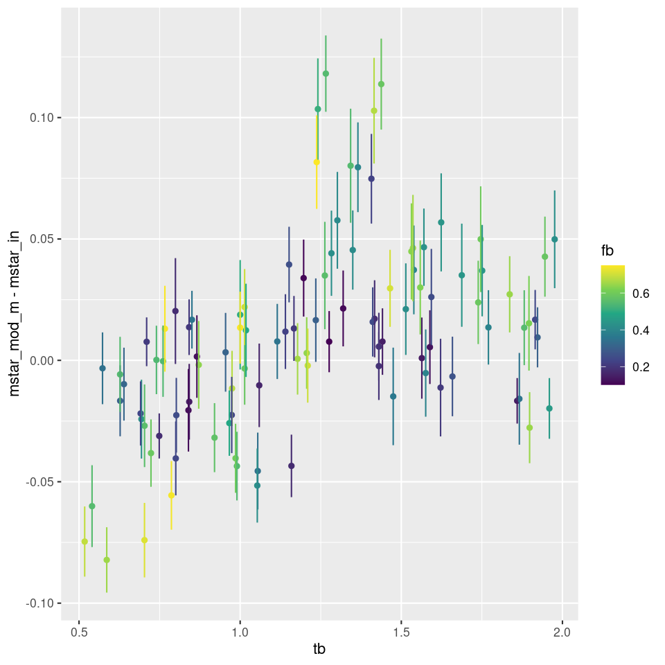
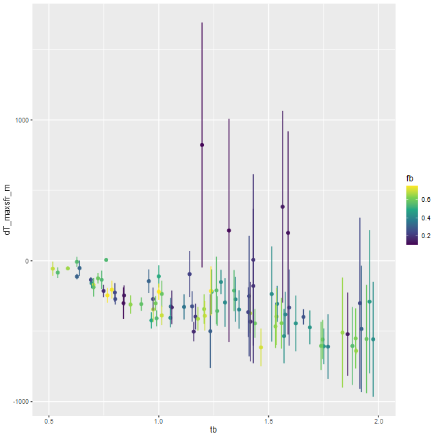
A few brief comments about the simulations, of which I’ve done a few more but will probably bring to an end. First, here is a plot I mentioned but didn’t display last time of the bias in stellar mass estimate against the lookback time to the burst. Points are color coded by burst strength.
Bias is stellar mass estimate vs. lookback time to burst (simulations)
There appears to be a weak trend with burst age up to about 1 Gyr, but at all burst ages and strengths there are biases on both sides of zero. It isn’t clear to me what, if anything else, is driving biases in either direction. The one thing I can say for sure is that the models are overconfident in their ability to estimate the stellar mass since the typical 1σ error bar is under 0.02 dex while the scatter is around ±0.1 dex. I actually think 25% uncertainty in stellar mass estimates is optimistic.
I remembered a short while ago that “outshining” is the term of art in the industry for the situation in which light from recent star formation overwhelms that of the older population. This seems to be a fairly major concern in the literature. A full text search of ADS found 722 instances of its use in the astronomical literature with an explosion of usage after 2006. A quick scan of titles suggests perhaps half of the papers are about SFH modeling. Of course the word is often used in other contexts.
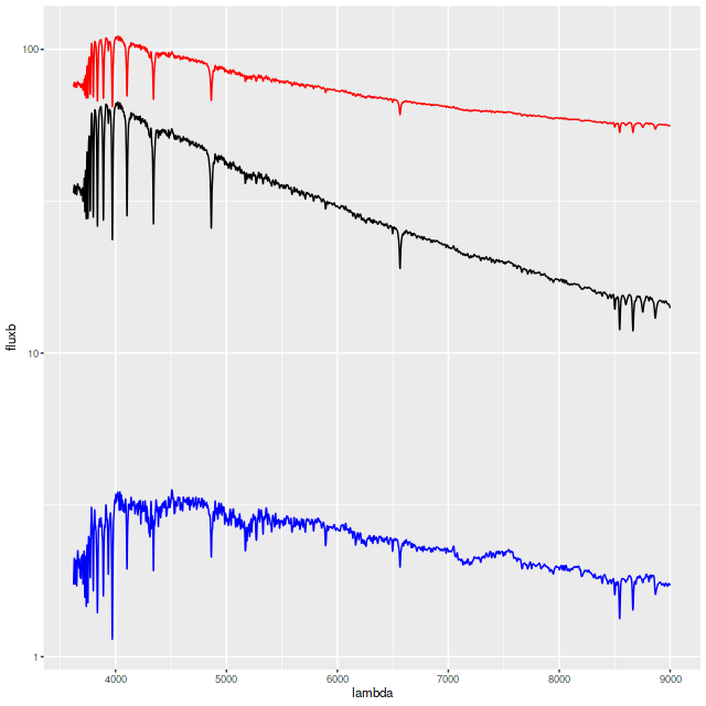
As a slightly more stringent test for outshining I ran one more simulation with a more recent and stronger starburst (tb=0.25 Gyr, fb = 1) than the earlier simulations. Even though the light of the burst population dominates the old base population the latter does have some effect of the combined spectrum (in red below, and offset vertically for clarity): it is redder and the line strengths are altered somewhat relative to the burst population.
Synthetic spectra – strong recent starburst. Fluxes are logarithmically scaled. Total flux (red) is vertically offset.
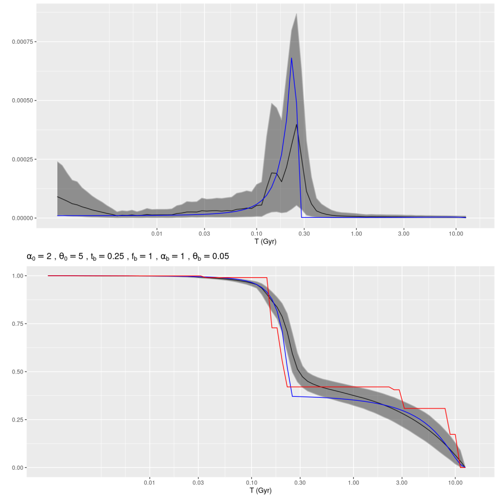
The model actually captures both the ancient and recent star formation history rather well. The mass growth marginal confidence band at old ages covers the input right up to the beginning of the burst build up, and the post-burst SFR is modeled accurately. The total mass in the model slightly exceeds the input: log(M*) = 4.88±0.02 model, 4.84 input. The model specific star formation rate is nearly identical: -9.33±0.08 model, -9.36 input.
Simulation – strong recent starburst
Shortly after starting these simulations I noticed a paper by Suess et al. (2022) describing simulations with a similar objective of testing the ability of a code named PROSPECTOR to recover star formation histories of post-starburst galaxies in the ideal case of inputs matched to the model, i.e. the inputs are used to generate the mock data and then to fit it. I’m not going to say a lot about either the code or paper. IIRC the first published description of the code (Leja et al. 2017) claimed it to be the first to model non-parametric star formation histories in a fully Bayesian framework. As far as I know this is true in the published literature but they only could use a few very broad time bins; the version used in Suess uses 9. I was already using the full time resolution of my adopted SSP model libraries by then.
The 2022 paper only shows a single, no doubt cherry picked example of a fit to mock data. Like mine their model star formation histories fail to cover the inputs for some age ranges. On the other hand their fits to a mock spectrum appear to be rather poor with large systematic errors. In every model run of mine residuals look very much like 0 mean Gaussian white noise with the expected deviance. They appear to show a similar range of deviations from input stellar masses with no significant error in the mean. Another striking similarity is they find a definite floor to late time star formation rates. As I’ve noted many times my models will always include some contribution from very young populations and there seems to be a floor around 10-11.5 /yr in specific star formation rate.
A much more recent paper by the same group (Wang et al. 2025) looked at simulated data from quite different systems, namely ones with bursty star formation on short time scales. Their work was motivated by yet more simulations of galaxy formation in the early universe. I’m again not going to comment much on this paper except to notice that they concluded that “given the correct SFH model, it is indeed possible to infer the SFH by performing SED fitting.” In other words they had to fine tune their prior to get to the right posterior. I’m sure it’s not as tautological as that sentence appears. Anyway, this motivated me to take a brief look at a few multiple burst simulations. The one shown below has two very sharply peaked ones with roughly the same peak SFR but more total mass in the older one. The model has spread out star formation over the entire interval between the input bursts with a slower rise and decay. Once again the maximum likelihood fit obtained with non-negative least squares captures the timing and relative magnitude of the bursts rather well.
Simulation – 2 short starbursts
Recall that my stellar contribution estimates are parametrized as an N-simplex with an implicit Dirichlet prior with concentration parameter α = 1, which is uniform on the simplex. In principle adopting an explicit prior with a concentration parameter < 1 should encourage a more bursty star formation history without favoring any particular ages, and it did (this run used α = 0.25):
Simulation – 2 short starbursts, modified prior
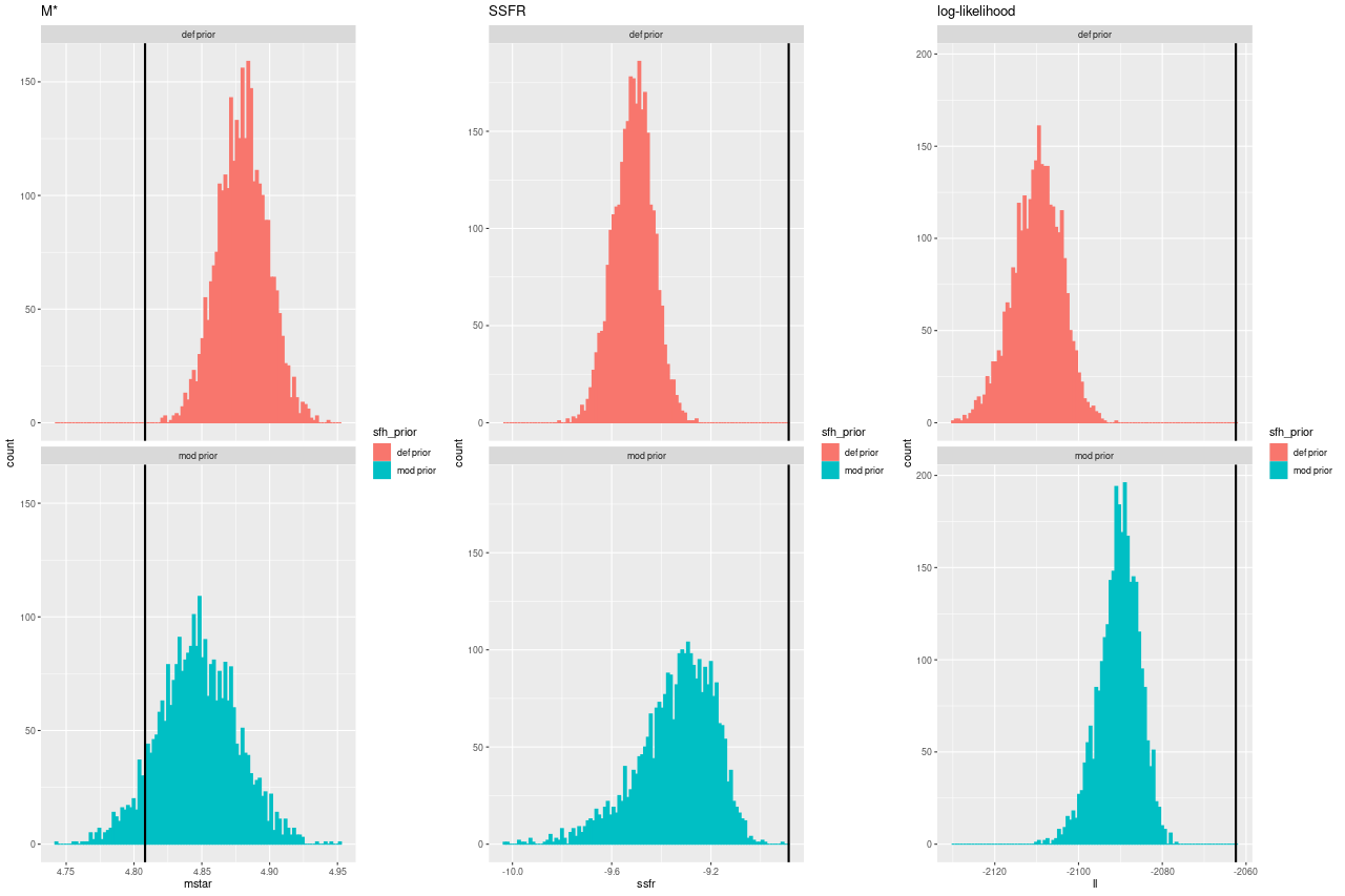
Here are histograms of a few summary quantities I track: the present day stellar mass, specific star formation rate (100 Myr average), and the summed log-likelihood of the fits to the spectra. Both runs underestimated the sSSFR because the recent burst was more spread out in the models.
Two burst simulation: comparing two priors on stellar contributions for sampled stellar mass, SSFR, and log-likelihood of fits
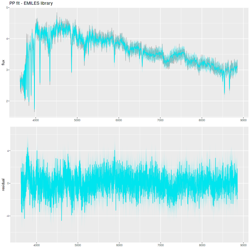
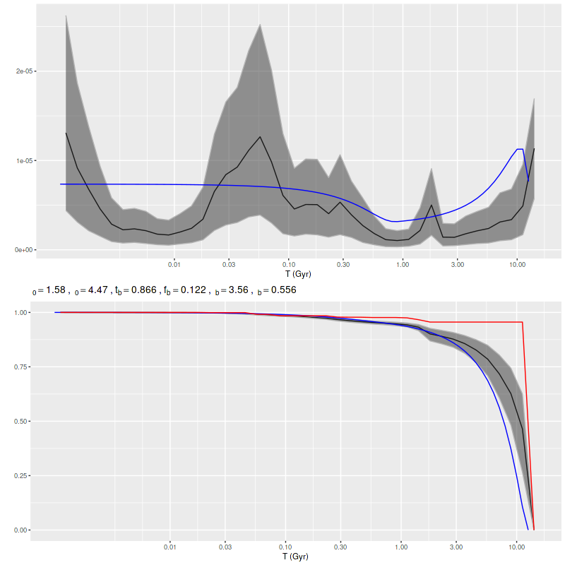
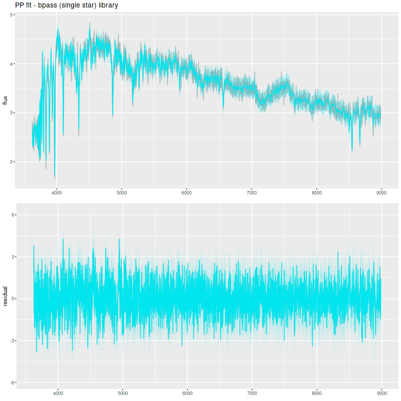
Finally, I did a few runs with two other libraries: EMILES, which has been my base SSP model library for some time, and BPASS with single star evolution and an upper mass limit of 100 M☉. The parameters I used for the star formation history resulted in a gentle late time revival rather than a burst. Both model runs had late time bursts, although the mass added was negligible. The EMILES run has the characteristic jumps at ages where the age intervals change. Although it’s small the BPASS run has the jump at 1.6 Gyr that I noted previously.
Simulation with C3K input and EMILES as test library
As with real data the EMILES models have some systematic errors around the trough around 7000-7300Å, and also in the blue near the Balmer break.
The BPASS models fit the data surprisingly well, despite using completely different sources for stellar atmospheres.
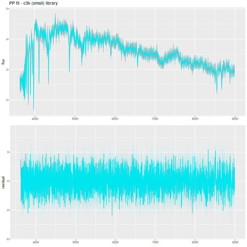
Comparison PP fit with C3K as test library:
The table below summarizes a couple of the quantities I track. The Progeny C3K models that were used to create the inputs recovers them flawlessly. The other two recover the mass (BPASS is low by more than its nominal uncertainty), but are biased on the high side in late time star formation rate estimates.
Stellar mass
sSFR
input
4.78
-9.91
Progeny C3K
4.78 (0.017)
-9.90 (0.054)
EMILES
4.82 (0.012)
-9.62 (0.028)
BPASS
4.67 (0.03)
-9.73 (0.049)
I’m going to get back to real data now using the Progeny generated libraries. The simulations were a useful exercise if for no other reason than to show that timing faded starbursts can’t be done very accurately, at least with full spectrum fitting at visual wavelengths. I did get some ideas for small code improvements, and the idea of stacking star formation rate and mass growth histories seems like a useful visualization tool.
I’ve decided to take a break from real galaxy data and run some simulations of synthetic galaxy spectra. The main motivation was to help make an informed decision about which subset of the ProGeny based SSP libraries to use: the ones based on the MIST isochrones have ages uniformly logarithmically spaced at 0.05 dex intervals and 15 metallicity bins. Most of the latter are considerably sub-solar and aren’t likely to be major contributors to the light of nearby massive galaxies. For possibly metal poor dwarf galaxies it’s always possible to pick a metal poor subset — I have a subset of EMILES that I’ve used for that purpose for some time. More important to me is the choice of age bins. As I mentioned in the last post I did model runs with both 42 (0.1 dex age intervals) and 83 ages, with SSP models younger than log(T) = 6 and older than the currently accepted age of the universe excluded. Since execution time of a Stan model is roughly proportional to the number of parameters and these models are rather time consuming I’d like to know if the coarser age spacing has sufficient resolution. I will show below why it’s correct to exclude the very youngest populations.
Other reasons to do these kinds of exercises are to test the accuracy of retrieval of key quantities in idealized conditions where model assumptions are met by the inputs, to compare different model libraries, or to compare different modeling codes (something I don’t plan to do at present). Performing simulations is de rigueur in the SFH modeling industry and there are many examples in the literature, both as appendices and standalone papers — to name one the second of the two ProGeny papers I linked last time falls in this category. I’ve even done some limited simulations as far back as 2018, but the only case I wrote about was a very simple one.
This time I’ve decided to be more systematic and at least slightly more realistic. Since I remain interested in post-starburst galaxies I am creating simulations with two components: a base population that begins forming stars at the beginning of the universe, which I take to be a lookback time of \(10^{10.125}\) yr. = \(13.36\) Gyr. The second component is a “burst” population that commences star formation at a lookback time of \(\mathsf{t}_b\) with a relative strength of \(\mathsf{f}_b\). The base population has solar metallicity (Z = 0.02) while the burst is slightly subsolar (log(Z/Z☉) = -0.25). This obviously isn’t meant to represent a realistic model for chemical evolution — the purpose again is to test the ability to recover the input stellar metallicities in idealized circumstances. In keeping with my usual attitude of treating this as an afterthought I haven’t gotten around to exploring this issue yet.
Both the base and burst populations have time varying star formation rates proportional to Gamma probability distributions. The Gamma distribution is a two parameter family of univariate functions that can have a fairly wide variety of shapes, all of which have a single mode at \(t \ge 0\) followed by a monotonic decline asymptotically approaching 0. See the table below for the most salient properties. I don’t know of any real astrophysical justification1Abramson et al. (2016) argued for a log-normal form for the evolution of the cosmic SFR density and suggested that this describes the evolution of individual galaxies as well. More recently Katsianis, Yang, and Zheng (2021) argued for a gamma distribution fit to the evolution of the CSFRD and again claimed with some physical motivation that this form holds for individual galaxies. I was unaware of the latter work when I started this exercise. for this choice but it’s notable that it includes two of the most popular parametric forms for modeling star formation histories: exponentially declining (\(\alpha = 1\)), and what’s generally called the “delayed-\(\tau\)” model (\(\alpha =2\)) in the literature. Note that using a probability distribution has nothing to do with probability per se, but a probability density has two useful properties: it’s non-negative on its support and has a finite integral (equal to one when properly normalized).
Given shape and scale parameters the mass in each time bin is proportional to the difference in the cumulative gamma distribution at the beginning and end of each interval. The star formation history for each component is just the mass formed in all age bins, with the burst component multiplied by the burst strength. These are scaled to sum to 1, and the spectra are straightforwardly calculated as matrix products of the input SSP model fluxes with the mass histories. The “flux” values are multiplied by 105 for the sole purpose of making them approximately unit scaled. This has the effect of making the total mass born in the simulated “galaxy” equal to 105 M☉. The fluxes are interpolated to the same logarithmic wavelength grid used by SDSS, convolved with a gaussian to simulate stellar velocity dispersion, then truncated to the wavelength range (3621 Å, 9000 Å). The velocity dispersion is a settable parameter, but so far I have only used 140 km/sec. The base and burst spectra, which were calculated separately for visualization purposes are added, then multiplied by Calzetti attenuation with a user selected optical depth, then finally perturbed with Gaussian random noise. The flux variances are Poisson-like, that is they are proportional to the “counts” in each wavelength bin and scaled to a target average signal to noise. Again this is a settable parameter, but so far I have used a target SNR of 40, which is fairly typical for a fiber spectrum near the center of the IFU of a bright MaNGA galaxy. So far at least I do not add emission lines, but they are allowed in the models.
The subsequent modeling workflow is essentially the same as I use with real data, with some very minor tweaks reflecting the fact that the flux values are arbitrarily scaled. The Stan code is exactly the same as my current working version. Model runs use the same number of warmup and sampling iterations as my real data runs (250 and 750 respectively with 4 independent chains). Post processing is also essentially the same. I extract the posterior predictive fits to the spectra, the model star formation histories, the optical depth of attenuation and the reddening curve slope parameter. I compute the present day stellar mass, the 100 Myr averaged star formation rates, and specific SFR. The stellar mass and SFR are arbitrarily scaled but would scale by the same factor if these were real data from a distant galaxy, so the SSFR would be the same.I also track a few observables: the 4000 Å break index Dn(4000) and HδA.
This time I am exploring a wider range of star formation histories than my previous effort, which only examined a case or two with instantaneous bursts. With seven parameters (plus two more that I’ve held constant so far) it isn’t really practical to do a comprehensive grid of models, so for the most part I have randomly selected parameter values in the ranges shown below. At the time of writing I’ve run a few more than a hundred models. Most of these use the “small” version of the ProGeny C3K base SSP models as the test library, with a few using the input library as the test. I’ve also done a few with the “large” version (see the previous post for details of the ingredients). I plan to do some simulations with the other model libraries I’ve used, especially EMILES, but that’s somewhat of a different project. For now I’m examining the accuracy of outputs for the idealized case where the inputs satisfy the assumptions of the model.
\( \alpha_0 \in [1, 2] \)
\(\theta_0 \in [2, 6] \)
\(\mathsf{t}_b \in [0.5, 2]\)
\(\mathsf{f}_b \in [0.1, 0.75]\)
\( \alpha_b \in [1, 2] \)
\( \theta_b \in [0.01, 0.25] \)
\( \tau_V \in [0.0, 0.5] \)
Here is a cherry-picked example of a fairly strong and recent burst, using the small C3K based library as the test. First is the “observed” spectrum and the replicated values from the posterior (top pane), and the posterior residuals (bottom pane). The residuals look very much like — and pass standard statistical tests for — Gaussian white noise. This is rather different than I usually see with real data, of which a number of examples can be found by scrolling down through previous posts, where there are often large regions of spectra that are systematically misfit. This reflects the fact that all model assumptions are met by the data by construction, so fitting the data is expected.
Simulated spectrum and “posterior predictive” fit and residuals.
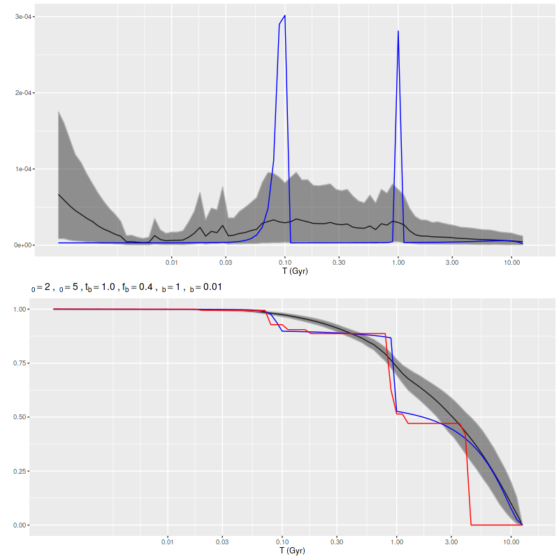
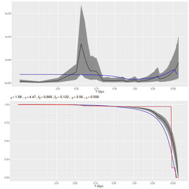
The model star formation history from the same simulated data contains some surprises, and these turn out to be fairly generic features of most model runs. This is a bit of a new graphical display for me. I’ve put the star formation rate history above the mass growth history with the same age scale for each so I can get different views of the same sequence of events. The input model parameters are on a line in between. The blue lines are the input star (mass) formation history. The red line in the second plot is from the preliminary maximum likelihood fit. The black lines and grey ribbons are the marginal means and 95% confidence intervals. Reading from right to left there are several points to note:
The details of the pre-burst SFH are largely lost, although the total mass formed in the model is roughly the same.
The ramp up to the peak of the burst begins sooner and is more gradual than the input. Note that both the input SFR and mass growth are well outside the model confidence intervals in the ramp up period.
Most significantly in my mind at least, the peak of the burst is much later (more recent) in the model than the input. This turned out to be a fairly generic feature of these models.
In this run the post-peak decay is rather steeper on average than the input. In model runs with a rapid input decay the model will usually have a more gradual one.
The input and model SFR eventually converge and the late time model SFH agrees very well with the input, except
There’s an odd upturn in SFR at the very youngest ages (< 3 Myr). This happens to varying degrees in every simulation model run and in all the real data I’ve looked at. It turns out there’s a simple explanation for this. There is virtually no spectroscopic evolution in the relevant wavelength range in the first few Myr of a coeval population’s life. Since the spectra are indistinguishable there is no way to constrain the individual contributions without a more informative prior, and the models are correctly estimating the same marginal distributions for the youngest few populations. Since the time intervals get shorter with decreasing age this produces an apparent upturn in SFR.
Black line and grey ribbon: model results for SFH and MGH. Blue line: input. Red line: MGH from maximum likelihood fit.ProGeny generated SSP model spectra — C3K base models – ages 1-10 Myr, solar metallicityProGeny generated SSP model spectra — C3K base models – ages 1-2 Myr, solar metallicity. Spectra are vertically offset.
There are two surprises in the simulations I’ve run so far. First is that, like the example above, the time of peak star formation in the model burst tends to be biased downwards (more recent) from the input. The bias gets larger in magnitude with increasing lookback time to burst onset and can be as large as several hundred Myr as seen below. The few outliers here were weak bursts with very large variations in the time of maximum SFR.
Bias in time of peak SFR vs. input burst onset time
The other surprise is that the 95% confidence bands of the model star formation histories, whether viewed as SFR or mass growth histories, fail to cover the inputs for at least some epochs around the time of the burst. In other words the models are saying that the actual input star formation histories are highly unlikely. Why is this?
It’s not, I think, because of any convergence failure. Stan is quite aggressive at flagging potential issues and there were virtually none in any of the model runs. I also don’t think it’s because the model runs were too short. I’ve occasionally gathered much larger samples with longer warmup times as well and except for exploring the tails of the distributions a little more thoroughly there is little change in marginal 95% confidence intervals.
Most of the model runs were done with the reduced size SSP library with just half of the available age bins (0.1 dex intervals). This doesn’t seem to have reduced the real effective age resolution, but in the small number of runs I did with the full set of ages the marginal contributions have larger confidence intervals, so this could increase the coverage.
I suspect though that the prior on the star formation history is having a larger effect than I would have suspected. The main clues here are the maximum likelihood fits. which often produce mass growth histories (the red lines in the plot above and the ones below the fold below) that are rather close to the input MGH, also falling outside the 95% model confidence bands for at least some epochs. In my current workflow the slightly perturbed maximum likelihood solution is used to initialize the Stan model. In most of the model runs the samples quickly move away from the initial values. While the fits to the data are good in all model runs the summed log-likelihood of the sample spectra is always less than the maximum likelihood solution, in the sample shown below by about 7%.
Log-likelihood of posterior samples and maximum likelihood solution for a simulated model run
Below the fold I’ve posted some more cherry picked examples of model star formation histories. A few general comments about them:
The late time star formation rate is generally well captured by the models.
The ancient (pre burst) star formation history is sometimes captured well with weak bursts. Particulary noteworthy is the second example below, which has a recent and weak burst with a gradual ramp up and decay. The entire star formation history is modeled accurately. In the literature there are sometimes references to “outshining” or a “dazzle” effect in (post)-starburst galaxies. This seems to be a real thing.
Early time bursts aren’t necessarily recognizable as such. In some cases the model just shows an extended period of star formation followed by more or less gradual quenching. I believe this is consistent with some claims in the literature, but I don’t care to look for the relevant papers right now.
I’ll conclude with a look at results for all simulation runs (so far) for some of the summary quantities I track. First, the present day stellar mass is on average unbiased but in individual runs there are errors as large as ±0.1 dex. The typical posterior uncertainties are only ~0.01 dex, so the models are consistently too optimistic. I’ve noted this in real data, which shows similar nominal uncertainties with moderately high S/N data.
Not shown here but I did notice a weak dependence on the input burst onset time or time of maximum SFR in the sense that recent bursts tend to underestimate the stellar mass. This is another possible manifestation of the “outshining” effect.
Error in model stellar mass vs. input stellar mass
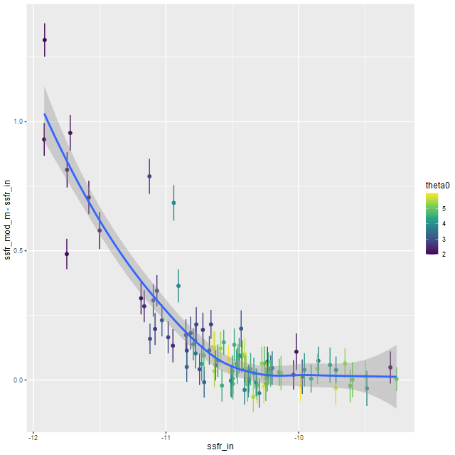
The most dramatic bias is a tendency to overestimate the specific star formation rate when the input SSFR is low. This is also something I’ve seen in real data: as I’ve noted a time or two even the reddest and deadest of ellipticals seem to have a floor of about -11.5 for the estimated SSFR.
One thing I didn’t think about until finishing this analysis is that the contribution estimates tend to be skewed to the right when they’re near 0, so the median might be a better estimate of central tendency than the mean. That might make a (probably) small difference. I will look into this.
Error in model specific star formation rate vs. input SSFR
Finally, there’s a nearly linear relation between the error in the posterior estimate of the optical depth of attenuation and the input. Note also the stratification of the reddening slope parameter δ: at relatively high input optical depths the largest departures have the reddest attenuation curves. I think this behavior is directly related to the prior. Since I don’t think the attenuation is very well constrained by the data I use fairly informative priors on both the optical depth and slope parameter; both priors are truncated normals with a lower bound of 0 for τV and a range of (-0.5,1.2) for δ. This is an easy thing to test simply by changing the priors for these parameters.
Mean and standard deviation of model optical depth – input optical depth vs. input optical depth
I am not quite finished with these simulations. I want to expand the range of input parameters a little bit, and I need to look a little more carefully at subsets of the ProGeny SSP models. The main result so far is that my hopes of timing key events in post-starburst galaxies’ histories were probably too optimistic.
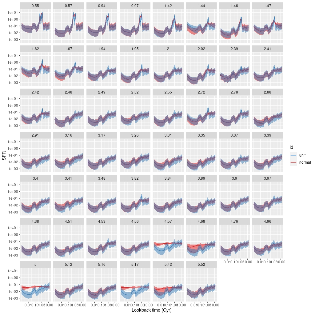
After my not so insightful realization recounted last time that my attempt to modify the prior on star formation histories wasn’t actually doing anything I thought a little further about how to specify one. Gaussians are always popular choices for priors, so why not give them a try? For a first cut I added the following lines to the “transformed data” section of the Stan model:
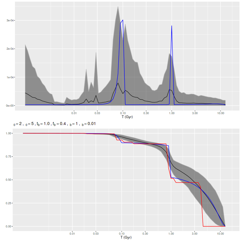
Even though the prior allows values of the stellar contributions that are infeasible given the simplex declaration this causes no technical problems: the models sample without complaint and parameters satisfy all constraints. Execution times are comparable to the original model formulation and convergence diagnostics are OK. But, the model runs had some unexpected features. I did a set of model runs for a single MaNGA galaxy from the post-starburst ancillary sample — mangaid 1-201936 (plateifu 10220-3703). Model star formation histories compared to the original model are shown below for the 58 binned spectra:
MaNGA plateifu 10220-3703 (mangaid 1-201936). Model star formation histories with two different SFH priors.
What’s striking here is that several of the spectra in the low S/N outskirts of the galaxy have nearly constant star formation rates with very little sample variation. In other words the models are basically returning the priors. The cause of this behavior isn’t quite clear. Relatively low signal to noise seems to be necessary, but not sufficient since similarly noisy spectra have essentially the same SFH’s as the original model formulation. It also isn’t due to convergence failure because much longer runs with more adaptation iterations show the same behavior. It is possible perhaps that the posteriors are significantly multimodal and Stan is preferentially falling into one of them. Notable also is that the fits to the data measured by log-likelihood are virtually identical even for the runs with the anomalous SFH’s. At the very least this tells us that uncertainties in quantities derived from the models are considerably larger than within model run variations — of course I have always believed this and said so a number of times.
After trying several variations on this theme that either had none at all or undesirable effects on sampling, and after some additional consideration I think that, given the model parametrization, the uniform on the simplex prior for stellar contributions is actually the one I want. That leaves the question of what, if anything, to do about the abrupt jumps in model star formation rates.
One possibility is simply to redefine the endpoints of the age bins to be, say, halfway between nominal SSP ages instead of at the model ages as is my current practice. In the case of the EMILES library this would mean for example that the 3.75, 4, 4.5 Gyr bins would have widths of 0.25, 0.375, 0.5 Gyr instead of the present 0.25, 0.25, 0.5. This involves no change to the actual model runs at all, so most quantities derived from the models are unchanged.
Another solution is to adopt a library with a more uniform age progression. One with approximately equal increments in log age seems preferred. As yet there have been no published updates to the MaStar based SSP libraries mentioned last time, so I’m waiting for them, while still considering generating my own.
I’m going to briefly return to BPASS based models. After that I’m not sure.
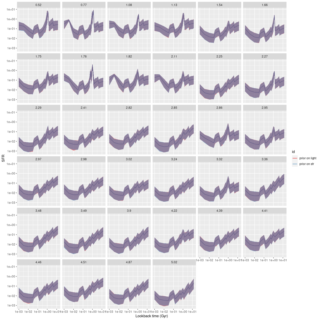
One thing I’ve wondered about for a while is the extent that priors on SSP model contributions affect modeled star formation histories. Previous experience suggests not much at all unless the prior is highly constraining. To be a little more specific in my current workflow I normalize the SSP model spectra to have average flux values of 1 in (approximately) the V band, and also adjust the galaxy fluxes in the same way. In the Stan model the stellar contribution parameters are declared as a simplex, that is a vector with non-zero elements summing to 1. That makes the parameter values the fractional contributions to the (unreddened) galaxy flux at V. My current working code doesn’t provide an explicit prior for the stellar parameters, but they have an implicit proper prior of a uniform distribution on the appropriate dimensional simplex. More technically the prior is a Dirichlet distribution with all concentration parameters equal to 1. Note the marginal distributions aren’t uniform, but they are all the same. One implication of that is that a typical draw from the prior1Stan doesn’t sample from the prior even for initialization, but of course the prior influences the posterior through Bayes’ rule. will have jumps in the star formation rate at exactly the times where the width of the age bins jump, a problem that I’ve noted several times before.
A possible solution to this problem is simply to alter the prior to encourage smoothly varying star formation rate rather than smoothly varying light contributions. It turns out I’ve been feeding my Stan code the data I need to do that: the initial mass in a given model SSP is inversely proportional to the normalization factor applied to the spectrum, and the star formation rate is just the mass divided by the time interval assigned to the SSP. Both of those quantities are passed as data to the Stan model even though they weren’t used in any way previously. I added just 3 lines to the code to change the prior on the stellar contributions. In the “transfored data” section
If I did this right the prior is completely agnostic to any star formation history, whereas the previous implicit prior was completely agnostic to any run of light contributions.
The modified code compiled without complaint and there’s no discernible difference in either execution time or convergence diagnostics.
I’ve only run this on one set of galaxy data, from MaNGA plateifu 8565-3703 (mangaid 1-92735). This is one of Schawinski’s “blue early type galaxies,” chosen mostly because the data were binned to just 34 spectra so a complete set of model runs only took a few hours. And, as seen below the other things that don’t change are the modeled star formation histories.
Plateifu 8565-3703 (mangaid 1-92735). Star formation history models with two distinct priors on stellar contributions.
I need to do some more validation exercises, but it appears my long ago conclusion that the choice of prior on the star formation history has little effect was correct. The data dominates the model outcome through the likelihood.
Update
Since I hit publish a few days ago I realized two things. First, the weights I applied to the stellar contributions to “encourage” a smoothly varying star formation rate were inverted. What I should have used was:
The second thing I realized is this makes no difference at all given the form of the prior. The transformation simply maps a point on the simplex to another point on the simplex that has exactly the same probability density since by construction the prior is uniform on the simplex.
So, it should have been expected, and it’s a good thing that it in fact happened that the model runs produced the same results. What happens if I use the following prior, with the weights supplying the parameters for the Dirichlet?
target += dirichlet_lupdf(b_st_s | norm_sfr);
This failed to sample almost always. I’m not entirely sure why, but I suspect this turns a problem with relatively simple geometry at least with regards to the prior to one with a complex and troublesome geometry.
This little experiment actually told me nothing about the effect of priors on model star formation histories. Two of the priors are actually the same, and the third fails for reasons that aren’t completely clear. I may experiment with different forms of prior. I’m still, of course, looking for a new SSP model library.
When I was doing my initial fits to the M31 MaNGA spectra I noted two that I initially thought were contaminated by foreground stars, and therefore I masked them to prevent further analysis. One of the two, in MaNGA plateifu 9677-12701 (mangaid 52-8) is a certain foreground star and won’t be discussed further. The other, in plateifu 9678-12703 (mangaid 52-23), turns out to be a luminous red supergiant that’s a genuine resident of M31. This is confirmed by two nearly contemporaneous catalogs of M31 red supergiants: the one by Ren et al. (2021) that I noted previously and Massey et al. (2021), which I stumbled upon more recently.
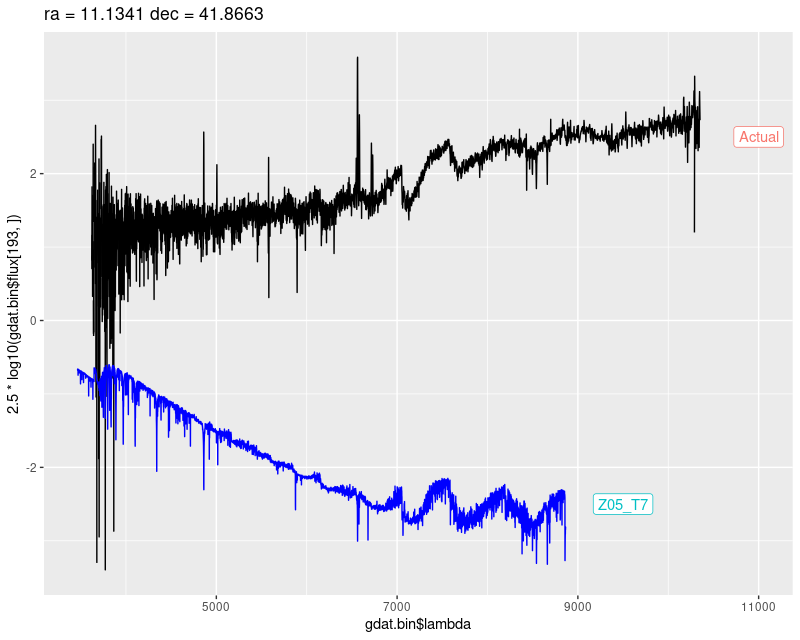
In fact there are two comparably bright red supergiants in this IFU. One that’s about 9″ north of the masked one probably should have been masked by whatever criteria I used, but it’s likely I failed to notice the fit to the data since I don’t have the patience to look at every spectrum and data fit that pops up. So, here is the spectrum, displayed in (negative) magnitudes with arbitrary zero point. The blue spectrum is the closest match in my SSP library, a 10 Myr old population with the highest metallicity I used (2.5 Z☉. This is one of the theoretical spectra from PyPopstar). This sorta looks right except it’s much too blue. The solution to that is, of course, to add some reddening through dust attenuation.
plateifu 9678-12703 (M31 10 kpc ring)
Spectrum contaminated with red supergiant and closest match SSP model spectrum
The maximum likelihood (non-negative weighted least squares) fit did just that, with only a single stellar contributor and a very high dust attenuation of τV = 3.0. This still doesn’t quite work: the residuals are rather strongly sloped in the blue and the details of the absorption features in the red aren’t quite right.
plateifu 9678-12703 – NNLS fit to spectrum contaminated with red supergiant
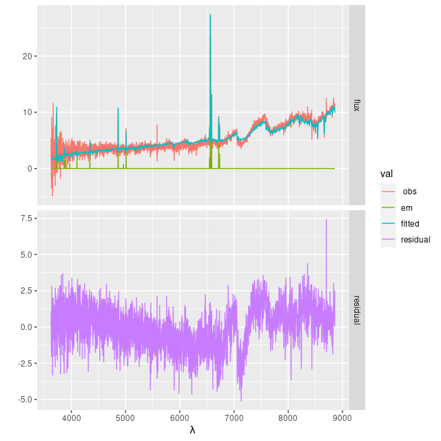
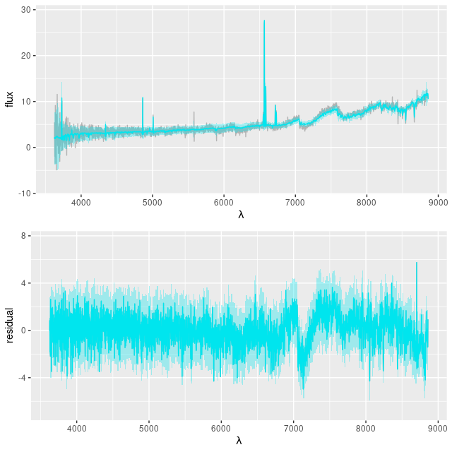
I still use a Calzetti attenuation relation in my NNLS fits. The Bayesian fits using Stan have the more flexible attenuation prescription that I described back in this post, and that helped considerably with the continuum as seen in the plot below. The absorption features in the red still aren’t fit well. The model has an even more extreme attenuation estimate with a much “grayer” than Calzetti slope, with τV = 4.38 ± 0.05 and δ = -0.33 ± 0.011see the link above for the meaning of these parameters.
9678-12703 – posterior predictive fit to spectrum
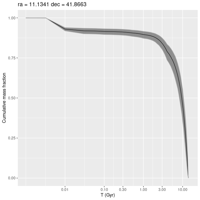
The model star formation history (displayed as a mass growth history below) isn’t completely implausible. The presence of a very luminous evolved star indicates the region is at least some Myr old, and a rapid onset and decline of star formation is typical for star forming regions in mature spirals. The recent episode of star formation added about 7% to the present day stellar mass, while at least 60% was in place by 8 Gyr ago (per the model).
plateifu 9678-12703 (M31 10 kpc ring)
Model mass growth history for a region containing a bright red supergiant
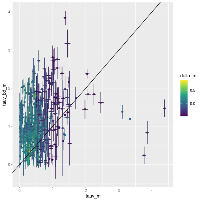
Nevertheless I consider the model results to be highly suspect, mainly based on the very large optical depth. Massey estimates the attenuation for the red supergiant to be AV ≈ 1.18, although this is apparently based on a formula rather than a direct empirical estimate. But another piece of evidence that’s close to a smoking gun is an estimate based on the Balmer decrement of emission. Despite the lack of apparent ionizing sources outside the bright H II regions in the west there is widespread diffuse emission in this region with star-forming like line ratios. The estimated optical depth derived from the Balmer decrement for this region is τV, bd = 1.47 ± 0.23 (1σ), reasonably consistent with the Massey estimate and with the values derived for the rest of the IFU.
How widespread a problem is this? Below I plot the Balmer decrement derived optical depths against the stellar based estimates for all spectra in M31 MaNGA with star forming emission line ratios, about 11% of the entire sample. The 5 most extreme outliers are in this IFU in the regions surrounding the two bright red supergiants (the masked spectrum would also be in this region of the plot). The same 5 regions are also extreme outliers in the SFR vs. stellar mass and SFR vs. Hα plots that I showed early on. So, even though there are many cataloged supergiants in the study region these two appear to be uniquely bright and to have had the largest impact on model results.
M31 MaNGA – Optical depth off attenuation estimated from Balmer decrement vs. model values of τV
Of course there are hotter bright stars in the study area and these could affect results in different and possibly unexpected ways. For example the outermost IFU contains one bright star that GAIA estimates has a surface temperature of 5500 C, which would make it a G supergiant if it’s in M31. I noted in the last post that the model star formation history for that region looks like a post starburst with an age around 800 Myr. This is, I think, several galactic rotation periods, and stars born that long ago should have dispersed by now unless they’re gravitationally bound. There’s no sign of a star cluster there nor is there a cataloged one nearby, so it seems likely to me that the “starburst” is an artifact. As I noted in the last post though the fit to the data is quite good.
These examples illustrate an issue that’s fairly well known, which is that using simple stellar populations as building blocks of low mass stellar systems are potentially affected by so-called “stochastic” effects, which simply means that the distribution of stellar masses can vary randomly from what’s assumed in the SSP models. Specifically, in M31 there are individual stars luminous enough to affect spectra. One possible solution might be to add some stellar spectra to the library. I might give that a try some day.
I’m going away and won’t be writing for a while. I’m hoping to acquire or build a SSP model library based on SDSS MaStar spectra yet this year. This is a much larger collection of stellar spectra than has been previously available and it has the advantage of having the same flux calibration and (approximately) spectral resolution as the SDSS galaxy spectra. I also plan to return to my study of post-starburst galaxies.
After a fairly long break I want to get back to M31 and MaNGA for one, or perhaps several posts and take a more detailed look at my model results. I still haven’t decided where I’m going to take this investigation. I may examine every IFU or just the ones that I found most interesting, and I’m not sure which of the many quantities that I estimate I’ll discuss. Besides my models I’ve retrieved a number of catalogs of interesting objects using Aladin. These include in particular H II regions (Azimlu et al. 2011), OB associations (Magnier et al. 1993), and red supergiants (Ren et al. 2021). All of these are products of recent or ongoing star formation. There are of course a huge number of catalogs of just about every type of astronomical object found in galaxies, and I may examine some more depending on what interests me.
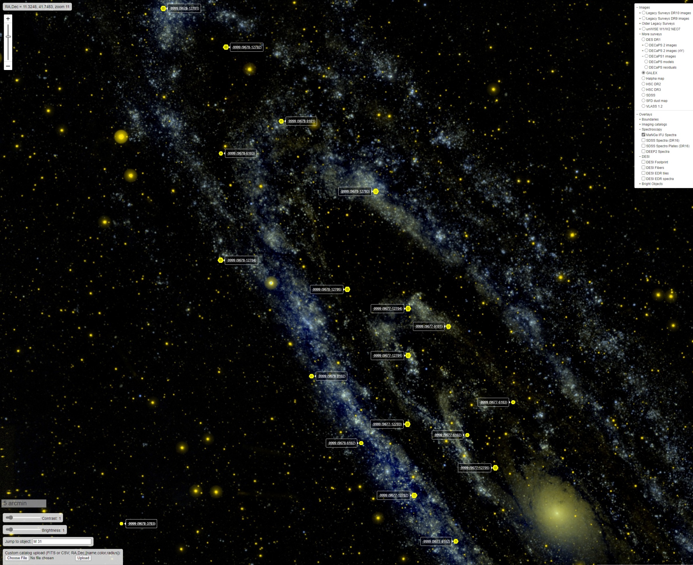
For orientation here’s a screencap of the Legacy Survey sky browser’s false color GALEX image of the northern half of M31 with the IFU positions overlaid and labelled with MaNGA’s plateifu identifiers. As a reminder these are all located within the PHAT survey footprint and specifically within the region for which star formation histories were estimated by Williams et al. (2017).
Screen capture of Legacy Survey Galex image of M31 with MaNGA IFU overlay
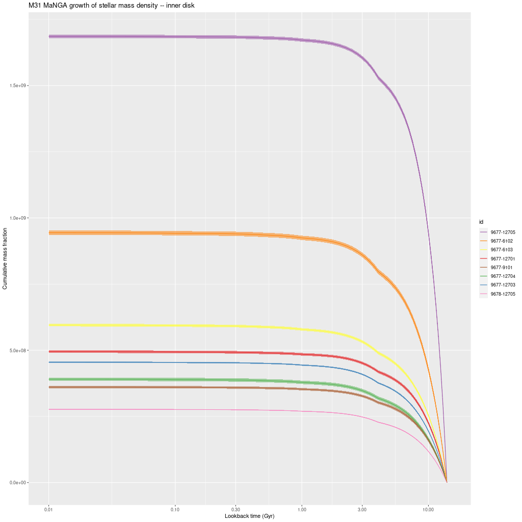
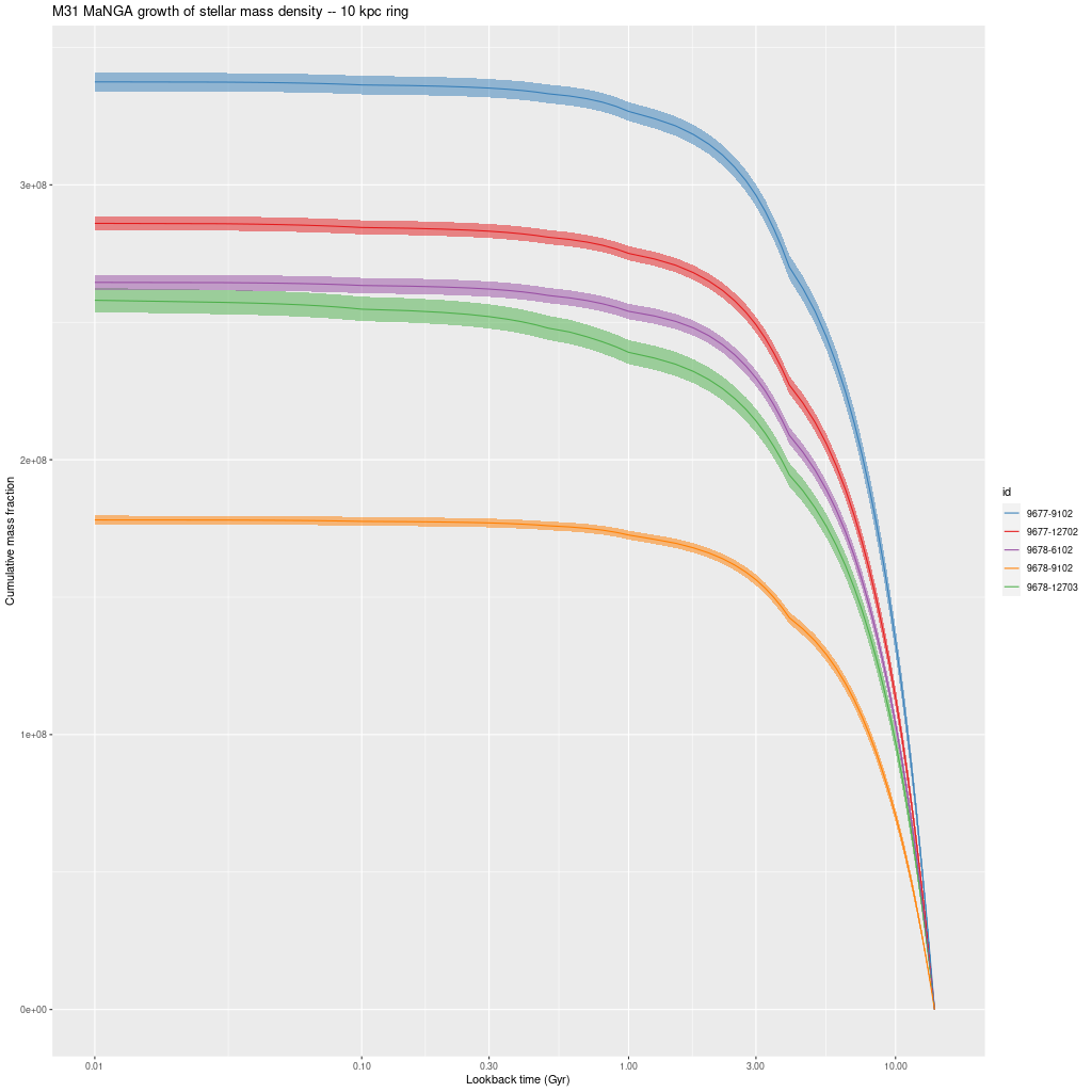
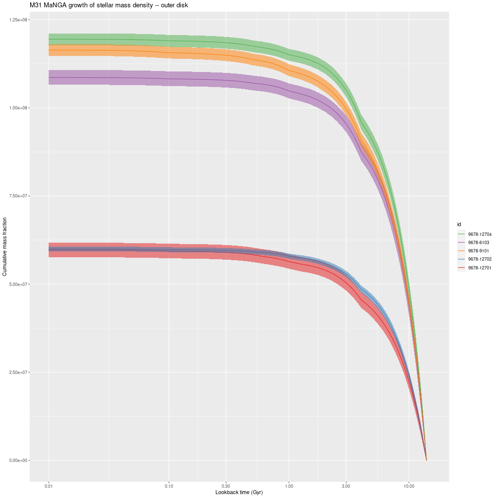
Before getting to individual IFU’s here is one more set of IFU-wide results. The following three graphs are model mass growth histories in units of present day solar mass per kiloparsec2. These are uncorrected for projection effects.
There are a couple interesting points here. There’s a clear stratification of mass density with projected radius, with about a factor 30 decline from the innermost to outermost IFU. This is in fairly good agreement with Williams’ estimate in their Figure 14.
The other thing to note is that all regions had most (> 55%) of their stellar mass in place by 8 Gyr ago and 92-99% in place by 1 Gyr ago. The largest fraction of recent star formation is in the IFU 9678-12703, which is very close to the region with the highest SFR in this half of the galaxy. There is also a trend towards later mass build up with increasing radius, which is completely consistent with the “inside-out” growth paradigm. The outermost IFU, 9678-12701 at about 16kpc radius has formed about 5% of its present day stellar mass in the past Gyr.
As I said in the previous post I don’t see clear evidence for a widespread burst of star formation that’s widely believed to have occurred around 2-4 Gyr ago. A confounding factor in my models is that they invariably show jumps in SFR at times when the interval between SSP model ages change and the two oldest of these occur at 1 and 4 Gyr, so this produces a possibly spurious period of apparently accelerated star formation. I hope to find (or perhaps produce) a set of SSP models with a better age distribution this year.
Growth of stellar mass density – inner disk M31 MaNGA IFU’sGrowth of stellar mass density – M31 MaNGA IFU’s in 10 kpc ringGrowth of stellar mass density – outer disk M31 MaNGA IFU’s
I think I’m going to hit publish now and resume with inner disk IFU’s next time.
In this post I’m going to compare IFU wide star formation histories from my models to those of Williams et al. (2017) in the nearest 83″ by 83″ PHAT tile to each MaNGA IFU in the study. I picked the Williams paper for comparison mostly because it’s possible to! They give a complete tabulation of model results for all regions and all 4 sets of isochrones that they used, and these are available through the Vizier service. Specifically I used their Table 2, which provides star formation rate densities summed over all metallicities. Since the SSP model spectra I use are based on BaSTI isochrones I initially compared to their BaSTI based models. One problem with the Williams comparison is the authors had a very wide youngest time bin of 300 Myr, which is where my models should generally have the highest precision (I make no strong claims about accuracy). It would be nice to do a similar comparison to the earlier companion paper on recent star formation by Lewis et al., which gives a much finer grained view of the last ~half Gyr, but unfortunately there is no published tabulation of their results.
At the other end of the timeline the oldest bin is also very wide, from 8 to 14 Gyr lookback time. This isn’t a surprise: the limits for reliable photometry of individual stars were rather shallow, no fainter than m = 28 or Mg ≈ 3.6 according to Lewis. This is brighter than the main sequence turnoff at 8 Gyr, so any information about the truly ancient star formation history is coming from giant branch stars which have very similar evolutionary tracks at old ages1Checked by downloading a few isochrones from the BaSTI website.
At the end of my last post I mentioned the necessity to correct densities for the rather large inclination of M31’s disk. It turns out though that I reproduce Williams’ Table 3 from their Table 2 if the densities are uncorrected. Their tabulated SFR densities are in units of 10-4 M☉arcmin-2/year. One arcminute at their adopted M31 distance is about 0.227 kpc, so to convert to star formation rates per kpc2 the values in table 2 are multiplied by 19.8 × 10⁻⁴. From my models I sum the star formation rates over all modeled spectra in each IFU and divide by the total area in fibers, with each fiber covering a projected area of 42.78 pc2. Note that I do not try to analyze a single composite spectrum summed over the entire IFU since dust attenuation is quite patchy.
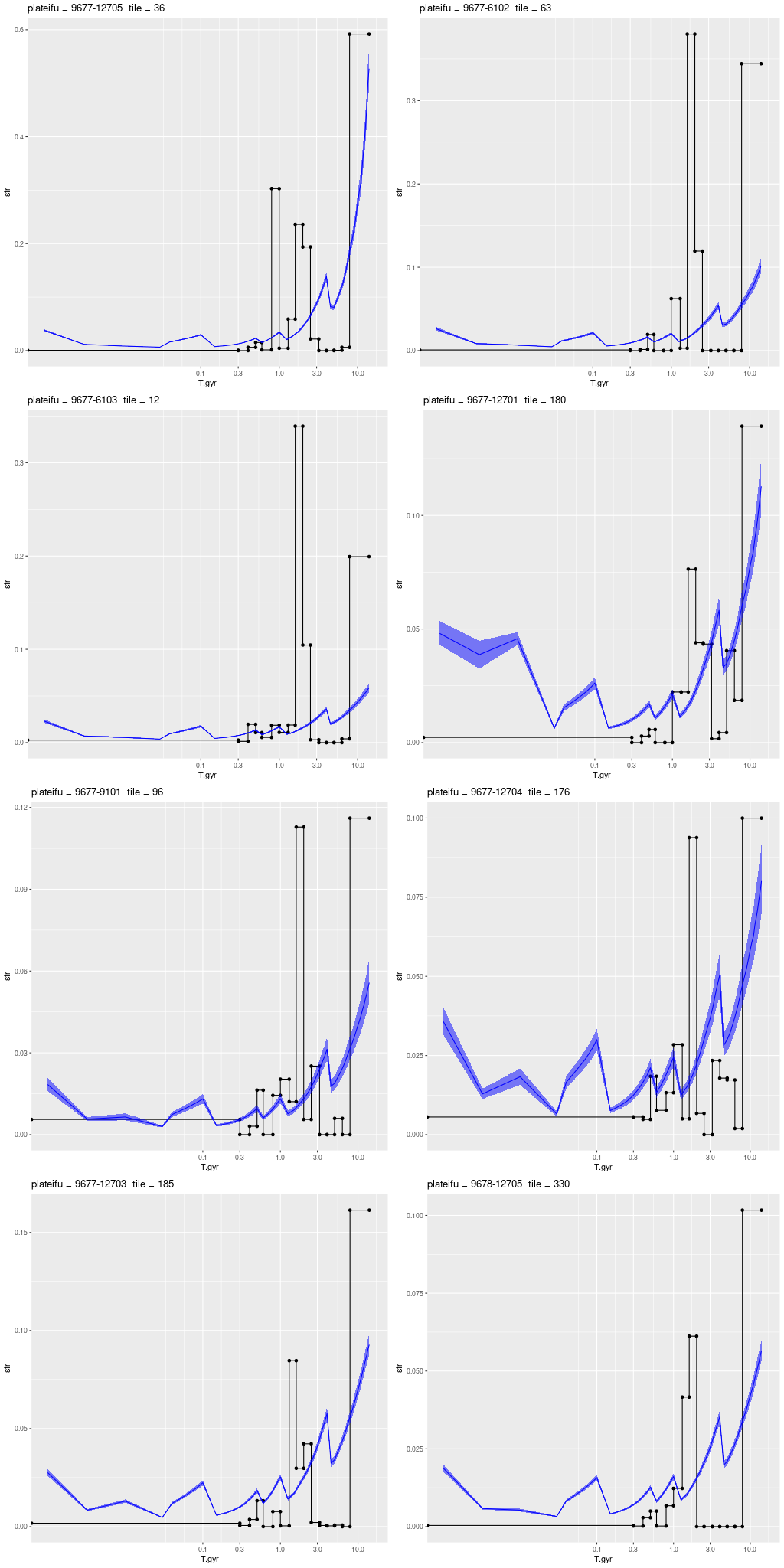
The graphs below overlay my modeled star formation rate densities on those of Williams in the tile with the nearest center to that of each IFU. The ribbons indicate the nominal 95% credible limits of SFR. These are certainly wildly optimistic. Table 2 of the paper includes uncertainty estimates, which I chose not to include. SFR densities are linearly scaled with different limits for each plot. The time scale is logarithmic. Something in between linear and logarithmic would seem more appropriate since this perhaps gives too much space to very recent times, but I haven’t found a suitable scaling.
These are ordered into three groups by location: the inner disk which is everything inside the 10 kpc ring, the 10 kpc ring, and the outer disk which is everything outside the 10 kpc ring. There’s some ambiguity about the locations of the plateifu’s 9678-9101 and 9678-12704. The first of these is about 12 kpc from the nucleus in what could be either a wide section of the 10 kpc ring or a separate structure. 9678-12704 appears in projection to be just outside the 10 kpc ring but it may be considerably farther out in a segment of spiral arm at ~15 kpc.
Commentary will continue after the graphs. I will discuss the individual IFU’s in more detail in later post(s).
Inner Disk
M31 MaNGA ancillary program – my star formation history models summed over each IFU compared to nearest tile in Williams et al. (2017) with BaSTI isochrones. Inner disk IFU’s.
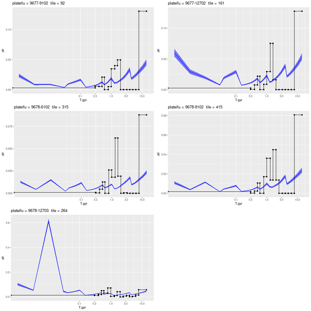
10 Kpc ring
M31 MaNGA ancillary program – my star formation history models summed over each IFU compared to nearest tile in Williams et al. (2017) with BaSTI isochrones. 10 kpc ring IFU’s.
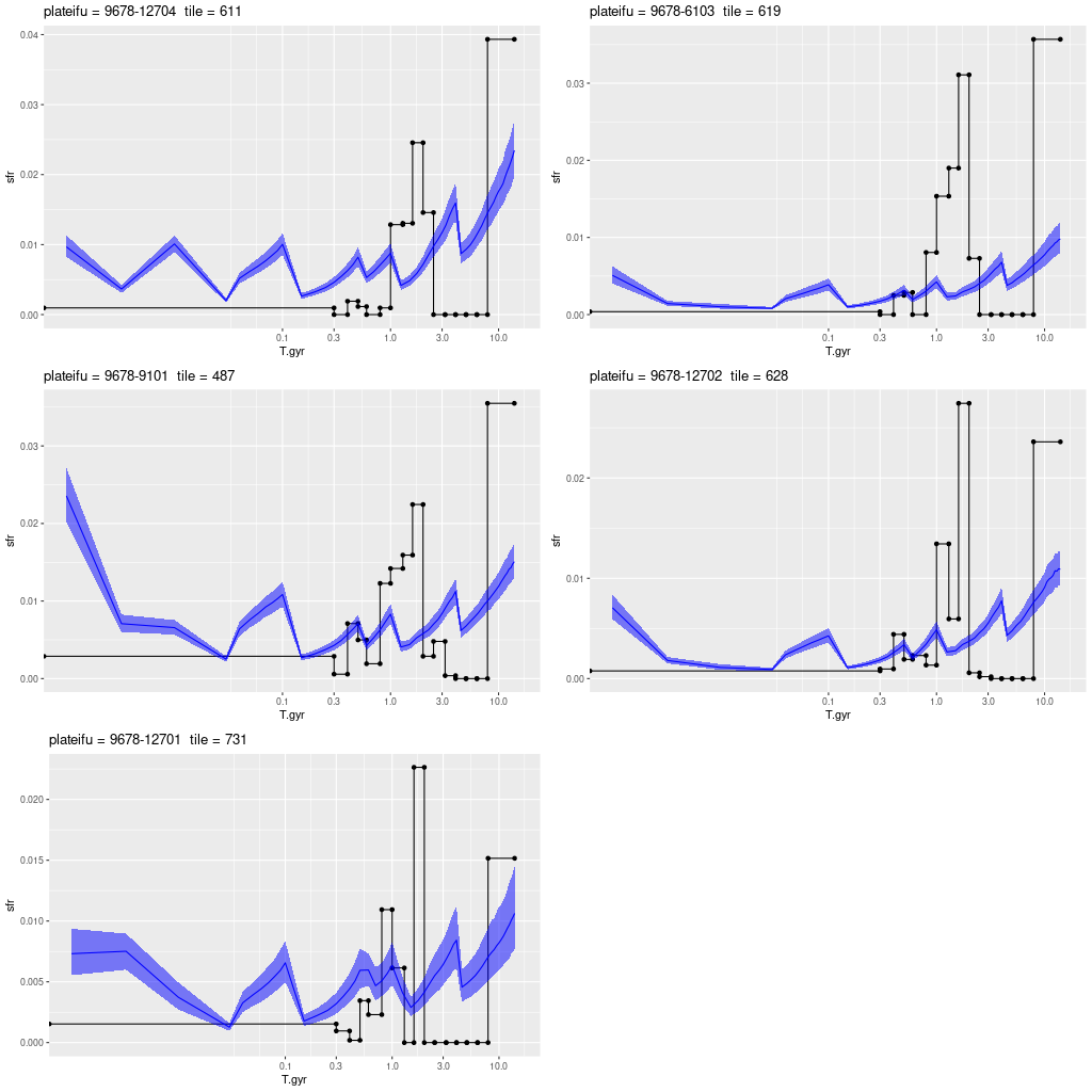
Outer disk
M31 MaNGA ancillary program – my star formation history models summed over each IFU compared to nearest tile in Williams et al. (2017) with BaSTI isochrones. Outer disk IFU’s.
The first two things I noticed were that star formation in every region declines monotonically from very early times to at least 4 Gyr ago. It also starts out lower than in the PHAT team’s models. Because of this early time mass deficit all of my models have smaller current day stellar mass densities by varying amounts. I don’t really have a pat explanation for this. Some authors have posited a “dazzle effect”2I’m going to discuss this a little further at the end of the post where recent star formation obscures the contribution of old populations. It’s certainly likely that this occurs, but if these Bayesian models are behaving as I hoped this lack of information should manifest as larger uncertainties rather than a systematic bias. Well, my hope could be wrong. On the other hand I don’t see strong evidence in these models for such an effect. From my eyeball analysis I don’t see an obvious correlation between present day star formation and the size of the early time deficit.
Another possibility is a systematic difference in the amount or shape of attenuation between my models and theirs. There is another well known “degeneracy” between stellar age and attenuation in SFH modeling, but I haven’t yet investigated whether this could be occurring here.
The PHAT models have a very long interval from 8 to ~2-3 Gyr ago with very little star formation. Some authors find evidence for a large increase from about 2-4 Gyr which is usually attributed to a merger or perhaps close encounter with M33. This isn’t seen in the BaSTI based models but there is a large more recent burst from about 1-2 Gyr lookback time. My models see neither a cessation of star formation nor a particularly large burst at intermediate ages. As I’ve noted before my models “want” to have smoothly time varying light3and therefore mass contributions and this might make a modest burst at moderately large ages difficult to discern. Another confounding factor arises from the abrupt changes in age intervals (at 0.1, 0.5, 1, and 4 Gyr) which results in the sawtooth pattern in SFR that’s obvious in every plot above.
At ages younger than 1 Gyr there’s generally good agreement about the course of star formation up until the youngest age bin of width 300Myr in the PHAT models. My models have anywhere from slightly to dramatically higher SFR densities averaged over the most recent age bin. I suspect this is because many of the IFU positions were chosen to be in regions with active star formation. In particular the plateifu 9678-12703 (mangaid 52-23) is very close to the region in the 10 kpc ring with the highest density of ongoing star formation in the northern half of the disk.
I plan to discuss the individual IFUs in more detail in a later post. Below the fold are some more graphics: mass growth histories and SFR densities compared to the PADOVA isochrone based models.