I did have my old data and model runs of course, in fact they were spread over several directories on two machines. I’m going to refer to it by this catalog designation, KUG standing for the “Kiso survey of Ultraviolet-excess Galaxies.” It’s also a low power radio source with catalog entries in both FIRST and NVSS, and of course it’s in MaNGA with plateifu ID 8440-6104 (mangaid 01-216976).
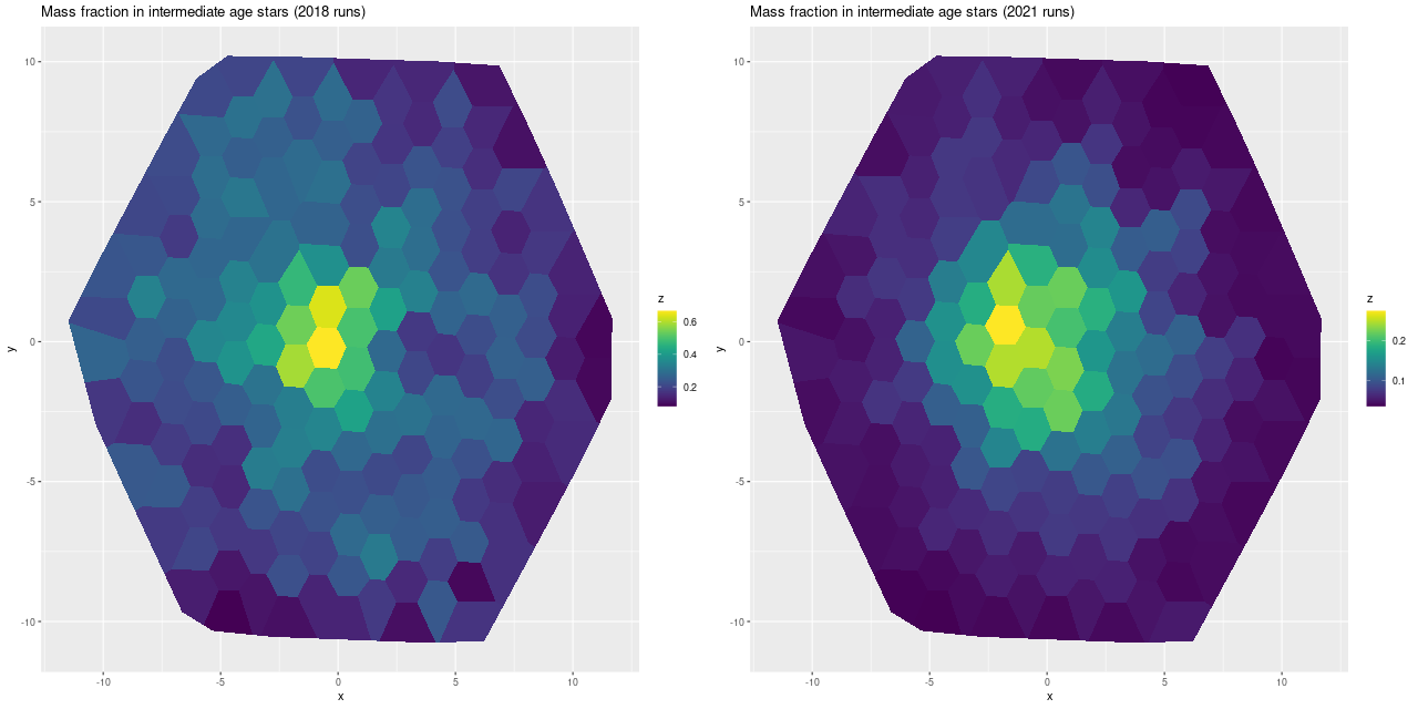
In my 2018 model runs, which were interesting enough to write 3 postsabout, I found this galaxy had undergone an extraordinarily large burst of star formation that began ~1 Gyr ago with locally as much as 60% of the present day stellar mass born in the burst and something like 40% of the mass over the footprint of the IFU. In this years model runs the peak burst fraction was a considerably more modest ~25% and globally barely amounted to a slight enhancement of star formation. The starburst was also much more localized than in the earlier runs:
Fractional stellar mass in stars between 0.1 and 1.75 Gyr old in 2018 and 2021 model runs
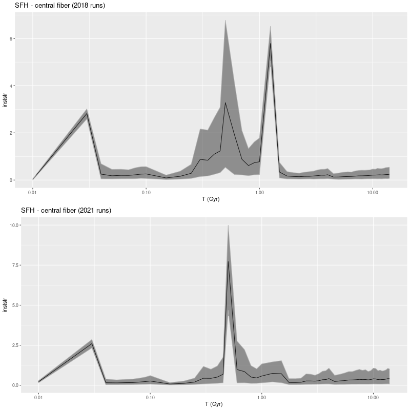
So what happened? First, here is a comparison of modeled star formation histories for the innermost fiber, which got the largest injection of mass in the starburst.
Model star formation histories for central fiber of MaNGA plateifu 8440-6104, 2018 and 2021 model runs
The obvious remark is the double peaked starburst noted back in 2018 (and discussed at some length) has been replaced with a single narrow peak with a slow ramp up and fast decay. The peak SFR is a little larger than before but the total mass in the burst is lower.
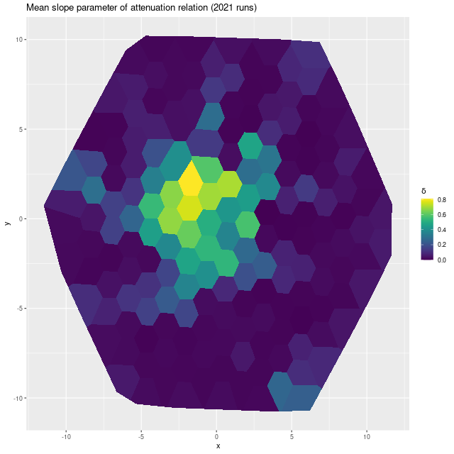
I’ve made several changes in model formulation since 2018, of which the most important in the current context is adopting the more flexible “modified Calzetti” attenuation relation that adds an additional slope parameter to the prescription. In the current year model runs a steeper than Calzetti relation is favored throughout the IFU footprint, particularly in the central region where the starburst was strongest:
Map of modified Cal;zetti slope parameter δ — MaNGA plateifu 8440-6104
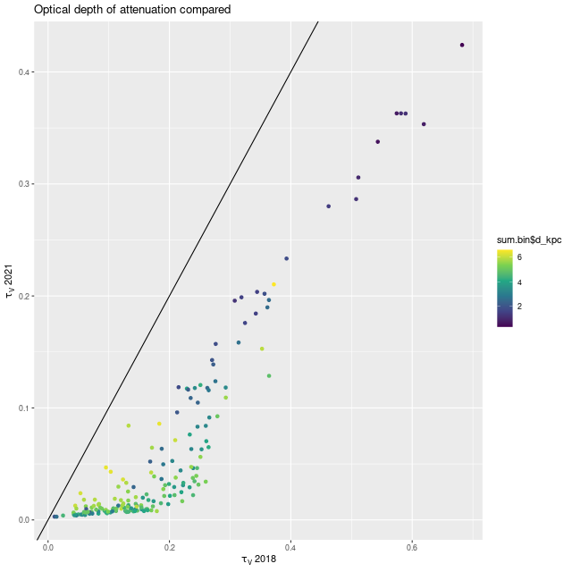
A smaller optical depth of attenuation is also favored throughout:
Modeled optical depth of attenuation – 2021 runs vs. 2018
MaNGA plateifu 8440-6104
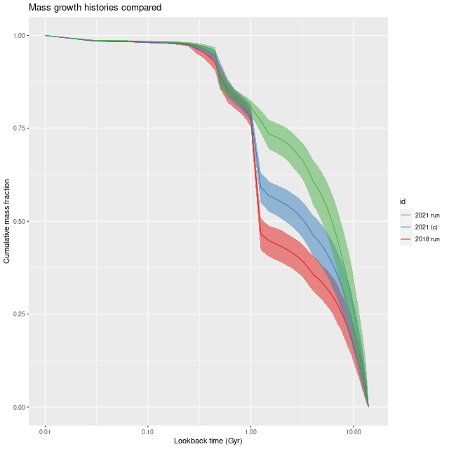
This has a couple predictable consequences. Steeper attenuation will favor an intrinsically bluer, hence younger population while a lower optical depth requires less light, and hence mass in the stellar population. I can test this directly by returning to a model with Calzetti attenuation, and here is the result for the central fiber (this model run is labeled 2021 (c) in the legend below):
Mass growth histories –
2021 run
2021 run with Calzetti attenuation
2018 run
Central fiber of MaNGA plateifu 8440-6104
So, an eyeball analysis suggests about 3/4 of the difference between the 2018 and 2021 runs is due to the modification to the attenuation relation. The other changes I’ve made to the models are to change the stellar contribution parameters from a non-negative vector to a simplex, and at the same time changing the way I rescale the data. In early runs the SSP model fluxes were scaled to make the maximum stellar contribution ≈ 1, while the current models scale both the galaxy and SSP fluxes to ≈ 1 in the neighborhood of V, making the individual stellar contributions approximately the fraction of light contributed. An additional scale factor parameter in the model is used to adjust the overall fit. Assuming I did this right this should have no effect on a deterministic maximum likelihood solution, but with MCMC who knows?
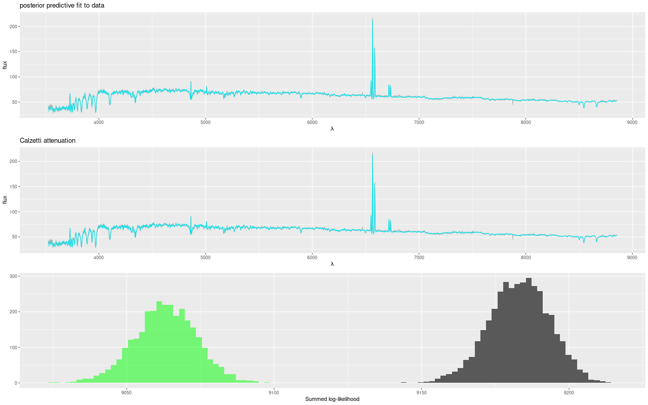
Although the fit to the data looks about the same between the model with and without the attenuation modification the summed log-likelihood is consistently about 1% higher for the modified Calzetti model with no overlap at all in the distribution of likelihood. This suggests the case for a steeper than Calzetti attenuation is a fairly robust result.
“Posterior predictive” fits to galaxy flux data – modified Calzetti attenuation vs. Calzetti – central fiber of MaNGA plateifu 8440-6104
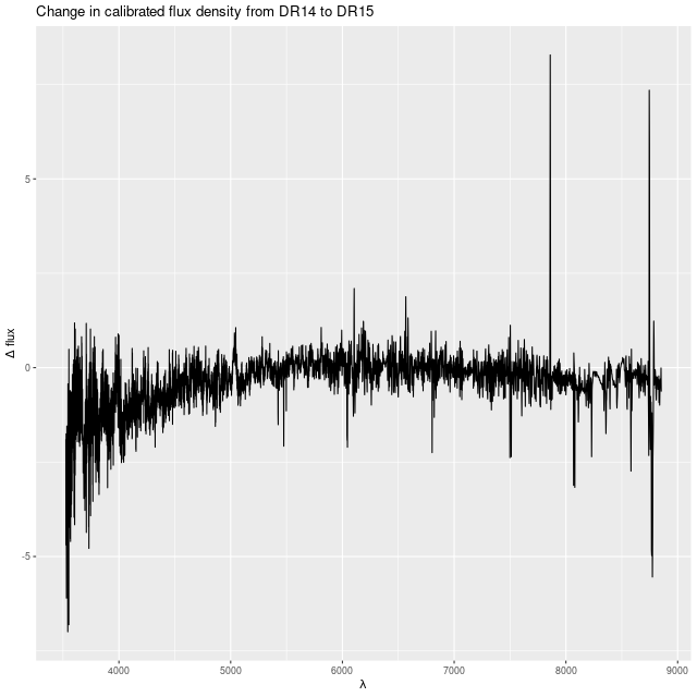
The galaxy flux data also changed a little bit. The early runs were on the DR14 release (version 2_1_2 of the MaNGA DRP) while the recent ones used the DR15 release (ver 2_4_3). Most of the calibration differences resemble random noise, but there is some curvature that systematically affects both the red and blue ends of the spectrum and could cause some change in the temperature distribution of the models:
Difference in measured flux from DR14 to DR15 – central fiber of MaNGA plateifu 8440-6104
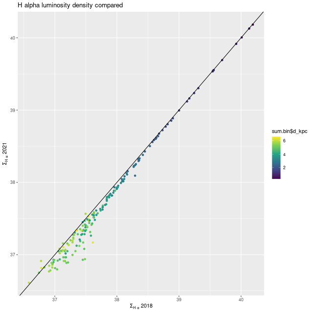
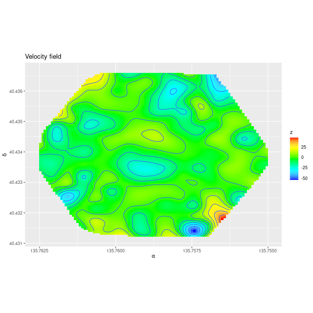
While the detailed star formation histories changed, quantities that aren’t too model dependent didn’t very much. One example is shown below. Also, the kinematic maps agree with the earlier ones in detail.
Hα luminosity density – 2021 runs vs. 2018
MaNGA plateifu 8440-6104Velocity field of MaNGA plateifu 8440-6104 from 2021 model runs. Map interpolated from RSS file spectra.
One input that hasn’t changed are the emiles SSP model spectra, although there have been some procedural changes in how I handle the modeling. Early on I often used a much smaller subset of SSP models with just 27 time bins and 3 metallicities for preliminary modeling, including my first models on the same binning of these data. I also routinely ran 250 warmup iterations with just 250 more per chain. My current standard practice is always to use the largest emiles subset with 216 SSP models in 54 time bins and 4 metallicities, and I generally run 750 post-warmup iterations per chain but still with only 250 warmup iterations. This is generally enough and if adaptation fails it is usually fairly obvious. The small sample size of the earlier runs mostly effects the precision of inferences rather than means.
To conclude for now, my speculation about whether it might be possible to say something about the timing of critical events in a merger from the model star formation history was too optimistic. On a positive note though both sets of model runs retrodict that coalescence occurred at a lookback time around 500Myr ago, which is consistent with the fact that tidal tails and other merger signatures are clearly visible even in SDSS imaging. Both sets of model runs also have that odd uptick in star formation at 30Myr in the central fiber. And while the difference in burst mass contributions is a little disconcerting the current runs are more consistent with the likely gas content of ordinary spiral galaxies.
This example illustrates another well known “degeneracy” among attenuation (and adopted attenuation relation), mass, and stellar age. Whether I’ve broken the degeneracy by adopting the more flexible attenuation prescription described some time ago remains to be validated.
This paper (arxiv ID 2103.16070) is pretty old by now, having been posted on arxiv back in early April. The basic premise of the work is mildly interesting: the author searched MaNGA for galaxies that would meet conventional criteria for post-starburst (aka K+A etc.) spectra if observed at a redshift high enough that the entire galaxy would be covered by a single fiber like the original SDSS spectroscopes. Somewhat surprisingly, he found just 9 that met his selection criteria in the DR15 sample of ~4500 galaxies.
I have to say the paper itself is forgettable, but a manageably sized sample of MaNGA data that’s complete by some criterion is worth a look, and I have a long-standing interest in post-starburst galaxies in particular. So, I ran my current SFH modeling code on all 9 — by the way this was completed some time ago. It’s just taken me a while to get around to generating some graphics and sitting down to write.
The author only measured a few observable quantities: Hδ equivalent width and the 4000Å break index Dn(4000), along with Hα emission equivalent width and (normalized) fluxes. I long ago validated my own absorption line measurements of SDSS single fiber spectra against the MPA-JHU measurement pipeline, which was the gold standard for several years (but last run on DR8). My measurements and uncertainty estimates are in excellent agreement with theirs, so I have a fair amount of confidence in them. Emission line fluxes also agree with published measurements with considerably more scatter. My emission line equivalent widths on the other hand are completely unchecked. So, one of my tasks was to compare my equivalent width measurements with Wu’s. I did not attempt to exactly reproduce his work – I binned spatially using my usual Voronoi partitioning approach whereas Wu binned in elliptical annuli. With that difference in mind the next two plots should be compared to his Figures 4 and 5.
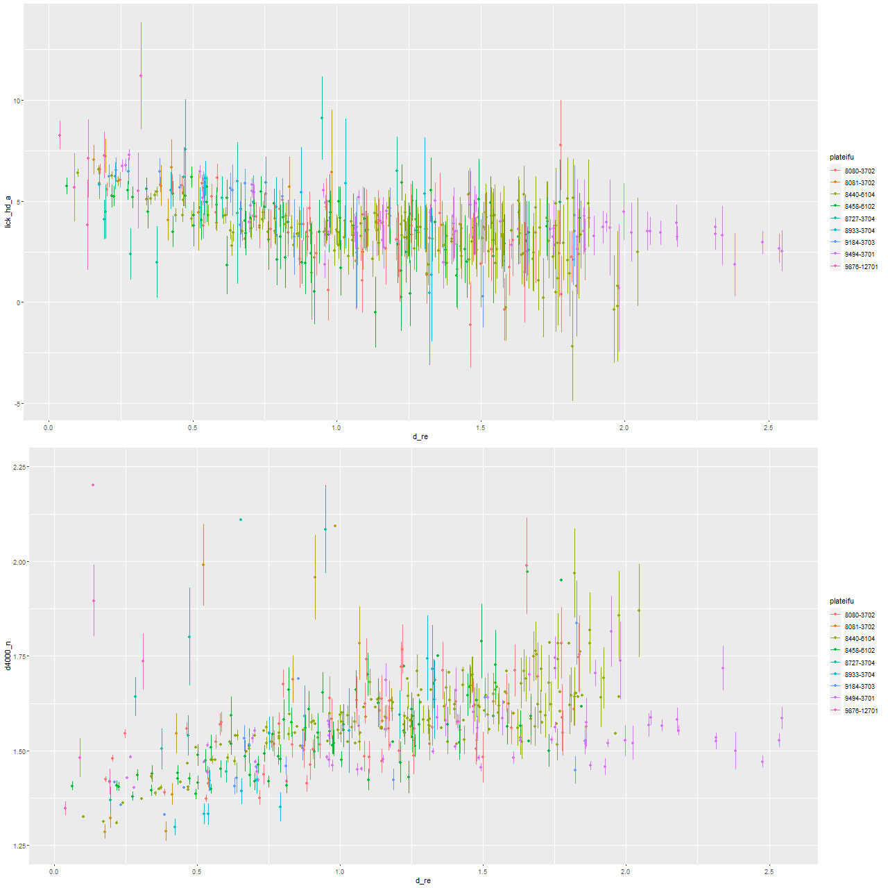
The first two graphs show the radial trends (relative to the effective radii per the NASA/SLOAN catalog) in the Lick HδA and Dn(4000) indexes. These both show very similar trends to Wu’s measurements although with more scatter. This is expected because fewer spectra go into each point in general — from the text it appears Wu binned several separate measurements for each displayed point. Also, I made no attempt to deproject distances. One feature of the Hδ versus radius plot that’s a little different is the trend generally flattens out beyond ∼1 effective radius, while Wu shows a roughly linear trend out to 1.5 Re. This might just be a visible effect of me displaying the trends out to larger radii.
Radial trends of Lick HδA and Dn4000 for 9 MaNGA “post-starburst” galaxies from Wu (2021) – arxiv 2103.16070
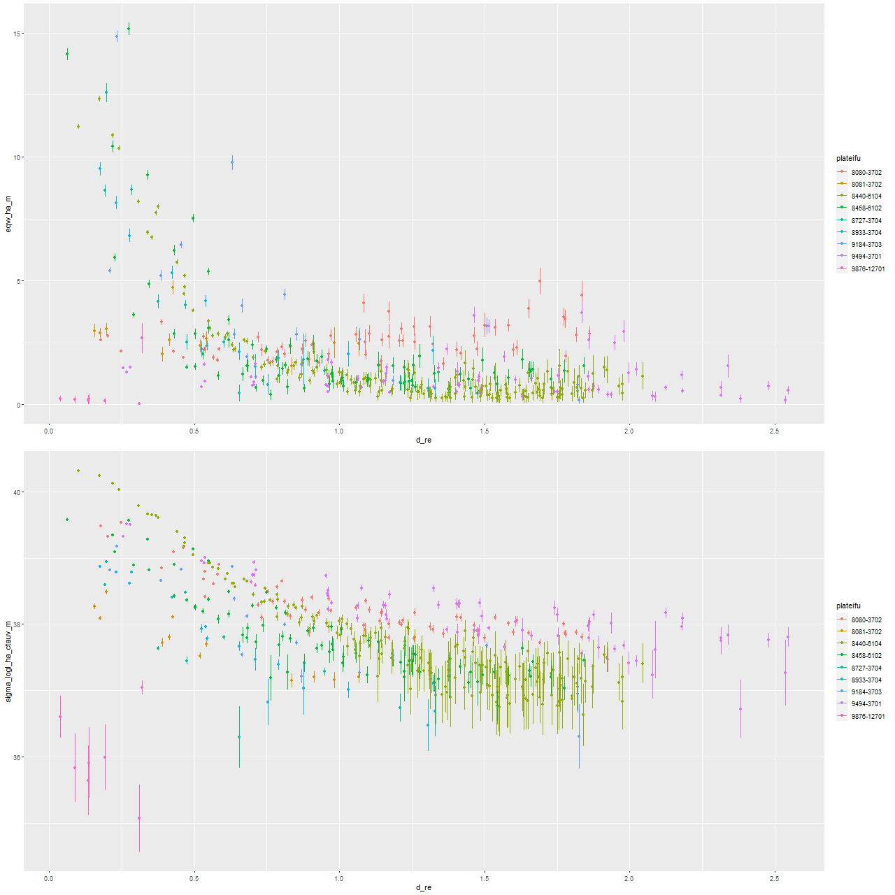
The Hα emission line measurements are similarly in broad agreement. Like Wu, I find that there are two distinct trends in emission: either moderately strong centrally with a rapid decline or weak throughout with a relatively flat trend. One galaxy (with MaNGA plateifu 9876-12701) has no detectable emission. I haven’t looked in detail at emission line ratios to compare to Wu’s Figure 7, but there’s general agreement that some residual star formation is present in some of the sample and weak AGN or ionization by hot evolved stars in others.
Radial trends of Lick Hα equivalent width and luminosity density for 9 MaNGA “post-starburst” galaxies from Wu (2021) – arxiv 2103.16070
A fairly common failing of this literature (IMO) is the use of proxies for recent star formation but not attempting actually to model star formation histories. There are plenty of publicly available tools for that available now, so there’s really no reason not to perform such modeling exercises. Wu did do some toy evolutionary modeling and posted a graph of trajectories through the Hα emission – Hδ absorption plane, which can scarcely unambiguously constrain star formation histories. Of course much of my hobby time is spent generating fine grained model star formation histories, so let’s take a look at a few selected results.
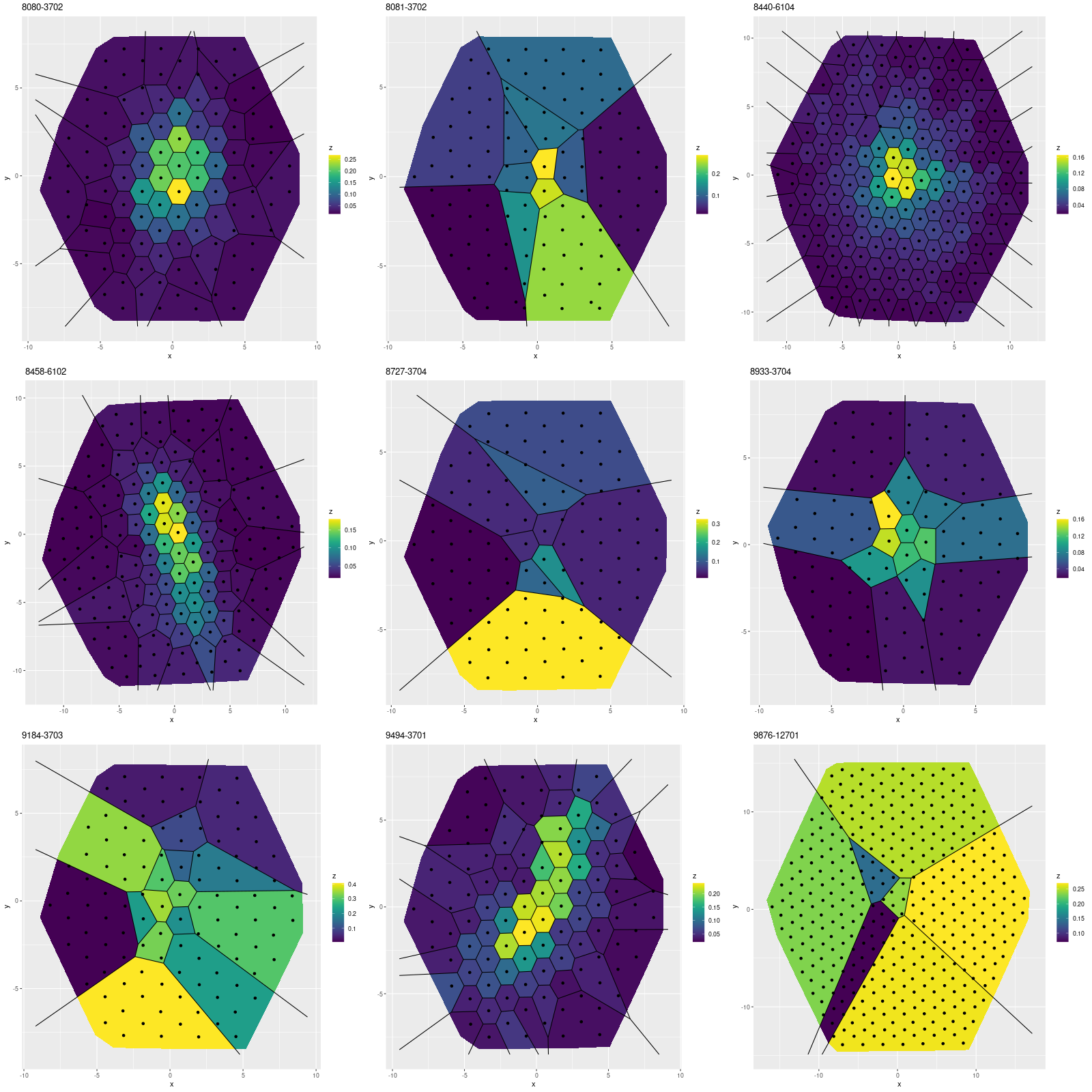
First, here are maps of the modeled fraction of the current stellar mass in stars of ages between 0.1 and 1 Gyr, very roughly the age range that produces a post-starbursty spectrum. Six of the galaxies have more or less strongly centrally concentrated intermediate age populations, which is generally what’s expected especially in the major merger pathway to a post-starburst interval. I’ll discuss this a little further below.
Maps of fractional stellar mass in intermediate age populations for 9 MaNGA “post-starburst” galaxies from Wu (2021) – arxiv 2103.16070
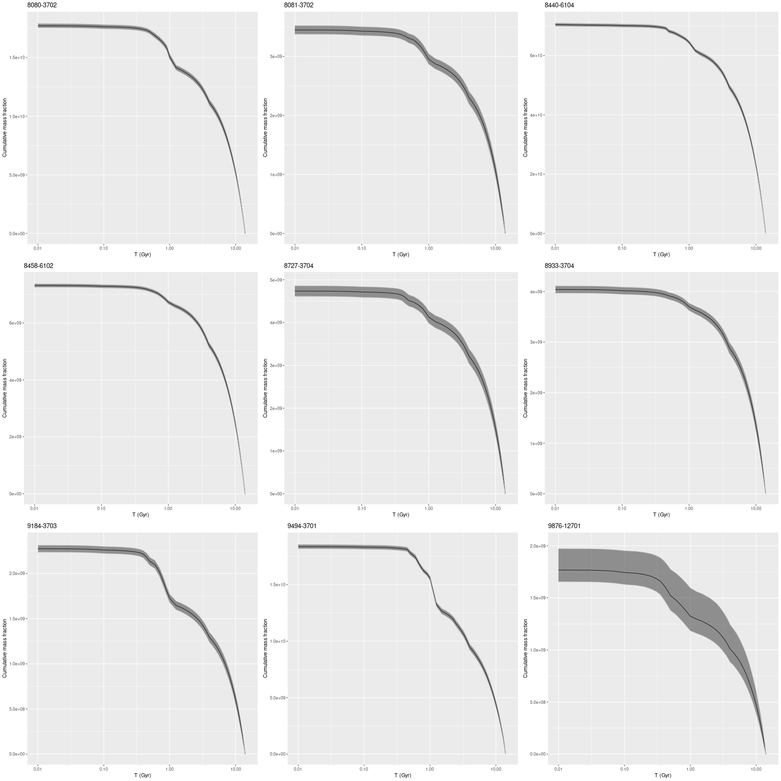
In more detail here are summed mass growth histories for the sample, that is all modeled star formation histories for a given observation are summed to produce a single global estimate. I’ve shown total masses here. Because of the pointing strategy MaNGA uses the fiber positions overlap to produce a 100% filling factor, so simply summing overestimates masses by about 0.2dex according to a calculation I performed some time ago. The present day masses in the plot below actually agree pretty well with the values listed in Table 1 of the paper, with an average difference of ~0.1 dex (this is probably because at least some of the light falls outside the IFU footprint in most of these galaxies, offsetting some of the overcounted mass).
Integrated mass growth histories for 9 MaNGA “post-starburst” galaxies from Wu (2021) – arxiv 2103.16070
Somewhat surprisingly several of these galaxies show little evidence of an actual burst of star formation in the recent past, at least at the global level. Some of these could simply have had star formation truncated recently, which can produce a poststarburst spectral signature for a time. Overall intermediate age stars contribute ~ 6-20% of the present day stellar mass, with the two largest contributions in the low mass galaxies in the bottom row of the plot.
There are some other oddities in this small sample. At least 3 galaxies are dwarf ellipticals or perhaps dwarf irregulars (in the case of plateifu 9876-12701), and two others have stellar masses under ~5 x 10⁹ M⊙. Two of the low mass galaxies are in or near the Coma cluster, which suggests environmental effects as the probable cause of quenching. Another possible issue with the low mass galaxies is the infamous “age-metallicity degeneracy,” which refers to the fact that old, low metallicity populations “look like” younger, more metal rich ones by many measures. The Balmer lines in particular fade more slowly with age in lower metallicity populations, and the 4000Å break also becomes metallicity sensitive (smaller at low metallicities) at older ages.
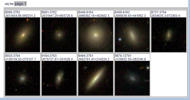
There is only one clear merger remnant in the sample (with plateifu 8440-6104, which I will get to in a moment). One other galaxy (plateifu 8458-6102) is located in a compact group that appears (in Legacy survey imaging) to be embedded in a cloud of extragalactic light. Finally, two galaxies in this sample have been cataloged as K+A based on SDSS spectra — 8080-3702 and 9494-3701, while two others in the catalog of Melnick and dePropris (2013) are not.
SDSS thumbnails of the sample
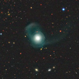
The one clear merger remnant in the sample is an old friend of mine, and in fact I wrote three lengthy posts about this one back in 2018. In perusing those posts I noticed that the current set of model runs have a slightly weaker and more recent burst than the earlier runs. Also a double peak in the earlier runs has gone away in these, which means my early speculation that it might be possible to time crucial events in a merger from the detailed SFH model was too optimistic. On the other hand the model burst strength in the earlier runs was uncomfortably large, indicating an exceptionally gas rich merger and efficient processing of gas into stars. The current runs have a more reasonable ~10% of mass in the burst. So, I will look into those earlier runs and try to figure out what changed. Fortunately I’m a data hoarder and R is self-archiving to some extent.
KUG 0839+406, one of 9 “post-starburst” galaxies in Wu (2021)
The idea of looking at the integrated properties of IFU data to pick a post-starburst sample seems reasonable, but this sample appears to me to be both incomplete and possibly with some false positives. When DR17 is finally released I plan to try to develop my own criteria. As I’ve already shown using SDSS spectra alone to select a sample is doomed to produce lots of false positives.
I should finally mention one other paper pursuing a similar idea by Greene et al. (2021) showed up on arxiv recently. The authors lost me when they used the phrase “carefully curated” in their introduction, which was otherwise pretty well written up to that point. Maybe I’ll take another look anyway.
I decided to try a set of models for one galaxy – NGC 4889 (with MaNGA plateifu 8479-12701), which had the highest overall velocity dispersion of the Coma sample I’ve been discussing in the last several posts. It also has some evidence for multiple kinematic components which isn’t too much of a surprise since it’s one of the central cD galaxies in Coma. The SSP model spectra fed to the SFH models were preconvolved with the element wise means of the LOSVD convolution kernels from the velocity distribution modeling exercise. Again, this is an expedient to avoid what could otherwise be prohibitively computationally expensive. The models I ran were the same as described back in this post — these ignore emission but do model dust attenuation with the usual modified Calzetti attenuation relation.
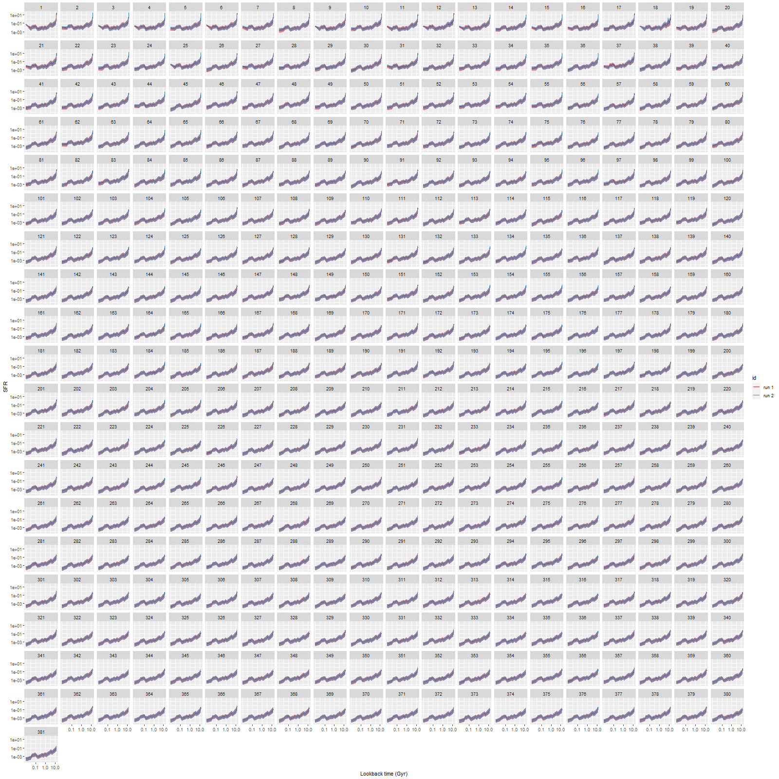
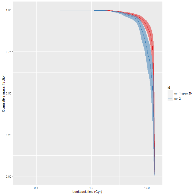
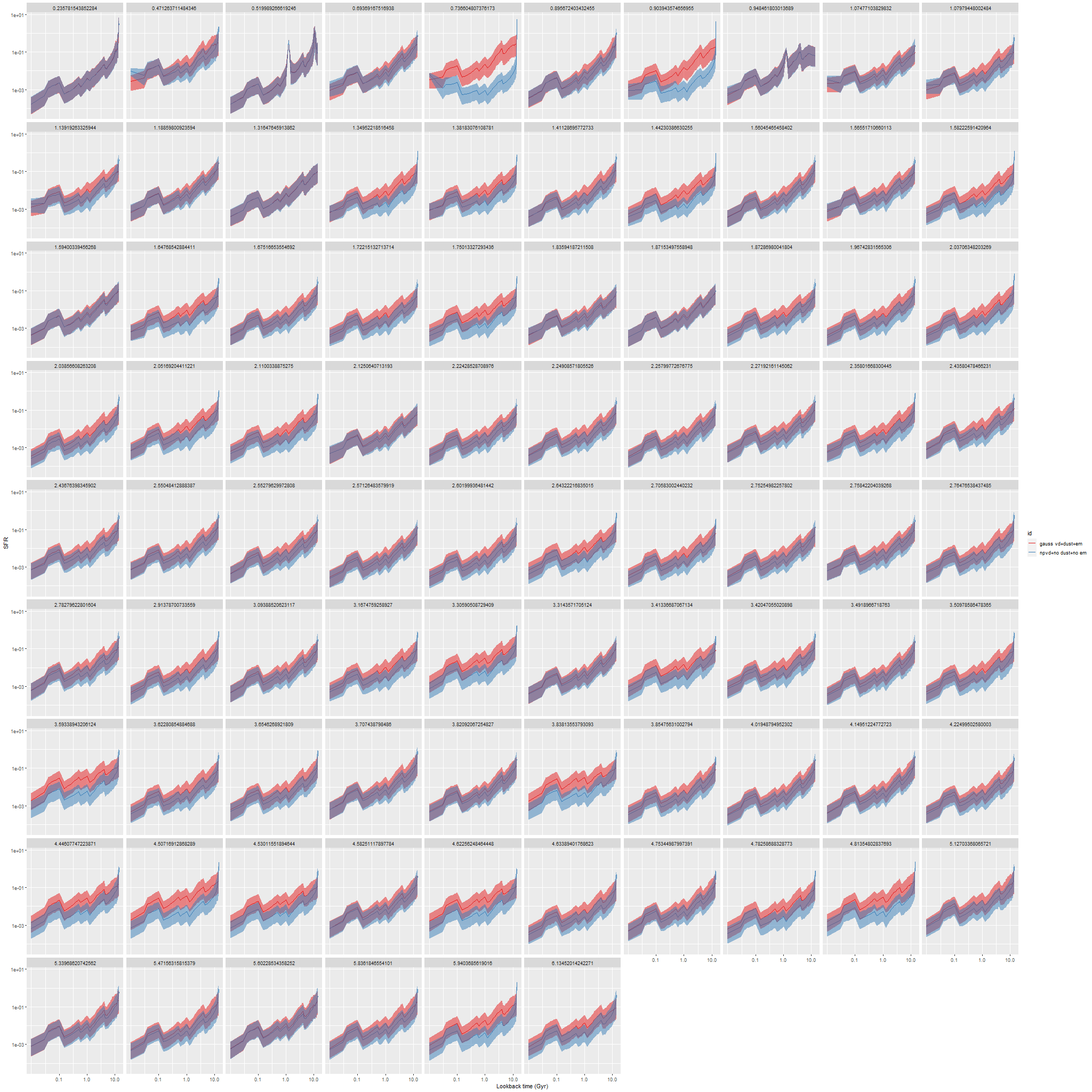
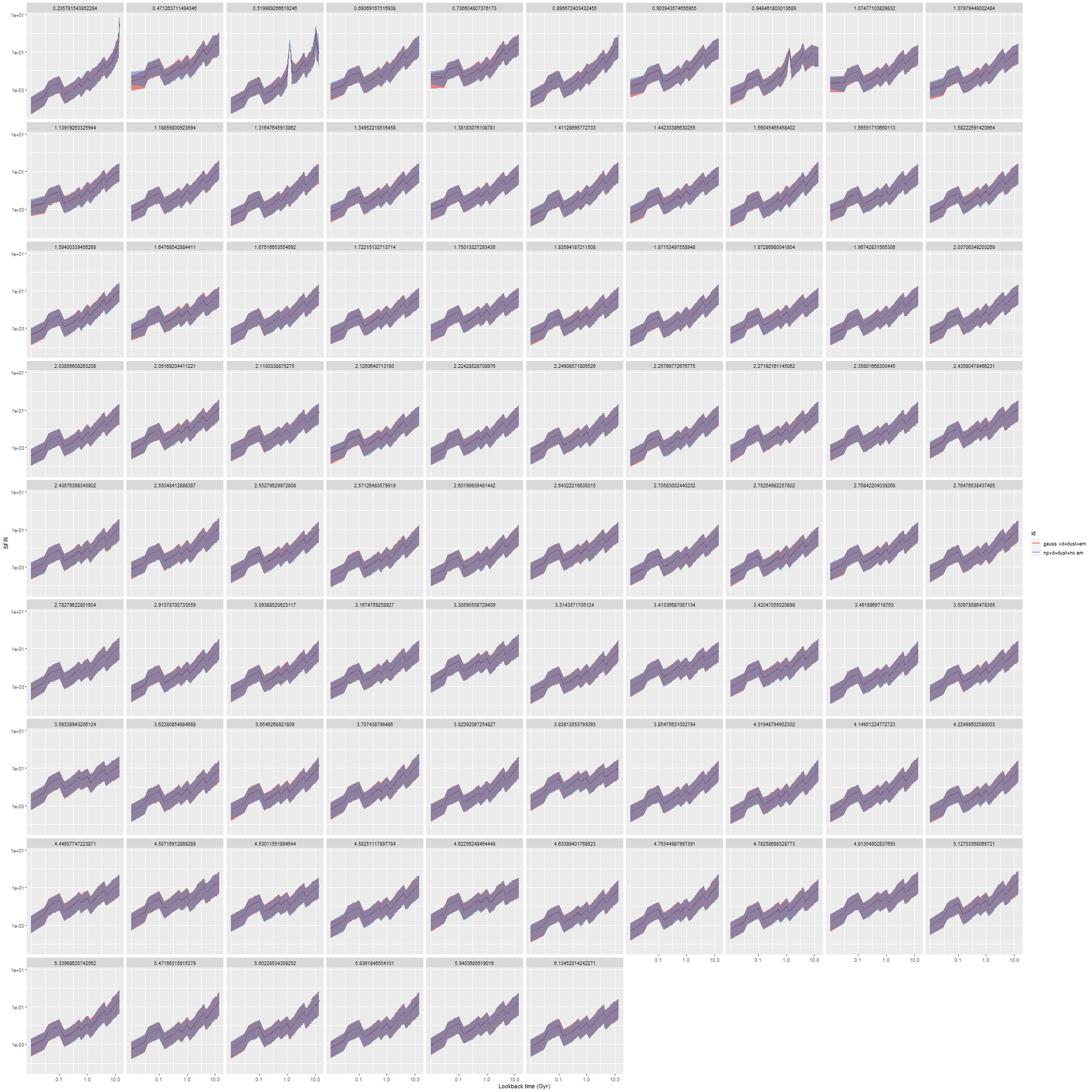
To get quickly to the results, here are model star formation histories compared to the previous runs that used the full model in its current form. Usually I like these plots of results from all spectra in an IFU, but in this one all 381 spectra met my S/N criterion, so the plot is pretty crowded. You really need to see it live on a 4K monitor to see the details.
NGC 4889 (MaNGA plateifu 8479-12701)
Model star formation histories for all spectra, runs with non-parametric LOSVD vs. single gaussian stellar velocity dispersions
Well it’s pretty hard to see but differences in model SFH’s are mostly in the youngest age bins, which are very poorly constrained anyway in these presumably passively evolving galaxies. Here’s a closer look at a single model run that had the largest difference in estimated stellar mass density (more on this right below) of about 0.19 dex:
NGC 4889 (MaNGA plateifu 8479-12701)
Model mass growth histories for a single spectrum – runs with non-parametric LOSVD vs. single Gaussian stellar velocity dispersion
So, the difference in star formation histories was slower mass build up between about 12-5 Gyr look back times in the second run, which was responsible for the lower current day stellar mass density. How this resulted from the choice of LOSVD is not at all obvious.
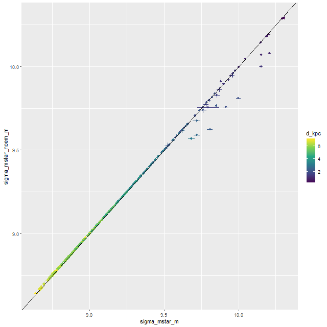
Let’s look at a few summary results. First, the model stellar mass surface densities:
NGC 4889 (MaNGA plateifu 8479-12701)
Model ΣM* – runs with non-parametric LOSVD vs. single Gaussian stellar velocity dispersion
These fall on an almost exactly one to one relation with a few hands full of outliers. Oddly these are mostly in the higher signal to noise area of the IFU (i.e. near the center).
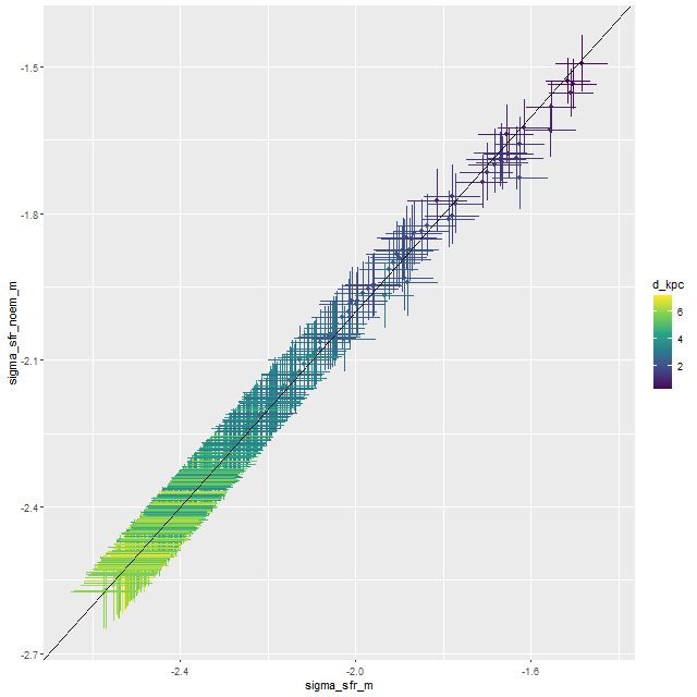
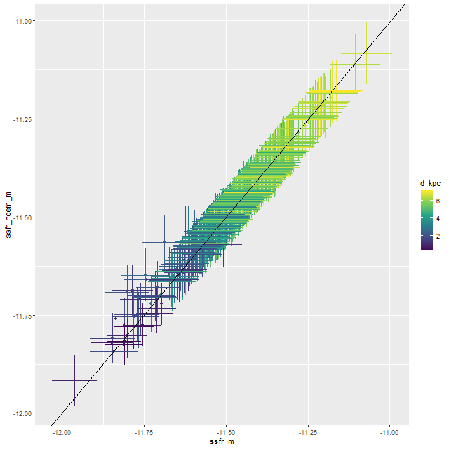
Results for star formation rate density and specific star formation rate are even more consistent between runs, with essentially no differences larger than the nominal 1 σ error bars.
NGC 4889 (MaNGA plateifu 8479-12701)
Model Σsfr – runs with non-parametric LOSVD vs. single Gaussian stellar velocity dispersionNGC 4889 (MaNGA plateifu 8479-12701)
Model SSFR – runs with non-parametric LOSVD vs. single Gaussian stellar velocity dispersion
One problem I encountered was that I had to re-run some models either for technical reasons or because of obvious convergence failures. I suspect there could have been some convergence issues in both sets of runs and am slightly worried that could be the source of the few differences in summary measures seen. Oddly, there were almost no suspicious convergence diagnostics in either set of runs (once the latter were run to satisfactory conclusion), and Stan is quite aggressive about reporting possible convergence issues.
Anyway, modeling kinematics remains an interesting topic to me, but it seems somewhat decoupled from modeling star formation histories. Right now I’m waiting for the final SDSS data release to decide what projects I want to tackle.
I’m going to end with a couple of asides. First, I recognize that all of these error bars are overoptimistic, maybe by a lot. The main reason, I think, is that I treat the flux values as independent which they clearly are not1 this is pretty standard practice however, which effectively results in overestimating the sample size. One possible partial solution is to allow the flux uncertainties to vary from their nominal values by, for example, a factor > 1. This would involve adding as few as one parameter to the models, which is something I’ve actually tried in the past. I may relook at that.
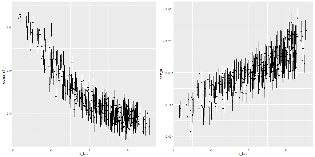
One interesting feature of the previous two graphs is the rather obvious systematic trend with radius of both SFR density and specific star formation rate, as shown more directly below taken from the first set of model runs:
NGC 4889 (MaNGA plateifu 8479-12701)
ΣSFR and SSFR vs. distance from IFU center
Are these real trends? I don’t know, but I don’t see an obvious reason why they might be spurious features of the models. In normal star forming galaxies I encounter trends with radius in both directions and sometimes no trend at all.
As a final and related aside there was a paper by Sedgwick et al. that showed up on arxiv not long ago that presented estimates of star formation rates of early type galaxies from observations of core collapse supernovae carefully matched to host galaxies with high confidence morphological classifications. To oversimplify their conclusions they found that typically massive ellipticals might have specific star formation rates ∼ 10-11 / yr, which is somewhat higher than usually supposed. As I mentioned in my last post my models will always have some contribution from young stars and I typically get central estimates of SSFR > ∼ 10-11.5 even in galaxies with no hint of emission (as is the case with this Coma sample). This particular galaxy has a total stellar mass within the IFU of ∼ 1011.5 M⊙ , so it could be forming stars at a rate of ∼ 1 M⊙ / yr.
Well, I think I have one more post to write before the SDSS DR17 release.
I’ve posted versions of some of these graphs before for both individual galaxies and a few larger samples, but I think they’ve all been unusual ones. I recently managed to complete model runs on 40 of the spirals from the normal barred and non-barred sample I discussed back in this post. The 20 barred and 20 non-barred galaxies in the sample aren’t really enough to address the results in the paper by Fraser-McKelvie that was the starting point for my investigation and more importantly the initial sample was chosen entirely at my whim. Unfortunately I don’t have the computer resources to analyze more than a small fraction of MaNGA galaxies. The sampling part of the modeling process takes about 15 minutes per spectrum on my 16 core PC (which is a huge improvement) and there are typically ~120 binned spectra per galaxy, so it takes ~30 hours per galaxy with one PC running at full capacity. I should probably take up cryptocurrency mining instead.
This sample comprises 5086 model runs with 2967 spectra of non-barred and 2119 of barred spirals. For some of the plots I’ll add results for 3348 spectra of 33 passively evolving Coma cluster galaxies.
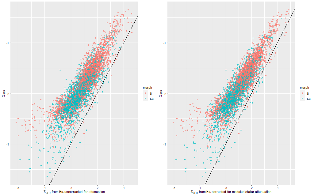
Anyway, first: the modeled star formation rate density versus the rate predicted from the Hα luminosity density, which is easily the most widely used star formation rate calibrator at optical wavelengths. The first plot below shows all spectra with estimates for both values. Red dots are (non-barred) spirals, blue are barred. Both sets of quantities have uncertainties calculated, but I’ve left off error bars for clarity. Units on both axes are log10(M☉/yr/kpc2). I adopted the relation log(SFR) = log(LHα) – 41.26 from a review by Calzetti (2012), which is the straight line in these graphs. That calibration is traceable back to Kennicutt (1983), which as far as I know has never been revisited except for small adjustments to account for changing fashions in assumed stellar initial mass functions. In the left panel of the plot below Hα is uncorrected for attenuation. In the right it’s corrected using the modeled stellarattenuation, which as I noted some time ago will systematically underestimate the attenuation in H II regions. Not too surprisingly almost all points lie above the calibration line — the SFH models include a treatment of attenuation that might be too simple but still does make a correction for starlight lost to dust. The more important observation though is there’s a pretty tight relationship between modeled SFR density and estimated Hα luminosity density that holds over a nearly 3 order of magnitude range in both. The scatter around a simple regression line in the graphs below is about 0.2 dex. It’s not really evident on visual inspection but the points do shift slightly to the right in the right hand plot and there’s also a very slight reduction in scatter. These galaxies are actually not especially dusty, with an average model optical depth of around 0.25 (which corresponds to E(B-V) ≈ 0.07).
SFR density vs. prediction from Hα luminosity for 40 normal spirals.
(L) Hα luminosity uncorrected for attenuation.
(R) Hα corrected using estimated attenuation of stellar component.
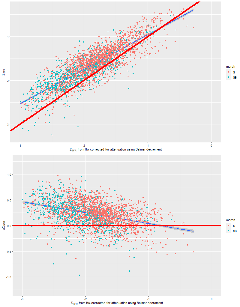
To take a more refined look at this I limited the sample to regions with star forming emission line ratios using the standard BPT diagnostic based on [O III]/Hβ vs. [N II]/Hα. I require at least a 3σ detection in each line to make a classification, so besides limiting the analysis to regions that are in fact (I hope) forming stars it allows correcting Hα attenuation for the observed Balmer decrement since Hβ is by construction at least nominally detected. Now we get the results shown in the plot below. Units and symbols are as before. Hα luminosity is corrected using the Balmer decrement assuming an intrinsic ratio of 2.86 and the same attenuation curve shape as returned by the model. The SFR-Hα calibration line is the thick red one. The blue lines with grey ribbons are from “robust” simple regressions using the function lmrob in the R package robustbase1Correcting for attenuation produced a few significant outliers that bias an ordinary least squares fit and although it’s not specifically intended for measurements with errors this function seems to do a little better than either ordinary or weighted least squares.
Model estimates of star formation rate density vs. SFR predicted from Hα luminosity density.
So the model SFR density straddles the calibration line, but with a distinct tilt — regions with relatively low Hα luminosity have higher than expected star formation. To quantify this here is the output from the function lmrob:
Call:
lmrob(formula = sigma_sfr_m ~ sigma_sfr_ha, data = df.sfr)
 \--> method = "MM"
Residuals:
      Min        1Q    Median        3Q       Max
-3.862996 -0.142375  0.004122  0.137030  1.305471

Coefficients:
              Estimate Std. Error t value Pr(>|t|)
(Intercept)  -0.174336   0.019224  -9.069   <2e-16 ***
sigma_sfr_ha  0.785954   0.009948  79.008   <2e-16 ***
---
Signif. codes:  0 ‘***’ 0.001 ‘**’ 0.01 ‘*’ 0.05 ‘.’ 0.1 ‘ ’ 1

Robust residual standard error: 0.2097
Multiple R-squared:  0.7402,	Adjusted R-squared:  0.7401
Convergence in 10 IRWLS iterations

Robustness weights:
 6 observations c(781,802,933,941,2121,2330) are outliers with |weight| = 0 ( < 3.8e-05);
 223 weights are ~= 1. The remaining 2424 ones are summarized as
   Min. 1st Qu.  Median    Mean 3rd Qu.    Max.
 0.0107  0.8692  0.9525  0.9020  0.9854  0.9990
I also ran my Bayesian measurement error model on this data set and got the following estimates for the intercept, slope, and residual standard deviation:
Almost the same! So, how to interpret that slight “tilt”? The obvious comment is that the model results probe a very different time scale — by construction 100 Myr — than Hα (5-10 Myr). As a really toy model consider an isolated, instantaneous burst of star formation. As the population ages its star formation rate will be calculated to be constant from its birth up until 100 Myr when it drops to 0, while its emission line luminosity declines steadily. So its trajectory in the plot above will be horizontally from right to left until it disappears. In fact in spiral galaxies in the local universe star formation is generally localized, usually along the leading edges of arms in grand design spirals. Slightly older populations will be more dispersed.
This can be seen pretty clearly in the SFR maps for two galaxies from this sample below. In both cases regions with high star formation rate track the spiral arms closely, but are more diffuse than regions with high Hα luminosity.
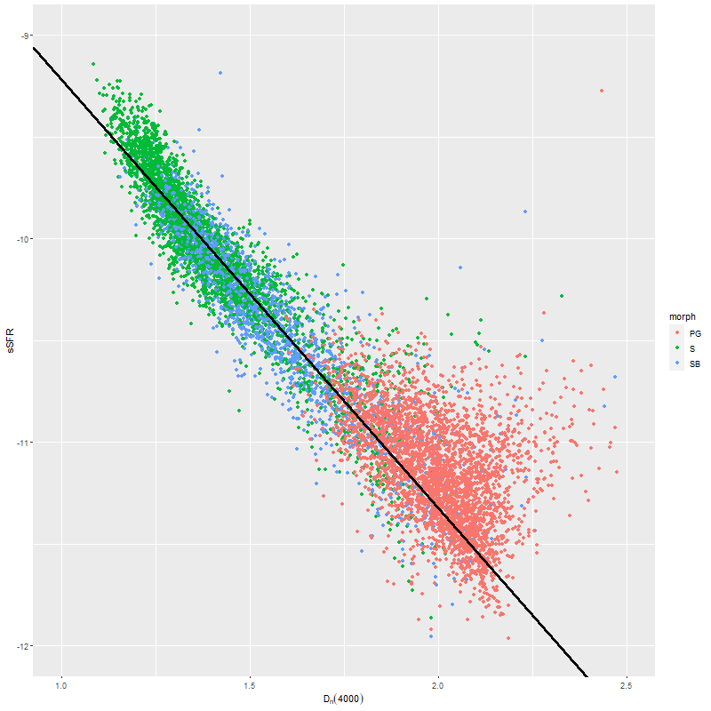
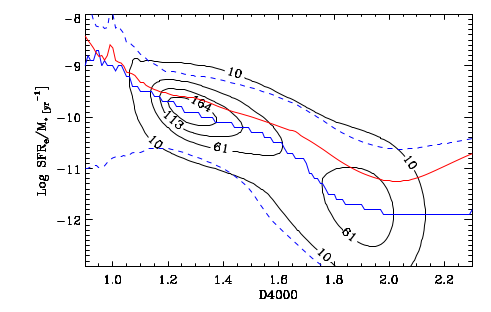
Second topic: the spectral region around the 4000Å “break” has long been known to be sensitive to stellar age. Its use as a quantitative specific star formation rate indicator apparently dates to Brinchmann et al. (2004)2They don’t cite any antecedents and I can’t find any either.. More recently Bluck et al. (2020) used a similar technique at the sub-galactic level on MaNGA galaxies. Both studies use D4000 as a secondary star formation rate indicator, preferring Hα luminosity as the primary SFR calibrator with D4000 reserved for galaxies (or regions) with non-starforming emission line ratios or lacking emission. Oddly, I have been unable to find an actual calibration formula in a slightly better than cursory search of the literature — both of the cited papers present schematic graphs with overlaid curves giving the adopted relationships and approximate uncertainties. The Brinchmann version from the published paper is copied and pasted below.
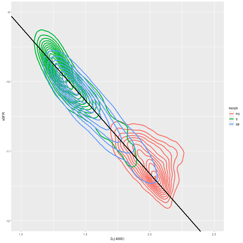
In the two graphs below I’ve added data from the passively evolving Coma cluster sample comprising 3348 binned spectra in 33 galaxies. There are two versions of the same graphs. Individual points are displayed in the first, as before with error bars suppressed to aid (slightly) clarity. The second displays the density of points at arbitrarily spaced contour intervals. The straight line is the “robust” regression line calculated for the spiral sample only, which for the sake of completeness is
\( \log10(sSFR) = -7.11 (\pm 0.02) – 2.11 (\pm 0.015) D_n(4000)\)
Model sSFR vs. measured value of D4000. 40 barred and non-barred spirals + 33 passively evolving Coma cluster galaxies.Model sSFR vs. measured value of D4000 (2D density version). 40 barred and non-barred spirals + 33 passively evolving Coma cluster galaxies.
Call:
lmrob(formula = ssfr_m ~ d4000_n, data = df.ssfr)
 \--> method = "MM"
Residuals:
       Min         1Q     Median         3Q        Max
-0.9802409 -0.0916555 -0.0005187  0.0962981  7.1748499

Coefficients:
            Estimate Std. Error t value Pr(>|t|)
(Intercept) -7.10757    0.02009  -353.8   <2e-16 ***
d4000_n     -2.10894    0.01418  -148.7   <2e-16 ***
---
Signif. codes:  0 ‘***’ 0.001 ‘**’ 0.01 ‘*’ 0.05 ‘.’ 0.1 ‘ ’ 1

Robust residual standard error: 0.1384
Multiple R-squared:  0.9043,	Adjusted R-squared:  0.9043
Convergence in 13 IRWLS iterations

Robustness weights:
 39 observations c(45,958,1003,1165,1200,1230,1249,1279,1280,1281,1282,1283,1294,1298,1299,1992,2040,2047,2713,2722,2723,2729,2735,2736,2974,3212,3226,3250,3667,3668,3671,3677,3685,3687,3688,3691,4056,4058,4083)
	 are outliers with |weight| <= 1.1e-05 ( < 2.1e-05);
 418 weights are ~= 1. The remaining 4310 ones are summarized as
     Min.   1st Qu.    Median      Mean   3rd Qu.      Max.
0.0001994 0.8684000 0.9514000 0.8911000 0.9850000 0.9990000
The relation between D4000 and sSFR as estimated by Brinchmann et al. 2004
All three groups follow the same relation but with some obvious differences in distribution. The non-barred spiral sample extends to higher star formation rates (either density or sSFR) than barred spirals, which in turn extend into the passively evolving range. The Coma cluster sample has a long tail of high D4000 values (or high specific star formation rates at given D4000) — this is likely because D4000 becomes sensitive to metallicity in older populations and this sample contains some of the most massive (and highest metallicity) galaxies in the local universe. Also, as I’ve noted before these models “want” to produce a smoothly varying mass growth history, which means that even the reddest and deadest elliptical will have some contribution from young populations. This seems to put a floor on modeled specific SFR of ∼10-11.5 yr-1.
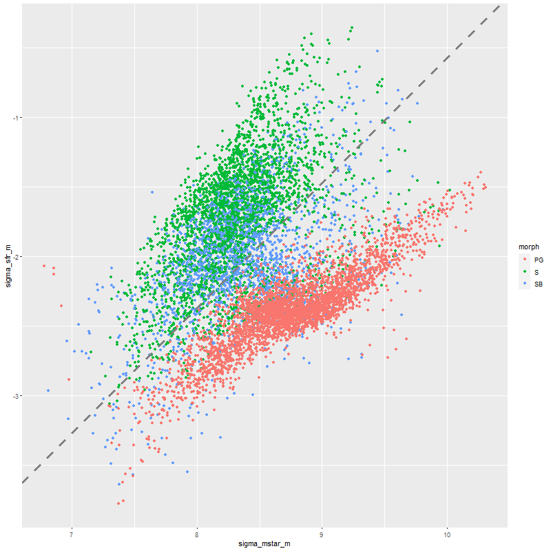
Just to touch briefly on the paper by Fraser-McKelvie et al. barred spirals in this sample do have lower overall star formation than non-barred, with large areas in the green valley or even passively evolving. This sample is too incomplete to say much more. For the sake of having a visualization here is the spatially resolved ΣSFR vs. ΣM* relation. The dashed line is Bluck’s estimate of the star forming “main sequence,” which looks displaced downward compared to my estimates.
Model SFR density vs. stellar mass density. 40 barred and non-barred spirals + 33 passively evolving Coma cluster galaxies.
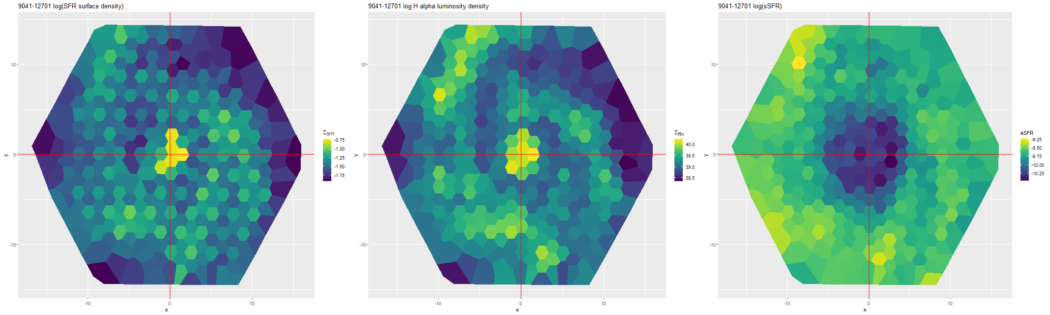
Finally, here are a couple of grand design spirals, one barred and one (maybe) not to illustrate how model results track morphological features. In the barred galaxy note that the arms are clearly visible in the SFR maps but they aren’t visible at all in the stellar mass map, which does show the presence of the very prominent bar.
NGC 6001 – thumbnail with MaNGA IFU footprintNGC 6001 (MaNGA plateifu 9041-12701)
(L) Model SFR surface density
(M) Hα luminosity density
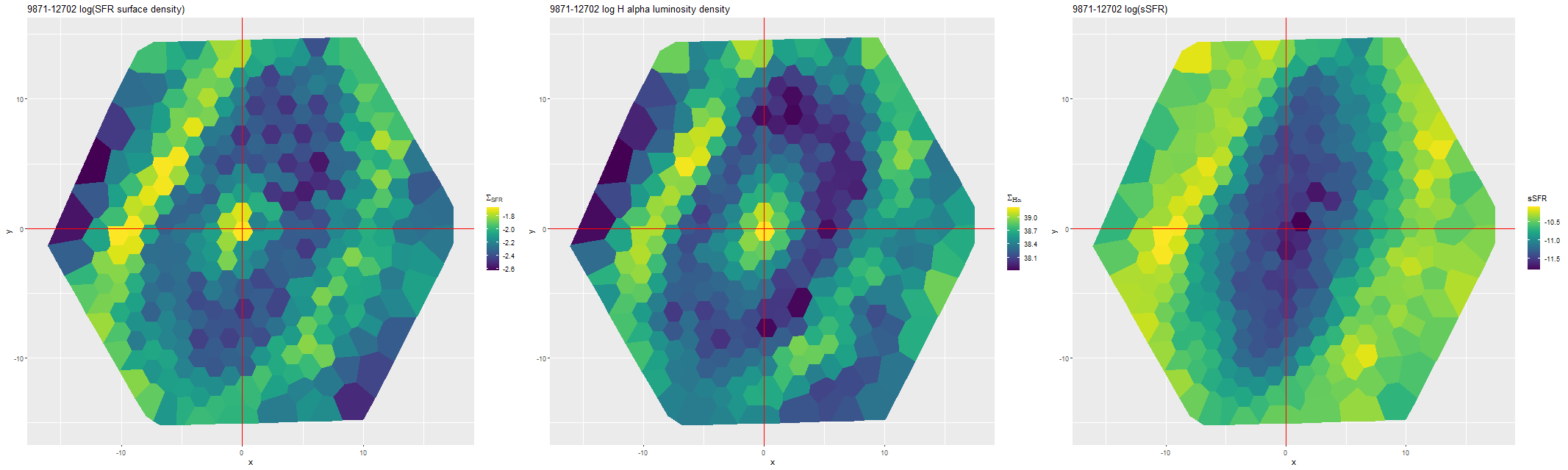
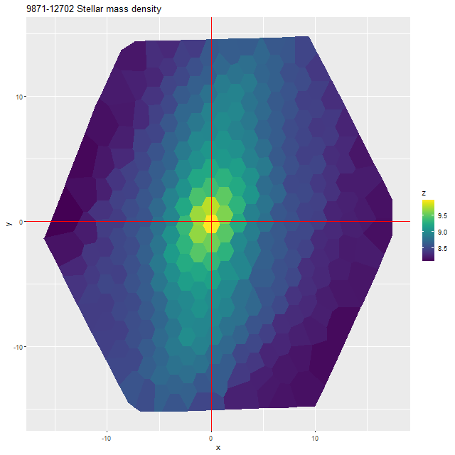
(R) sSFRNGC 5888- thumbnail with MaNGA IFU footprintNGC 5888 (MaNGA plateifu 9871-12702)
(L) Model SFR surface density
(M) Hα luminosity density
(R) sSFRNGC 5888 (MaNGA plateifu 9871-12702) – Log model stellar mass density (Msun/kpc2
I’m not sure how much more I’m going to do with normal spirals. As I’ve said repeatedly the full sample is much too large for my computing resources.
Next time (probably) I’m going to return to a very small sample of post-starburst galaxies, which I may also return to when the final SDSS public data is released.
I only have time to analyze one MaNGA galaxy for now and since it was the first to get the correctly coded LOSVD estimates I chose the Coma Cluster S0 galaxy NGC 4949 that I discussed in the last post for SFH modeling. As I mentioned a few posts ago trying to model the LOSVD and star formation history simultaneously is far too computationally intensive for my resources, so for now I just convolve the SSP model spectral templates with the elementwise means of the convolution kernels estimated as described previously and feed those to the SFH modeling code. My intuition is that the SFH estimates should be at least slightly more variable if the kinematics are treated as variable as well, but for now there’s no real alternative to just picking a fiducial value. Of course a limited test of that hypothesis could be made by pulling multiple draws from the posterior of the LOSVD distribution. I will certainly try that in the future.
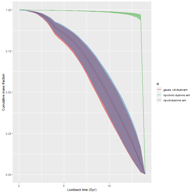
My first idea was to leave both dust and emission lines out of the SFH models. The first choice was to save CPU cycles and also based on the expectation that these passively evolving galaxies should have very little dust. The results were rather interesting: here are ribbon plots of model SFH’s for all 86 binned spectra. The pink ribbons are from the original model runs, which assumed single component gaussian velocity distributions, modified Calzetti attenuation, and included emission lines (which contribute negligible flux throughout). The blue ribbons are with non-parametric LOSVD and no attenuation model:
NGC 4949 – modeled star formation histories with single component gaussian and nonparametric estimates of line of sight velocity distributions with no dust model
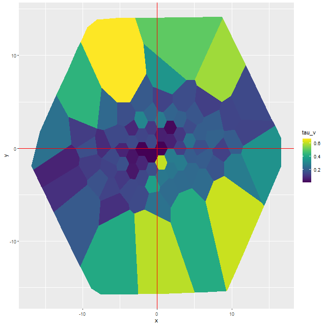
The differences in star formation histories turn out to be almost entirely due to neglecting dust in the second set of model runs. In this galaxy there are some areas with apparently non-negligible amounts of dust:
NGC 4949 – map of estimated optical depth of attenuation
Ignoring attenuation forces the model to use redder, hence older (and probably more metal rich although I haven’t yet checked) stellar populations and this has, in some cases, profound effects on the model SFH.
So, I tried a second set of model runs adding back in modified Calzetti attenuation but still leaving out emission:
NGC 4949 – modeled star formation histories with single component gaussian and nonparametric estimates of line of sight velocity distributions
And now the models are nearly identical, with minor differences mostly in the youngest age bin. All other quantities that I track are similarly nearly identical in both model runs.
Here is the modeled mass growth history for a single spectrum of a region just south of the nucleus that had the largest difference in model SFH in the second set of runs, and the largest optical depth of attenuation in the first and 3rd. This is an extreme case of the shift towards older populations required by the neglect of reddening. Well over 90% of the present day stellar mass was, according to the model, formed in the first half Gyr after the big bang with almost immediate and complete quenching thereafter. While not an impossible star formation history it’s not one I often see result from these models, which strongly favor more gradual mass buildup.
NGC 4949 – modeled mass growth histories for models with and without an attenuation model
So, the conclusion for now is that having an attenuation model matters a lot, the detailed stellar kinematics not so much. Of course this is a relatively simple example because it’s a rapid rotator and the model convolution kernels are fairly symmetrical throughout the galaxy. The massive ellipticals and especially cD galaxies with more complex kinematics might provide some surprises.
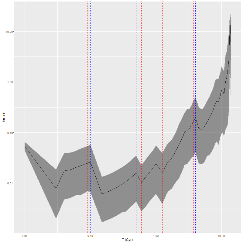
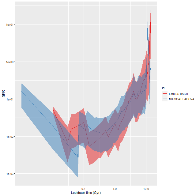
One of my favorite visualization tools for displaying results of star formation history modeling is a ribbon plot of star formation rate versus look back time. This simply plots the marginal posterior mean or median SFR along with 2.5 and 97.5th percentiles (by default) as the lower and upper boundaries of the ribbon. I’ve been using the simplest possible definition of the star formation rate, namely the total mass born in each age bin divided by the interval between the nominal age of each SSP model and the next younger. One striking feature of these plots that’s especially evident in grids of SFH models for an entire galaxy like the one shown in my last post is that there are invariably jumps in the SFR at certain specific ages as marked below. This particular example is from a sample of passively evolving Coma cluster galaxies, but the same features are seen regardless of the likely “true” star formation history.
Star formation rate history estimate – emiles with BaSTI isochrones
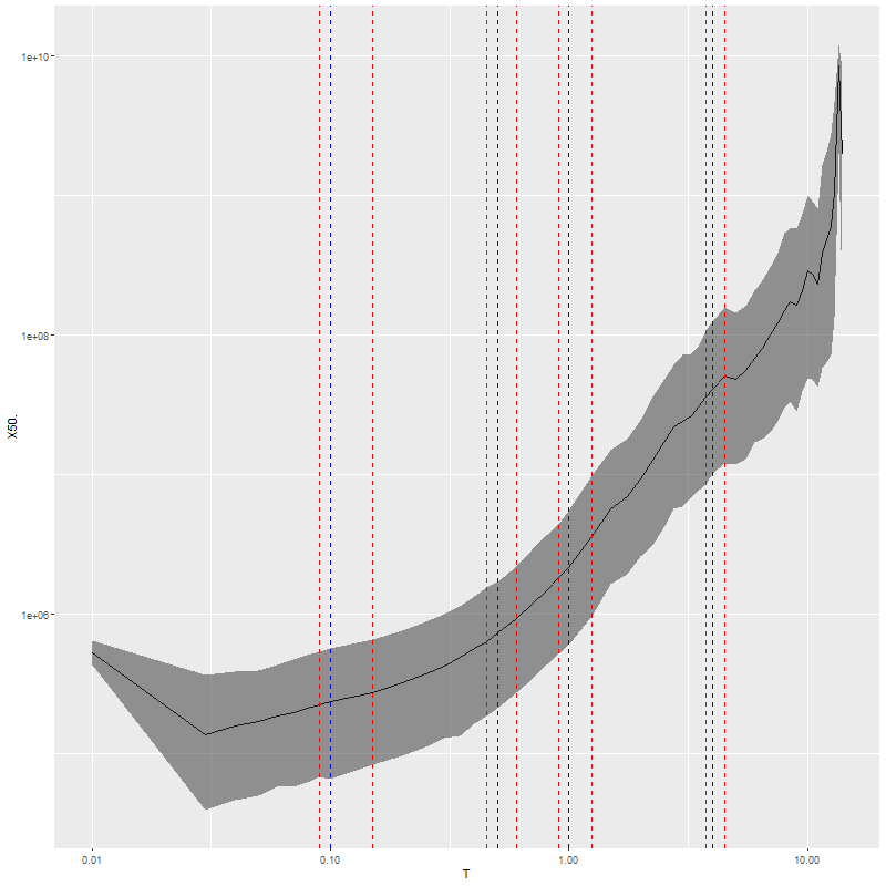
These jumps are artifacts of course: the BaSTI isochrones used for the EMILES SSP models that I currently use are tabulated at age intervals that are constant over certain age ranges, with jumps at 4 ages1100 Myr, 500 Myr, 1 Gyr, and 4 Gyr. The jumps in model SFR occur exactly at the breaks in the age intervals. This turns out to be due to an otherwise welcome feature of the SFH models that they “want” to produce SSP contributions that vary smoothly with age as shown below for the same model run. So for example the stellar mass born in the 90-100 Myr age bin per the model is about 90% of that in the 100-150 Myr bin while the time interval increases by a factor of 5, so the model SFR declines by a factor 4.5 or around 0.6 dex.
Modeled mass born in each age bin – central spectrum of plateifu 9876-12702
Can I do anything about this? Should I? Changing how I calculate the star formation rate might work — this is after all a derivative and I’m currently using the most stupidly simple numerical approximation possible. It also might help to adjust the effective ages of each SSP model. I should also look at the priors on the SSP model coefficients, although as I noted some time ago it’s hard to affect the model star formation histories much with adjustments to priors.
These jumps are something of a peculiarity of the BaSTI isochrones. I had previously used a subset of MILES SSP models from Padova isochrones, which are tabulated at equal logarithmic age intervals. A comparison model run lacks large jumps except for an early time burst. Since the youngest age bin in the Padova isochrones is around 60 Myr I had added two younger SSP models from an update of the BC03 library, and these show abrupt jumps in model SFR. This is also the case with the youngest age bin in my currently used EMILES library.
Comparison of star formation rate history estimates:
Red – EMILES SSP libraries with BaSTI isochrones
Blue – Miuscat SSP library with Padova isochrones
A final comment about these visualizations is that often the mode of the posterior distribution of an SSP model contribution is near 0, and it might make sense to display one sided confidence intervals since what we’re really constraining is an upper limit. I may work on this in the future.
It took a few months but I did manage to analyze 28 of the 29 galaxies in the sample I introduced last time. One member — mangaid 1-604907 — hosts a broad line AGN and has broad emission lines throughout. That’s not favorable for my modeling methods, so I left it out. It took a while to develop a more or less standardized analysis protocol, so there may be some variation in S/N cuts in binning the spectra and in details of model runs in Stan. Most runs used 250 warmup and 750 total iterations for each of 4 chains run in parallel, with some adaptation parameters changed from their default values1I set target acceptance probability adapt_delta to 0.925 or 0.95 and the maximum treedepth for the No U-Turn Sampler max_treedepth to 11-12. A total post-warmup sample size of 2000 is enough for the inferences I want to make. One of the major advantages of the NUTS sampler is that once it converges it tends to produce draws from the posterior with very low autocorrelation, so effective sample sizes tend to be close to the number of samples.
I’m just going to look at a few measured properties of the sample in this post. In future ones I may look in more detail at some individual galaxies or the sample as a whole. Without a control sample it’s hard to say if this one is significantly different from a randomly chosen sample of galaxies, and I’m not going to try. In the plots shown below each point represents measurements on a single binned spectrum. The number of binned spectra per galaxy ranged from 15 to 153 with a median of 51.5, so a relatively small number of galaxies contribute disproportionately to these plots.
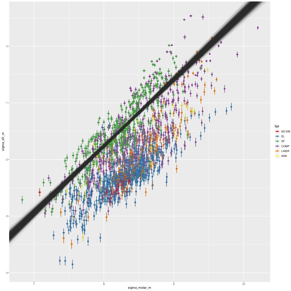
One of the more important empirical results in extragalactic astrophysics is the existence of a fairly well defined and approximately linear relationship between stellar mass and star formation rate for star forming galaxies, which has come to be known as the “star forming main sequence.” Thanks to CALIFA and MaNGA it’s been established in recent years that the SFMS extends to subgalactic scales as well, at least down to the ∼kpc resolution of these surveys. This first plot is of the star formation rate surface density vs. stellar mass surface density, where recall my estimate of SFR is for a time scale of 100 Myr. Units are \(\mathrm{M_\odot /yr/kpc^2} \) and \(\mathrm{M_\odot /kpc^2} \), logarithmically scaled. These estimates are uncorrected for inclination and are color coded by BPT class using Kauffmann’s classification scheme for [N II] 6584, with two additional classes for spectra with weak or no emission lines.
If we take spectra with star forming line ratios as comprising the SFMS there is a fairly tight relation: the cloud of lines are estimates from a Bayesian simple linear regression with measurement error model fit to the points with star forming BPT classification only (N = 428). The modeled relationship is \(\Sigma_{sfr} = -11.2 (\pm 0.5) + 1.18 (\pm 0.06)~ \Sigma_{M^*}\) (95% marginal confidence limits), with a scatter around the mean relation of ≈ 0.27 dex. The slope here is rather steeper than most estimates2For example in a large compilation by Speagle et al. (2014) none of the estimates exceeded a slope of 1., but perhaps coincidentally is very close to an estimate for a small sample of MaNGA starforming galaxies in Lin et al. (2019). I don’t assign any particular significance to this result. The slope of the SFMS is highly sensitive to the fitting method used, the SFR and stellar mass calibrators, and selection effects. Also, the slope and intercept estimates are highly correlated for both Bayesian and frequentist fitting methods.
One notable feature of this plot is the rather clear stratification by BPT class, with regions having AGN/LINER line ratios and weak emission line regions offset downwards by ~1 dex. Interestingly, regions with “composite” line ratios straddle both sides of the main sequence, with some of the largest outliers on the high side. This is mostly due to the presence of Markarian 848 in the sample, which we saw in recent posts has composite line ratios in most of the area of the IFU footprint and high star formation rates near the northern nucleus (with even more hidden by dust).
Σsfr vs. ΣM*. Cloud of straight lines is an estimate of the star-forming main sequence relation based on spectra with star-forming line ratios. Sample is all analyzed spectra from the set of “transitional” candidates of the previous post.
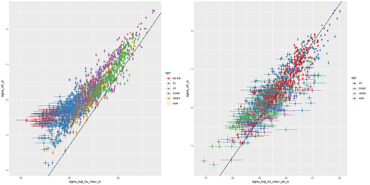
Another notable relationship that I’ve shown previously for a few individual galaxies is between the star formation rate estimated from the SFH models and Hα luminosity, which is the main SFR calibrator in optical spectra. In the left hand plot below Hα is corrected for the estimated attenuation for the stellar component in the SFH models. The straight line is the SFR-Hα calibration of Moustakas et al. (2006), which can be traced back to early ’90s work by Kennicutt.
Most of the sample does follow a linear relationship between SFR density and Hα luminosity density with an offset from the Kennicutt-Moustakas calibration, but there appears to be a departure from linearity at the low SFR end in the sense that the 100 Myr averaged SFR exceeds the amount predicted by Hα (which recall traces star formation on 5-10 Myr scales). This might be interpreted as indicating that the sample includes a significant number of regions that have been very recently quenched (that is within the past 10-100 Myr). There are other possible interpretation though, including biased estimates of Hα luminosity when emission lines are weak.
In the right hand panel below I plot the same relationship but with Hα corrected for attenuation using the Balmer decrement for spectra with firm detections in the four lines that go into the [N II]/Hα vs. [O III]/Hβ BPT classification, and therefore have firm detections in Hβ. The sample now nicely straddles the calibration line over the ∼ 4 orders of magnitude of SFR density estimates. So, the attenuation in the regions where emission lines arise is systematically higher than the estimated attenuation of stellar light. This is a well known result. What’s encouraging is it implies my model attenuation estimates actually contain useful information.
(L) Estimated Σsfr vs. Σlog L(Hα) corrected for attenuation using stellar attenuation estimate.
(R) same but Hα luminosity corrected using Balmer decrement. Spectra with detected Hβ emission only.
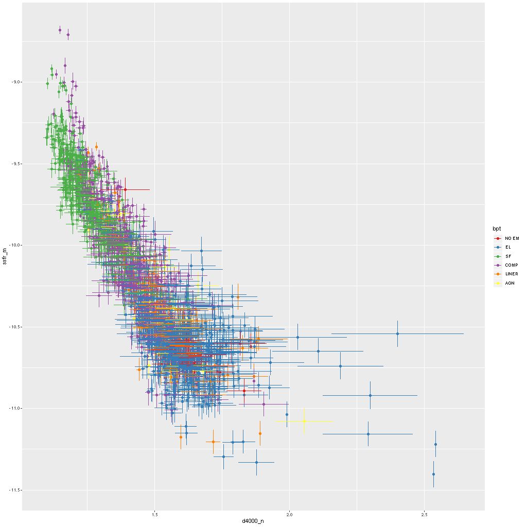
One final relation: some measure of the 4000Å break strength has been used as a calibrator of specific star formation rate since at least Brinchmann et al. (2004). Below is my version using the “narrow” definition of D4000. I haven’t attempted a quantitative comparison with any other work, but clearly there’s a well defined relationship. Maybe worth noting is that “red and dead” ETGs typically have \(\mathrm{D_n(4000)} \gtrsim 1.75\) (see my previous post for example). Very few of the spectra in this sample fall in that region, and most are low S/N spectra in the outskirts of a few of the galaxies.
Specific star formation rate vs. Dn4000
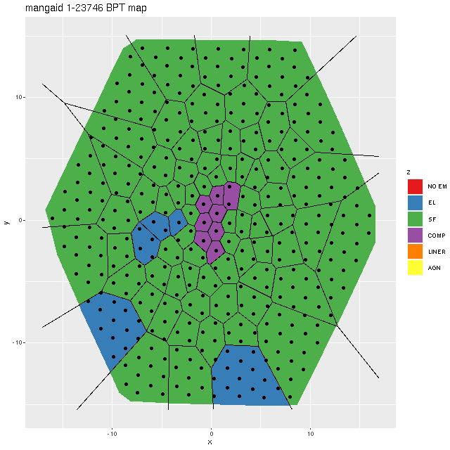
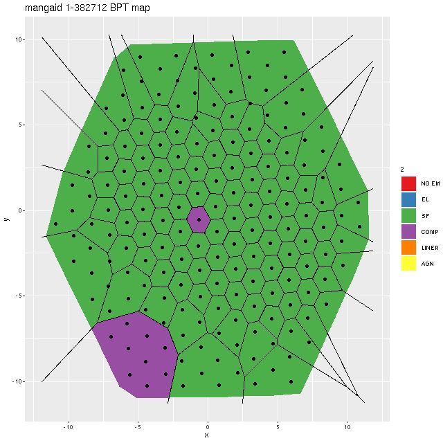
Two obvious false positives in this sample were a pair of grand design spirals (mangaids 1-23746 and 1.382712) with H II regions sprinkled along the full length of their arms. To see why they were selected and verify that they’re in fact false positives here are BPT maps:
Map of BPT classification — mangaid 1-23746 (plateifu 8611-12702)Map of BPT classification — mangaid 1-382712 (plateifu 9491-6101)
These are perfect illustrations of the perils of using single fiber spectra for sample selection when global galaxy properties are of interest. The central regions of both galaxies have “composite” spectra, which might actually indicate that the emission is from a combination of AGN and star forming regions, but outside the nuclear regions star forming line ratios prevail throughout.
These two galaxies contribute about 45% of the binned spectra with star forming line ratios, so the SFMS would be much more sparsely populated without their contribution. Only one other galaxy (mangaid 1-523050) is similarly dominated by SF regions and it has significantly disturbed morphology.
I may return to this sample or individual members in the future. Probably my next posts will be about Bayesian modelling though.