This will be short. I’ve provisionally decided to proceed with the Progeny based SSP model libraries I’ve discussed over the last several posts. I’ve picked two versions for model runs: a “small” one with 5 metallicity bins and 42 age bins from log(T) = 6 to 10.1 in 0.1 dex intervals, and a “medium” sized one with just 3 metallicities (log(Z/Z☉) = {-0.25, 0, +0.5}) and 74 age bins with log(T) = 6.0, 6.5 and 6.55, … , 10.1 in 0.05 dex intervals. These all use the MIST isochrones, Kroupa IMF, and the recommended stellar ingredients from the first Progeny paper. As discussed in a previous post the wavelength interval is limited to 3300 – 9000Å because of the prevalence of terrestrial night sky lines and calibration issues in the near IR portion of MaNGA spectra.
I’ve decided to take one more, maybe final, look at a sample of SDSS selected galaxies in MaNGA. I remembered recently that I’ve made several attempts to select post-starburst samples with various queries of SDSS databases. One I did some time ago had nearly 5800 hits in DR8, with 104 cross matches in MaNGA. Part of the query is pasted below:
select into mydb.mylargerka
  s.ra,
  s.dec,
  s.plate,
  s.mjd,
  s.fiberid,
  s.z,
  s.zErr,
  from specObj s
  left outer join galSpecline as g on s.specObjid = g.specObjid
  left outer join galSpecIndx as gi on s.specObjid = gi.specObjid
  left outer join galSpecExtra as ge on s.specObjid = ge.specObjid
where
  (g.oii_3729_eqw > -5 and g.oii_3729_eqw_err > 0) and
  (gi.lick_hd_a_sub > 4 and gi.lick_hd_a_sub_err > 0) and
  s.z >= .02 and
  (s.snMedian > 10) and
  (s.zWarning = 0 or s.zWarning = 16)
  order by
  s.plate, s.mjd, s.fiberid
So basically this is just a standard sort of post-starburst selection with relaxed limits on both Balmer absorption and emission line strength. The line index data were from the MPA/JHU pipeline, which was last run on DR8.
I had run models for about 1/4 of the 104 galaxy sample when a heat wave arrived, and I decided for the sake of our electric bills not to continue intensive computing 24/7. Temperatures are currently below normal, so I may be able to resume soon. About all I can say so far is the sample contains a mix of known PSBs and false positives — which are mostly ordinary star forming galaxies.
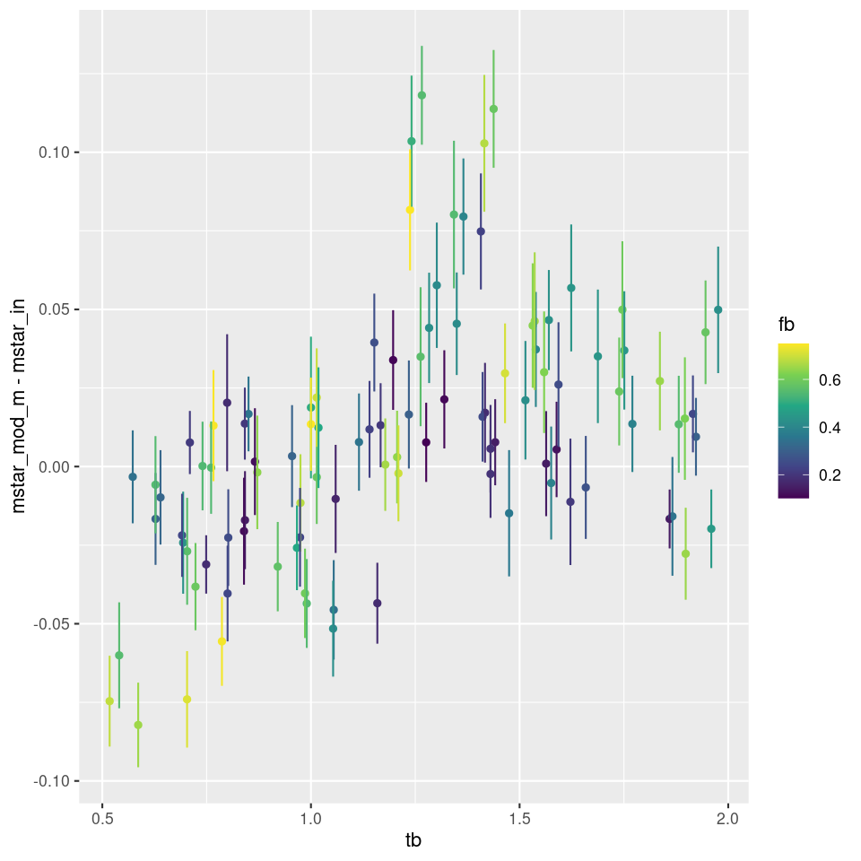
A few brief comments about the simulations, of which I’ve done a few more but will probably bring to an end. First, here is a plot I mentioned but didn’t display last time of the bias in stellar mass estimate against the lookback time to the burst. Points are color coded by burst strength.
Bias is stellar mass estimate vs. lookback time to burst (simulations)
There appears to be a weak trend with burst age up to about 1 Gyr, but at all burst ages and strengths there are biases on both sides of zero. It isn’t clear to me what, if anything else, is driving biases in either direction. The one thing I can say for sure is that the models are overconfident in their ability to estimate the stellar mass since the typical 1σ error bar is under 0.02 dex while the scatter is around ±0.1 dex. I actually think 25% uncertainty in stellar mass estimates is optimistic.
I remembered a short while ago that “outshining” is the term of art in the industry for the situation in which light from recent star formation overwhelms that of the older population. This seems to be a fairly major concern in the literature. A full text search of ADS found 722 instances of its use in the astronomical literature with an explosion of usage after 2006. A quick scan of titles suggests perhaps half of the papers are about SFH modeling. Of course the word is often used in other contexts.
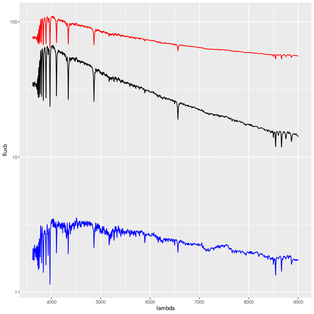
As a slightly more stringent test for outshining I ran one more simulation with a more recent and stronger starburst (tb=0.25 Gyr, fb = 1) than the earlier simulations. Even though the light of the burst population dominates the old base population the latter does have some effect of the combined spectrum (in red below, and offset vertically for clarity): it is redder and the line strengths are altered somewhat relative to the burst population.
Synthetic spectra – strong recent starburst. Fluxes are logarithmically scaled. Total flux (red) is vertically offset.
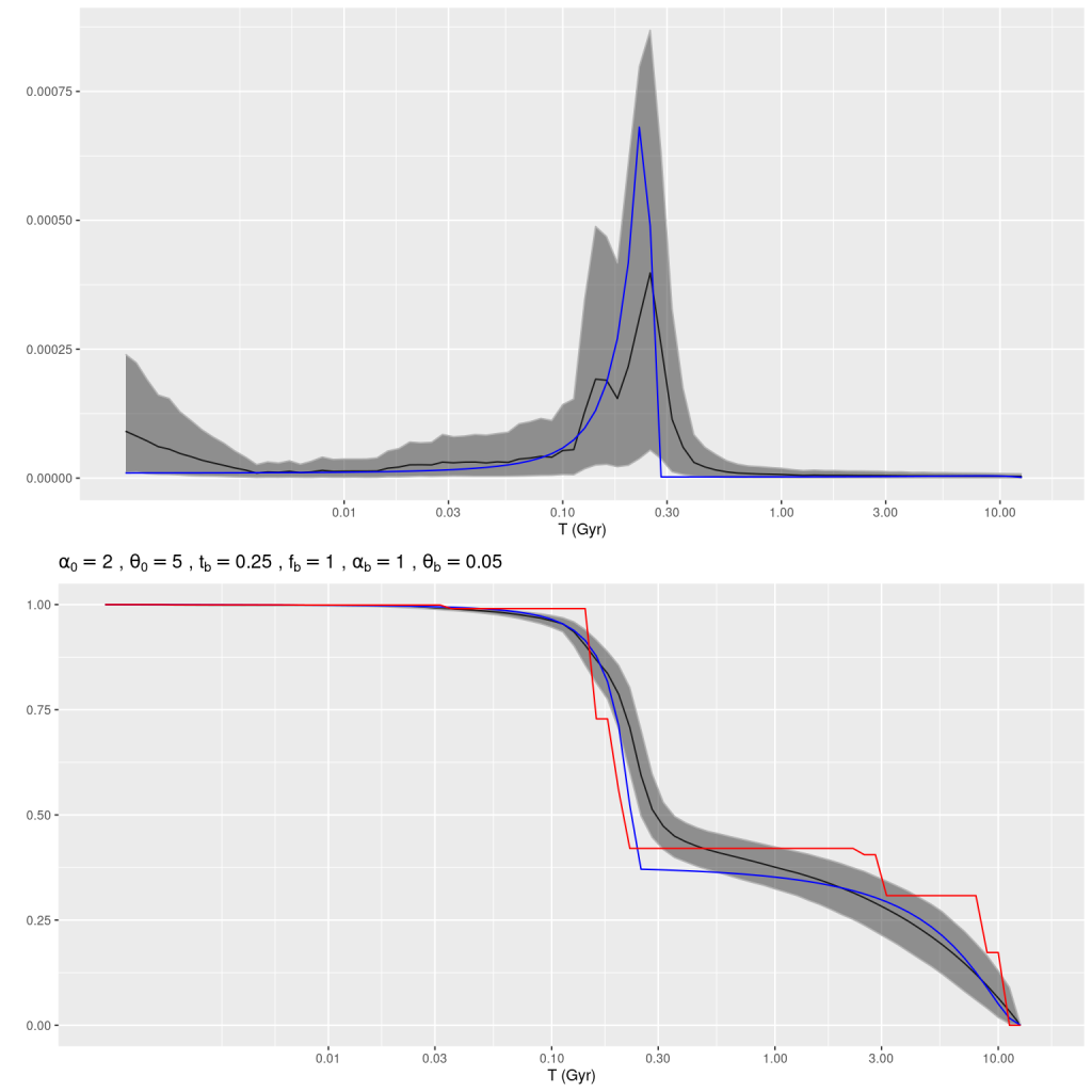
The model actually captures both the ancient and recent star formation history rather well. The mass growth marginal confidence band at old ages covers the input right up to the beginning of the burst build up, and the post-burst SFR is modeled accurately. The total mass in the model slightly exceeds the input: log(M*) = 4.88±0.02 model, 4.84 input. The model specific star formation rate is nearly identical: -9.33±0.08 model, -9.36 input.
Simulation – strong recent starburst
Shortly after starting these simulations I noticed a paper by Suess et al. (2022) describing simulations with a similar objective of testing the ability of a code named PROSPECTOR to recover star formation histories of post-starburst galaxies in the ideal case of inputs matched to the model, i.e. the inputs are used to generate the mock data and then to fit it. I’m not going to say a lot about either the code or paper. IIRC the first published description of the code (Leja et al. 2017) claimed it to be the first to model non-parametric star formation histories in a fully Bayesian framework. As far as I know this is true in the published literature but they only could use a few very broad time bins; the version used in Suess uses 9. I was already using the full time resolution of my adopted SSP model libraries by then.
The 2022 paper only shows a single, no doubt cherry picked example of a fit to mock data. Like mine their model star formation histories fail to cover the inputs for some age ranges. On the other hand their fits to a mock spectrum appear to be rather poor with large systematic errors. In every model run of mine residuals look very much like 0 mean Gaussian white noise with the expected deviance. They appear to show a similar range of deviations from input stellar masses with no significant error in the mean. Another striking similarity is they find a definite floor to late time star formation rates. As I’ve noted many times my models will always include some contribution from very young populations and there seems to be a floor around 10-11.5 /yr in specific star formation rate.
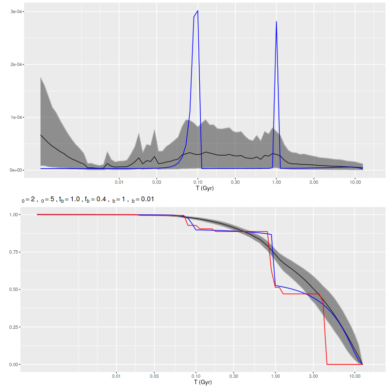
A much more recent paper by the same group (Wang et al. 2025) looked at simulated data from quite different systems, namely ones with bursty star formation on short time scales. Their work was motivated by yet more simulations of galaxy formation in the early universe. I’m again not going to comment much on this paper except to notice that they concluded that “given the correct SFH model, it is indeed possible to infer the SFH by performing SED fitting.” In other words they had to fine tune their prior to get to the right posterior. I’m sure it’s not as tautological as that sentence appears. Anyway, this motivated me to take a brief look at a few multiple burst simulations. The one shown below has two very sharply peaked ones with roughly the same peak SFR but more total mass in the older one. The model has spread out star formation over the entire interval between the input bursts with a slower rise and decay. Once again the maximum likelihood fit obtained with non-negative least squares captures the timing and relative magnitude of the bursts rather well.
Simulation – 2 short starbursts
Recall that my stellar contribution estimates are parametrized as an N-simplex with an implicit Dirichlet prior with concentration parameter α = 1, which is uniform on the simplex. In principle adopting an explicit prior with a concentration parameter < 1 should encourage a more bursty star formation history without favoring any particular ages, and it did (this run used α = 0.25):
Simulation – 2 short starbursts, modified prior
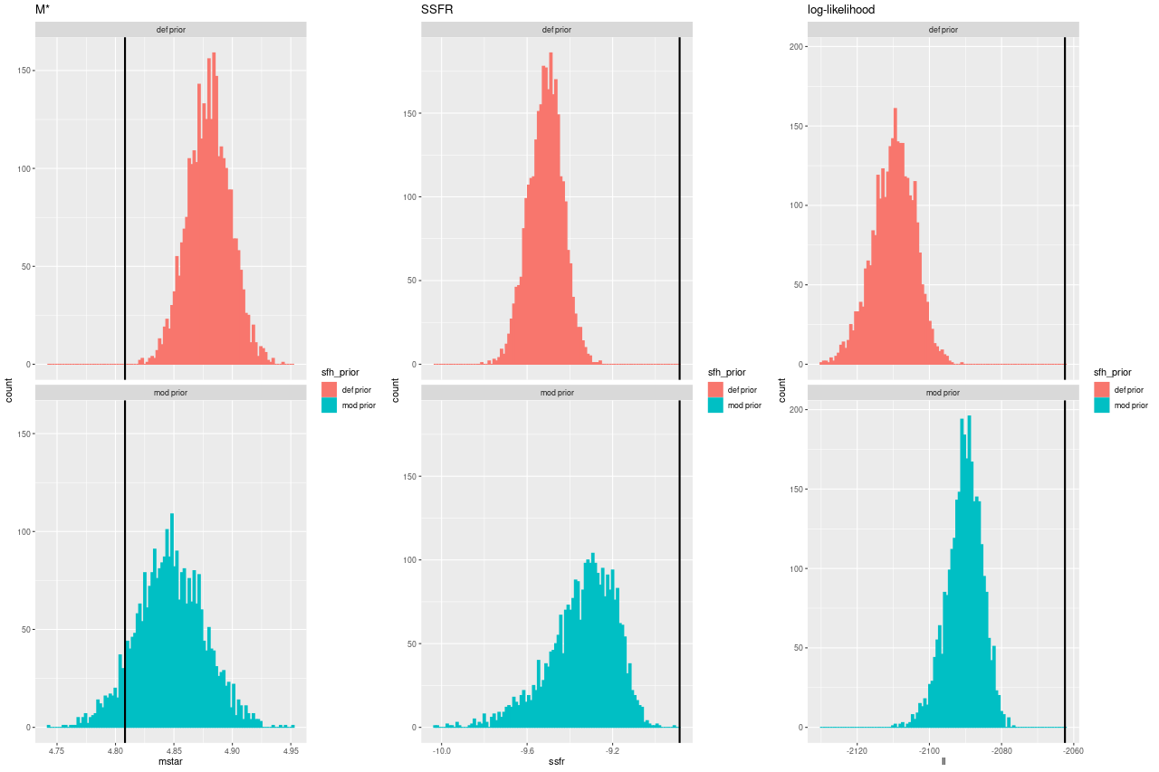
Here are histograms of a few summary quantities I track: the present day stellar mass, specific star formation rate (100 Myr average), and the summed log-likelihood of the fits to the spectra. Both runs underestimated the sSSFR because the recent burst was more spread out in the models.
Two burst simulation: comparing two priors on stellar contributions for sampled stellar mass, SSFR, and log-likelihood of fits
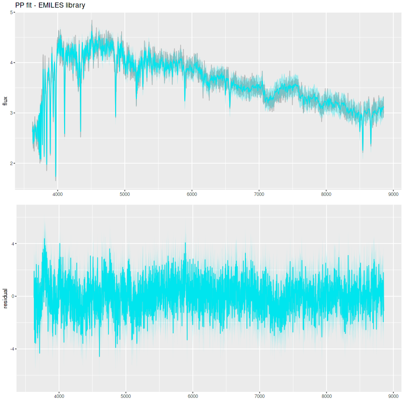
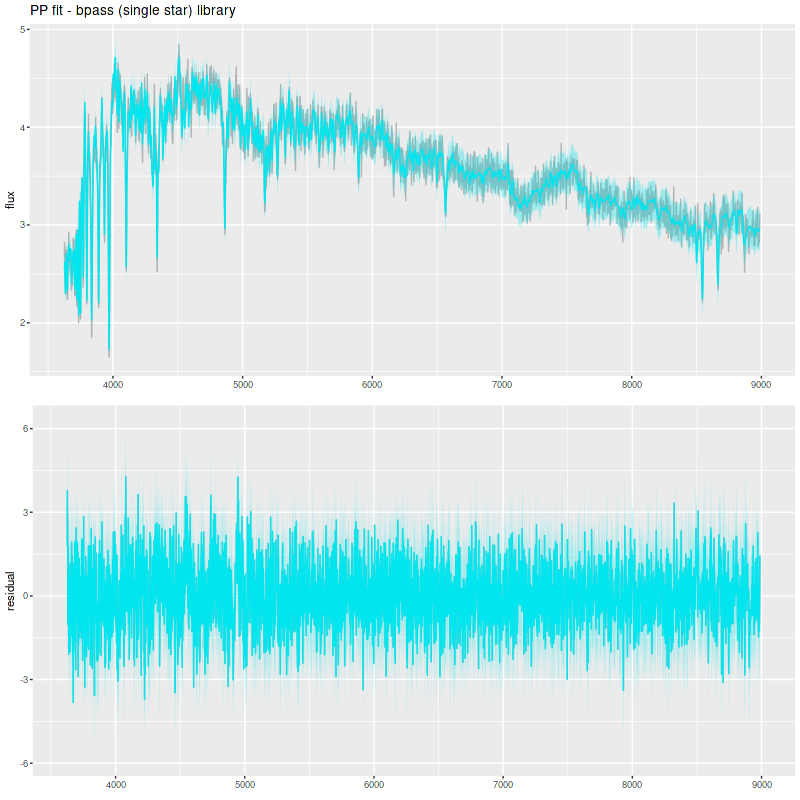
Finally, I did a few runs with two other libraries: EMILES, which has been my base SSP model library for some time, and BPASS with single star evolution and an upper mass limit of 100 M☉. The parameters I used for the star formation history resulted in a gentle late time revival rather than a burst. Both model runs had late time bursts, although the mass added was negligible. The EMILES run has the characteristic jumps at ages where the age intervals change. Although it’s small the BPASS run has the jump at 1.6 Gyr that I noted previously.
Simulation with C3K input and EMILES as test library
As with real data the EMILES models have some systematic errors around the trough around 7000-7300Å, and also in the blue near the Balmer break.
The BPASS models fit the data surprisingly well, despite using completely different sources for stellar atmospheres.
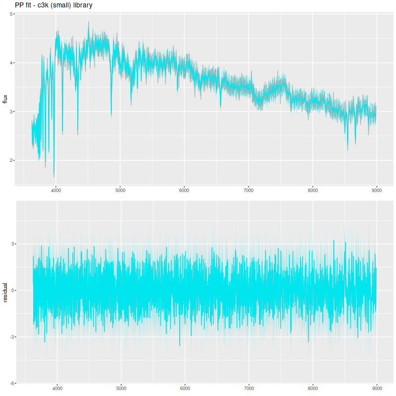
Comparison PP fit with C3K as test library:
The table below summarizes a couple of the quantities I track. The Progeny C3K models that were used to create the inputs recovers them flawlessly. The other two recover the mass (BPASS is low by more than its nominal uncertainty), but are biased on the high side in late time star formation rate estimates.
Stellar mass
sSFR
input
4.78
-9.91
Progeny C3K
4.78 (0.017)
-9.90 (0.054)
EMILES
4.82 (0.012)
-9.62 (0.028)
BPASS
4.67 (0.03)
-9.73 (0.049)
I’m going to get back to real data now using the Progeny generated libraries. The simulations were a useful exercise if for no other reason than to show that timing faded starbursts can’t be done very accurately, at least with full spectrum fitting at visual wavelengths. I did get some ideas for small code improvements, and the idea of stacking star formation rate and mass growth histories seems like a useful visualization tool.
I’ve decided to take a break from real galaxy data and run some simulations of synthetic galaxy spectra. The main motivation was to help make an informed decision about which subset of the ProGeny based SSP libraries to use: the ones based on the MIST isochrones have ages uniformly logarithmically spaced at 0.05 dex intervals and 15 metallicity bins. Most of the latter are considerably sub-solar and aren’t likely to be major contributors to the light of nearby massive galaxies. For possibly metal poor dwarf galaxies it’s always possible to pick a metal poor subset — I have a subset of EMILES that I’ve used for that purpose for some time. More important to me is the choice of age bins. As I mentioned in the last post I did model runs with both 42 (0.1 dex age intervals) and 83 ages, with SSP models younger than log(T) = 6 and older than the currently accepted age of the universe excluded. Since execution time of a Stan model is roughly proportional to the number of parameters and these models are rather time consuming I’d like to know if the coarser age spacing has sufficient resolution. I will show below why it’s correct to exclude the very youngest populations.
Other reasons to do these kinds of exercises are to test the accuracy of retrieval of key quantities in idealized conditions where model assumptions are met by the inputs, to compare different model libraries, or to compare different modeling codes (something I don’t plan to do at present). Performing simulations is de rigueur in the SFH modeling industry and there are many examples in the literature, both as appendices and standalone papers — to name one the second of the two ProGeny papers I linked last time falls in this category. I’ve even done some limited simulations as far back as 2018, but the only case I wrote about was a very simple one.
This time I’ve decided to be more systematic and at least slightly more realistic. Since I remain interested in post-starburst galaxies I am creating simulations with two components: a base population that begins forming stars at the beginning of the universe, which I take to be a lookback time of \(10^{10.125}\) yr. = \(13.36\) Gyr. The second component is a “burst” population that commences star formation at a lookback time of \(\mathsf{t}_b\) with a relative strength of \(\mathsf{f}_b\). The base population has solar metallicity (Z = 0.02) while the burst is slightly subsolar (log(Z/Z☉) = -0.25). This obviously isn’t meant to represent a realistic model for chemical evolution — the purpose again is to test the ability to recover the input stellar metallicities in idealized circumstances. In keeping with my usual attitude of treating this as an afterthought I haven’t gotten around to exploring this issue yet.
Both the base and burst populations have time varying star formation rates proportional to Gamma probability distributions. The Gamma distribution is a two parameter family of univariate functions that can have a fairly wide variety of shapes, all of which have a single mode at \(t \ge 0\) followed by a monotonic decline asymptotically approaching 0. See the table below for the most salient properties. I don’t know of any real astrophysical justification1Abramson et al. (2016) argued for a log-normal form for the evolution of the cosmic SFR density and suggested that this describes the evolution of individual galaxies as well. More recently Katsianis, Yang, and Zheng (2021) argued for a gamma distribution fit to the evolution of the CSFRD and again claimed with some physical motivation that this form holds for individual galaxies. I was unaware of the latter work when I started this exercise. for this choice but it’s notable that it includes two of the most popular parametric forms for modeling star formation histories: exponentially declining (\(\alpha = 1\)), and what’s generally called the “delayed-\(\tau\)” model (\(\alpha =2\)) in the literature. Note that using a probability distribution has nothing to do with probability per se, but a probability density has two useful properties: it’s non-negative on its support and has a finite integral (equal to one when properly normalized).
Given shape and scale parameters the mass in each time bin is proportional to the difference in the cumulative gamma distribution at the beginning and end of each interval. The star formation history for each component is just the mass formed in all age bins, with the burst component multiplied by the burst strength. These are scaled to sum to 1, and the spectra are straightforwardly calculated as matrix products of the input SSP model fluxes with the mass histories. The “flux” values are multiplied by 105 for the sole purpose of making them approximately unit scaled. This has the effect of making the total mass born in the simulated “galaxy” equal to 105 M☉. The fluxes are interpolated to the same logarithmic wavelength grid used by SDSS, convolved with a gaussian to simulate stellar velocity dispersion, then truncated to the wavelength range (3621 Å, 9000 Å). The velocity dispersion is a settable parameter, but so far I have only used 140 km/sec. The base and burst spectra, which were calculated separately for visualization purposes are added, then multiplied by Calzetti attenuation with a user selected optical depth, then finally perturbed with Gaussian random noise. The flux variances are Poisson-like, that is they are proportional to the “counts” in each wavelength bin and scaled to a target average signal to noise. Again this is a settable parameter, but so far I have used a target SNR of 40, which is fairly typical for a fiber spectrum near the center of the IFU of a bright MaNGA galaxy. So far at least I do not add emission lines, but they are allowed in the models.
The subsequent modeling workflow is essentially the same as I use with real data, with some very minor tweaks reflecting the fact that the flux values are arbitrarily scaled. The Stan code is exactly the same as my current working version. Model runs use the same number of warmup and sampling iterations as my real data runs (250 and 750 respectively with 4 independent chains). Post processing is also essentially the same. I extract the posterior predictive fits to the spectra, the model star formation histories, the optical depth of attenuation and the reddening curve slope parameter. I compute the present day stellar mass, the 100 Myr averaged star formation rates, and specific SFR. The stellar mass and SFR are arbitrarily scaled but would scale by the same factor if these were real data from a distant galaxy, so the SSFR would be the same.I also track a few observables: the 4000 Å break index Dn(4000) and HδA.
This time I am exploring a wider range of star formation histories than my previous effort, which only examined a case or two with instantaneous bursts. With seven parameters (plus two more that I’ve held constant so far) it isn’t really practical to do a comprehensive grid of models, so for the most part I have randomly selected parameter values in the ranges shown below. At the time of writing I’ve run a few more than a hundred models. Most of these use the “small” version of the ProGeny C3K base SSP models as the test library, with a few using the input library as the test. I’ve also done a few with the “large” version (see the previous post for details of the ingredients). I plan to do some simulations with the other model libraries I’ve used, especially EMILES, but that’s somewhat of a different project. For now I’m examining the accuracy of outputs for the idealized case where the inputs satisfy the assumptions of the model.
\( \alpha_0 \in [1, 2] \)
\(\theta_0 \in [2, 6] \)
\(\mathsf{t}_b \in [0.5, 2]\)
\(\mathsf{f}_b \in [0.1, 0.75]\)
\( \alpha_b \in [1, 2] \)
\( \theta_b \in [0.01, 0.25] \)
\( \tau_V \in [0.0, 0.5] \)
Here is a cherry-picked example of a fairly strong and recent burst, using the small C3K based library as the test. First is the “observed” spectrum and the replicated values from the posterior (top pane), and the posterior residuals (bottom pane). The residuals look very much like — and pass standard statistical tests for — Gaussian white noise. This is rather different than I usually see with real data, of which a number of examples can be found by scrolling down through previous posts, where there are often large regions of spectra that are systematically misfit. This reflects the fact that all model assumptions are met by the data by construction, so fitting the data is expected.
Simulated spectrum and “posterior predictive” fit and residuals.
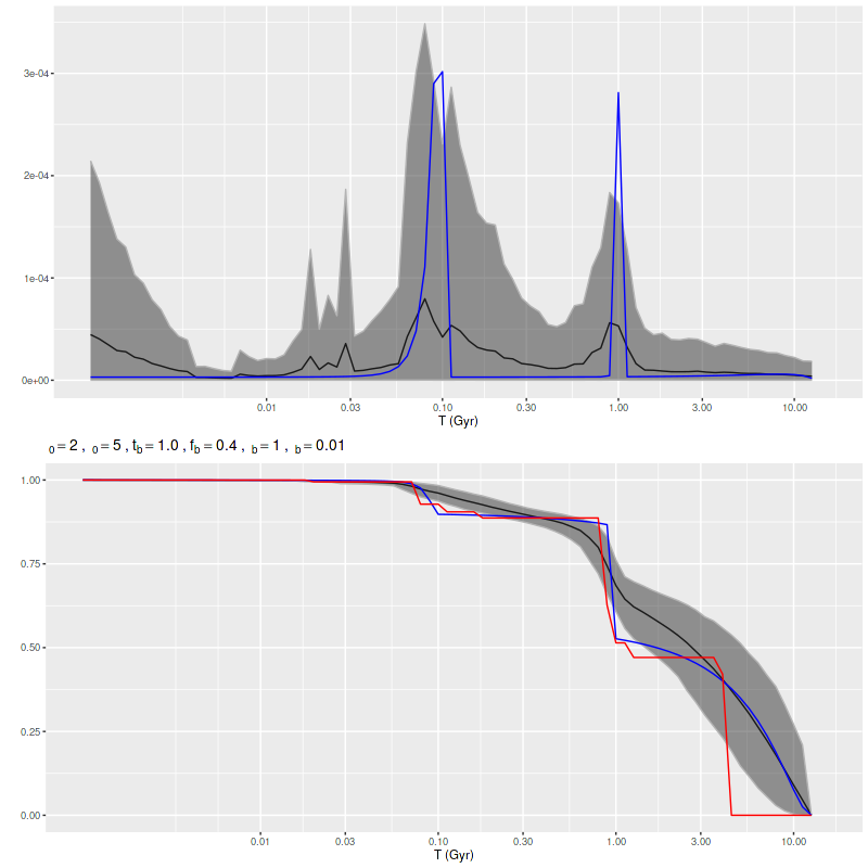
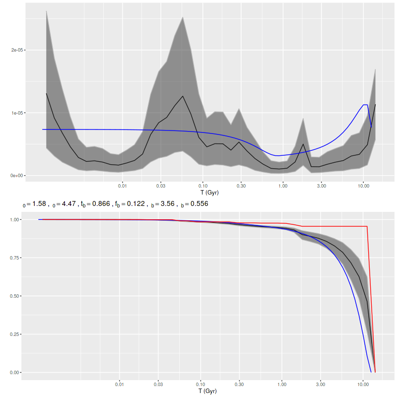
The model star formation history from the same simulated data contains some surprises, and these turn out to be fairly generic features of most model runs. This is a bit of a new graphical display for me. I’ve put the star formation rate history above the mass growth history with the same age scale for each so I can get different views of the same sequence of events. The input model parameters are on a line in between. The blue lines are the input star (mass) formation history. The red line in the second plot is from the preliminary maximum likelihood fit. The black lines and grey ribbons are the marginal means and 95% confidence intervals. Reading from right to left there are several points to note:
The details of the pre-burst SFH are largely lost, although the total mass formed in the model is roughly the same.
The ramp up to the peak of the burst begins sooner and is more gradual than the input. Note that both the input SFR and mass growth are well outside the model confidence intervals in the ramp up period.
Most significantly in my mind at least, the peak of the burst is much later (more recent) in the model than the input. This turned out to be a fairly generic feature of these models.
In this run the post-peak decay is rather steeper on average than the input. In model runs with a rapid input decay the model will usually have a more gradual one.
The input and model SFR eventually converge and the late time model SFH agrees very well with the input, except
There’s an odd upturn in SFR at the very youngest ages (< 3 Myr). This happens to varying degrees in every simulation model run and in all the real data I’ve looked at. It turns out there’s a simple explanation for this. There is virtually no spectroscopic evolution in the relevant wavelength range in the first few Myr of a coeval population’s life. Since the spectra are indistinguishable there is no way to constrain the individual contributions without a more informative prior, and the models are correctly estimating the same marginal distributions for the youngest few populations. Since the time intervals get shorter with decreasing age this produces an apparent upturn in SFR.
Black line and grey ribbon: model results for SFH and MGH. Blue line: input. Red line: MGH from maximum likelihood fit.ProGeny generated SSP model spectra — C3K base models – ages 1-10 Myr, solar metallicityProGeny generated SSP model spectra — C3K base models – ages 1-2 Myr, solar metallicity. Spectra are vertically offset.
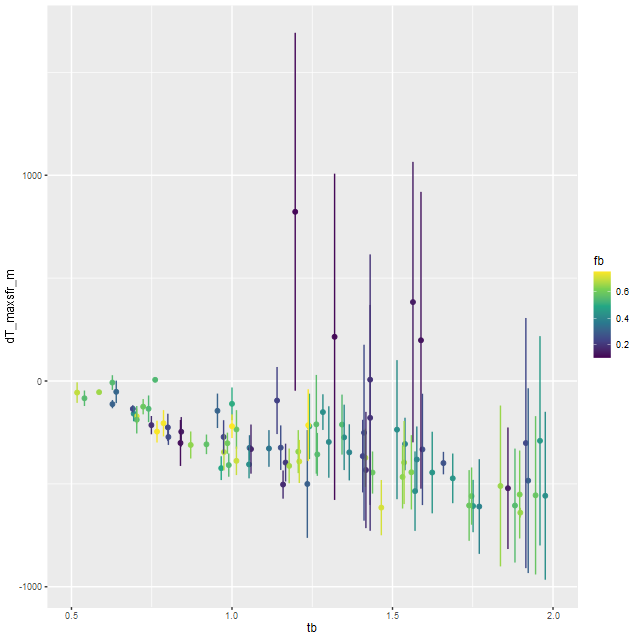
There are two surprises in the simulations I’ve run so far. First is that, like the example above, the time of peak star formation in the model burst tends to be biased downwards (more recent) from the input. The bias gets larger in magnitude with increasing lookback time to burst onset and can be as large as several hundred Myr as seen below. The few outliers here were weak bursts with very large variations in the time of maximum SFR.
Bias in time of peak SFR vs. input burst onset time
The other surprise is that the 95% confidence bands of the model star formation histories, whether viewed as SFR or mass growth histories, fail to cover the inputs for at least some epochs around the time of the burst. In other words the models are saying that the actual input star formation histories are highly unlikely. Why is this?
It’s not, I think, because of any convergence failure. Stan is quite aggressive at flagging potential issues and there were virtually none in any of the model runs. I also don’t think it’s because the model runs were too short. I’ve occasionally gathered much larger samples with longer warmup times as well and except for exploring the tails of the distributions a little more thoroughly there is little change in marginal 95% confidence intervals.
Most of the model runs were done with the reduced size SSP library with just half of the available age bins (0.1 dex intervals). This doesn’t seem to have reduced the real effective age resolution, but in the small number of runs I did with the full set of ages the marginal contributions have larger confidence intervals, so this could increase the coverage.
I suspect though that the prior on the star formation history is having a larger effect than I would have suspected. The main clues here are the maximum likelihood fits. which often produce mass growth histories (the red lines in the plot above and the ones below the fold below) that are rather close to the input MGH, also falling outside the 95% model confidence bands for at least some epochs. In my current workflow the slightly perturbed maximum likelihood solution is used to initialize the Stan model. In most of the model runs the samples quickly move away from the initial values. While the fits to the data are good in all model runs the summed log-likelihood of the sample spectra is always less than the maximum likelihood solution, in the sample shown below by about 7%.
Log-likelihood of posterior samples and maximum likelihood solution for a simulated model run
Below the fold I’ve posted some more cherry picked examples of model star formation histories. A few general comments about them:
The late time star formation rate is generally well captured by the models.
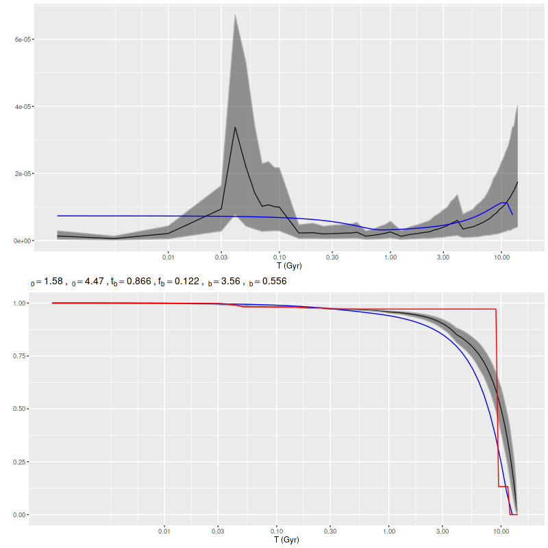
The ancient (pre burst) star formation history is sometimes captured well with weak bursts. Particulary noteworthy is the second example below, which has a recent and weak burst with a gradual ramp up and decay. The entire star formation history is modeled accurately. In the literature there are sometimes references to “outshining” or a “dazzle” effect in (post)-starburst galaxies. This seems to be a real thing.
Early time bursts aren’t necessarily recognizable as such. In some cases the model just shows an extended period of star formation followed by more or less gradual quenching. I believe this is consistent with some claims in the literature, but I don’t care to look for the relevant papers right now.
I’ll conclude with a look at results for all simulation runs (so far) for some of the summary quantities I track. First, the present day stellar mass is on average unbiased but in individual runs there are errors as large as ±0.1 dex. The typical posterior uncertainties are only ~0.01 dex, so the models are consistently too optimistic. I’ve noted this in real data, which shows similar nominal uncertainties with moderately high S/N data.
Not shown here but I did notice a weak dependence on the input burst onset time or time of maximum SFR in the sense that recent bursts tend to underestimate the stellar mass. This is another possible manifestation of the “outshining” effect.
Error in model stellar mass vs. input stellar mass
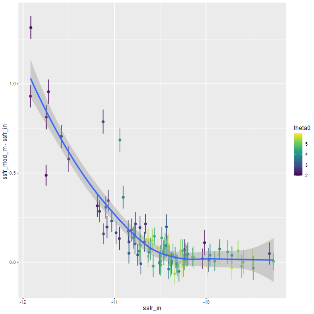
The most dramatic bias is a tendency to overestimate the specific star formation rate when the input SSFR is low. This is also something I’ve seen in real data: as I’ve noted a time or two even the reddest and deadest of ellipticals seem to have a floor of about -11.5 for the estimated SSFR.
One thing I didn’t think about until finishing this analysis is that the contribution estimates tend to be skewed to the right when they’re near 0, so the median might be a better estimate of central tendency than the mean. That might make a (probably) small difference. I will look into this.
Error in model specific star formation rate vs. input SSFR
Finally, there’s a nearly linear relation between the error in the posterior estimate of the optical depth of attenuation and the input. Note also the stratification of the reddening slope parameter δ: at relatively high input optical depths the largest departures have the reddest attenuation curves. I think this behavior is directly related to the prior. Since I don’t think the attenuation is very well constrained by the data I use fairly informative priors on both the optical depth and slope parameter; both priors are truncated normals with a lower bound of 0 for τV and a range of (-0.5,1.2) for δ. This is an easy thing to test simply by changing the priors for these parameters.
Mean and standard deviation of model optical depth – input optical depth vs. input optical depth
I am not quite finished with these simulations. I want to expand the range of input parameters a little bit, and I need to look a little more carefully at subsets of the ProGeny SSP models. The main result so far is that my hopes of timing key events in post-starburst galaxies’ histories were probably too optimistic.
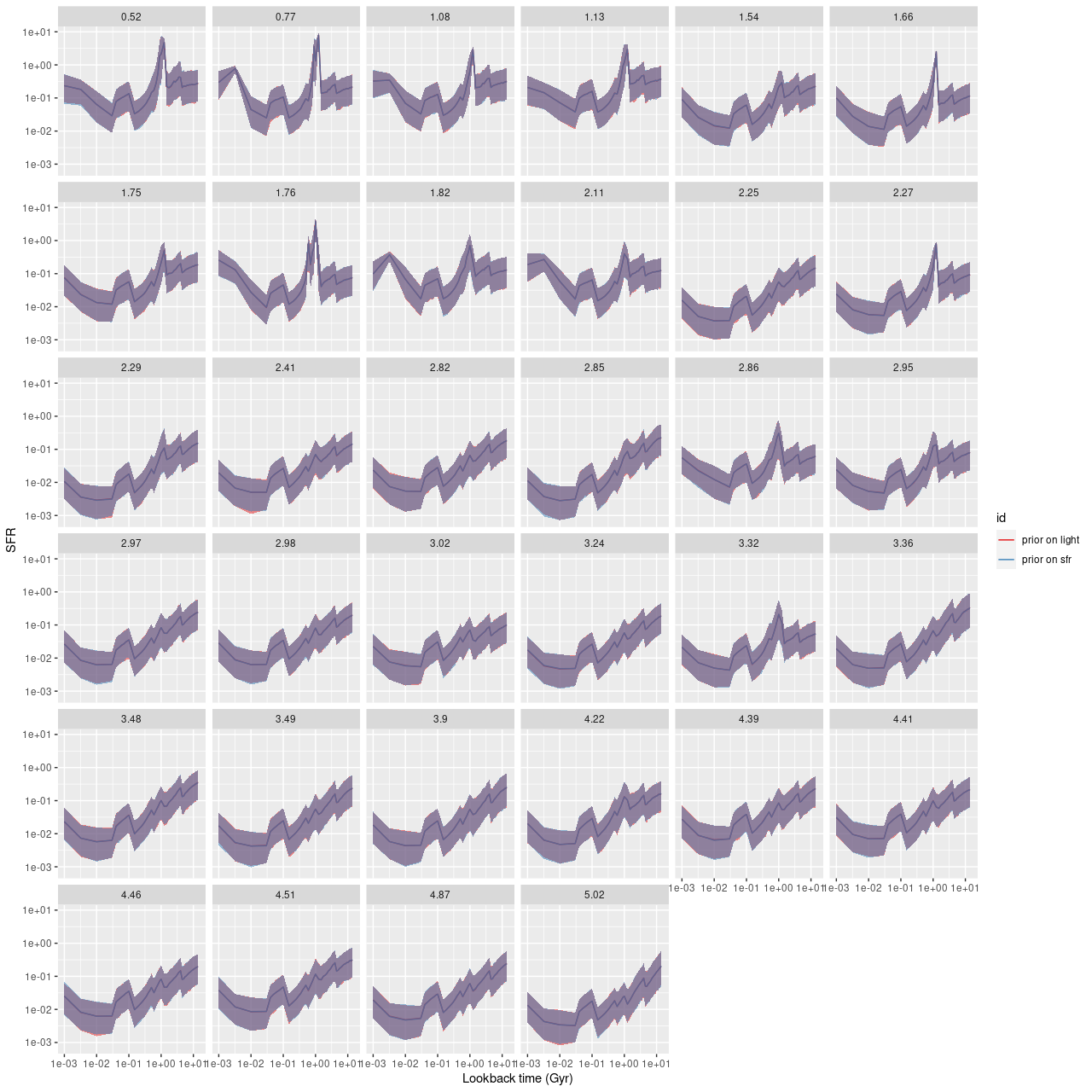
One thing I’ve wondered about for a while is the extent that priors on SSP model contributions affect modeled star formation histories. Previous experience suggests not much at all unless the prior is highly constraining. To be a little more specific in my current workflow I normalize the SSP model spectra to have average flux values of 1 in (approximately) the V band, and also adjust the galaxy fluxes in the same way. In the Stan model the stellar contribution parameters are declared as a simplex, that is a vector with non-zero elements summing to 1. That makes the parameter values the fractional contributions to the (unreddened) galaxy flux at V. My current working code doesn’t provide an explicit prior for the stellar parameters, but they have an implicit proper prior of a uniform distribution on the appropriate dimensional simplex. More technically the prior is a Dirichlet distribution with all concentration parameters equal to 1. Note the marginal distributions aren’t uniform, but they are all the same. One implication of that is that a typical draw from the prior1Stan doesn’t sample from the prior even for initialization, but of course the prior influences the posterior through Bayes’ rule. will have jumps in the star formation rate at exactly the times where the width of the age bins jump, a problem that I’ve noted several times before.
A possible solution to this problem is simply to alter the prior to encourage smoothly varying star formation rate rather than smoothly varying light contributions. It turns out I’ve been feeding my Stan code the data I need to do that: the initial mass in a given model SSP is inversely proportional to the normalization factor applied to the spectrum, and the star formation rate is just the mass divided by the time interval assigned to the SSP. Both of those quantities are passed as data to the Stan model even though they weren’t used in any way previously. I added just 3 lines to the code to change the prior on the stellar contributions. In the “transfored data” section
If I did this right the prior is completely agnostic to any star formation history, whereas the previous implicit prior was completely agnostic to any run of light contributions.
The modified code compiled without complaint and there’s no discernible difference in either execution time or convergence diagnostics.
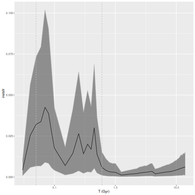
I’ve only run this on one set of galaxy data, from MaNGA plateifu 8565-3703 (mangaid 1-92735). This is one of Schawinski’s “blue early type galaxies,” chosen mostly because the data were binned to just 34 spectra so a complete set of model runs only took a few hours. And, as seen below the other things that don’t change are the modeled star formation histories.
Plateifu 8565-3703 (mangaid 1-92735). Star formation history models with two distinct priors on stellar contributions.
I need to do some more validation exercises, but it appears my long ago conclusion that the choice of prior on the star formation history has little effect was correct. The data dominates the model outcome through the likelihood.
Update
Since I hit publish a few days ago I realized two things. First, the weights I applied to the stellar contributions to “encourage” a smoothly varying star formation rate were inverted. What I should have used was:
The second thing I realized is this makes no difference at all given the form of the prior. The transformation simply maps a point on the simplex to another point on the simplex that has exactly the same probability density since by construction the prior is uniform on the simplex.
So, it should have been expected, and it’s a good thing that it in fact happened that the model runs produced the same results. What happens if I use the following prior, with the weights supplying the parameters for the Dirichlet?
target += dirichlet_lupdf(b_st_s | norm_sfr);
This failed to sample almost always. I’m not entirely sure why, but I suspect this turns a problem with relatively simple geometry at least with regards to the prior to one with a complex and troublesome geometry.
This little experiment actually told me nothing about the effect of priors on model star formation histories. Two of the priors are actually the same, and the third fails for reasons that aren’t completely clear. I may experiment with different forms of prior. I’m still, of course, looking for a new SSP model library.
Instead of trying a systematic investigation I’m just going to go through each IFU and discuss whatever I found interesting, with no particular theme in mind. I still don’t really know what I’m going to find since it’s been a while since I looked at model results. Besides modeling star formation histories for each spectrum I calculate summaries in the form of posterior marginal means, standard deviations, and a few quantiles for a large number of quantities. Some of these are highly model dependent such as 100 Myr averaged star formation rates and specific star formation. Some are only weakly model dependent, such as emission line fluxes1These depend on correction for absorption, but we don’t need a believable star formation history for that, just a reasonable template match. One thing I haven’t looked at much is stellar metallicities and especially their evolution in the models. There are always contributions from all metallicity bins at all times in my models, and how to interpret them or whether even to try still puzzles me. I am starting to look more seriously at strong emission line metallicity estimates. The estimator proposed by Dopita et al. (2016) based on [N II], [S II], and Hα seems especially promising since they’re usually detected with reasonable precision in SDSS spectra.
So, the plan is to look at each IFU, working my way outward in the disk in the same order as my second post in this series.
plateifu 9677-12705 (mangaid 52-4)
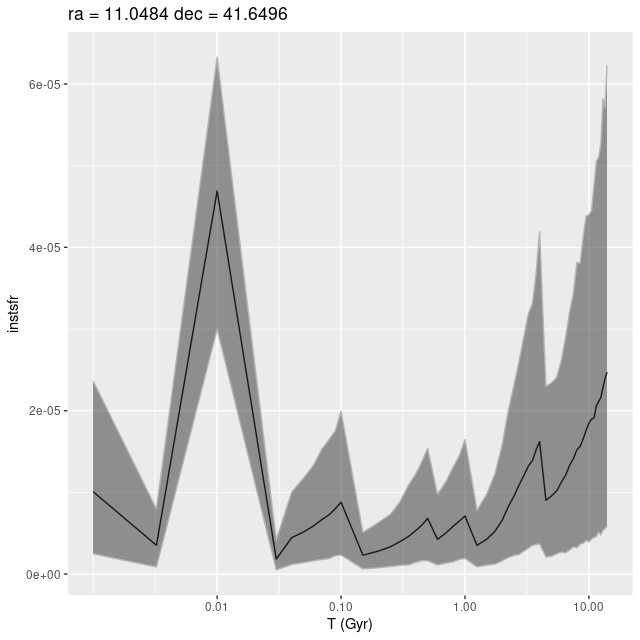
This is the innermost IFU with a projected distance from the nucleus of 1.9 kpc. According to Walterbos and Kennicutt (1988) the effective radius of the bulge is 2 kpc, so a significant fraction of the light is coming from bulge stars.
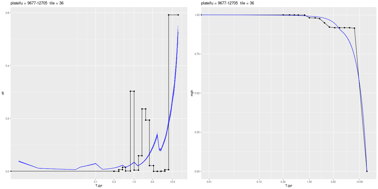
What’s most interesting about this IFU is what it lacks, which is any significant star formation. I also saw little spatial variation in model star formation histories, so I’ll simply repeat the IFU wide history compared to the nearest PHAT tile:
Innermost IFU 9677-12705 SFR and mass growth histories compared to models for nearest PHAT region.
This region had the most rapid initial stellar mass growth and conversely the steepest decline in SFR of any of the MaNGA IFU’s, which is completely consistent with the consensus “inside out” growth paradigm.
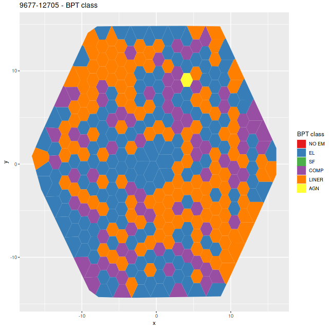
One other moderately interesting result is that despite the lack of young stars there are detectable emission lines throughout with a mix of “LINER” and composite like line ratios from the [N II]/Hα vs. [O III]/Hβ diagnostic and the classification scheme of Kauffmann with Schawinski’s addition of the LINER/AGN divide. As is well known by now LINER (and presumably “composite” although I haven’t seen literature on the issue) emission can be spatially extended and does not at all necessarily indicate ionization by an AGN. M31 has widespread emission from diffuse ionized gas. About 14% of all binned spectra had line ratios in these categories and “AGN” like, and 90% of the LINER-like spectra are in this IFU. A similar fraction of spectra have star forming emission line ratios, which reflects the patchy nature of star formation in M31.
plateifu 9677-12705 – BPT class per [N II]/Hα vs [O III]/Hβ diagnostic
plateifu 9677-6102 (mangaid 52-3)
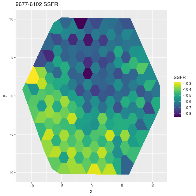
There’s little to say about this one. The entire IFU is offset by a small amount from some GALEX UV bright sources and there are no objects in any of the catalogs I’ve loaded within the footprint. The only prominent feature is a very prominent dust lane that covers the southeastern half of the IFU. Oddly, the estimated specific star formation rate tracks the dust rather closely.
plateifu 9677-6102 (M31 inner disk). Specific star formation rate
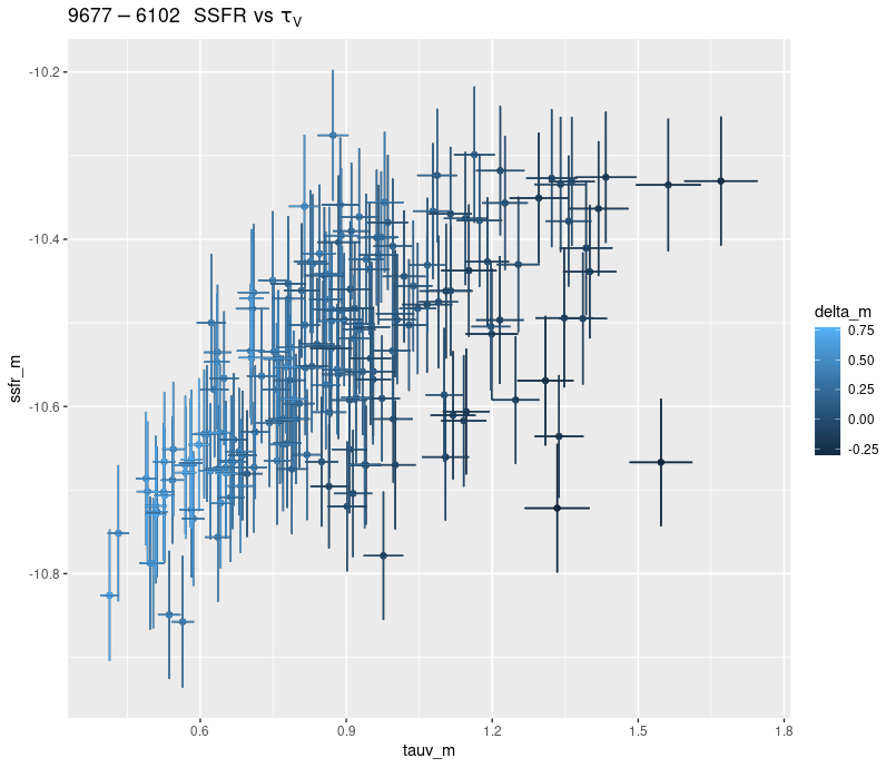
There’s a clear correlation between SSFR and optical depth of attenuation, and also with the “tilt” of the attenuation relation:
plateifu 9677-6102 (M31 inner disk). Specific star formation rate vs. dust optical depth.
Whether this is meaningful or a modeling artifact I can’t say at this point. I kept my simple single component dust model for these runs even though M31 is known to have both a foreground screen and embedded dust.
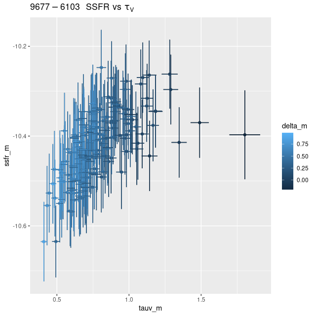
plateifu 9677-6103 (mangaid 52-2)
This again is in a nearly featureless area except for a prominent dust lane, with no sources in any catalog I consulted. The entire IFU lacks significant emission and there is no evidence in the models for significant recent star formation. Oddly, there’s a very similar relation between model specific star formation rate and model optical depth:
plateifu 9677-6103 (M31 inner disk). Specific star formation rate vs. dust optical depth.
plateifu 9677-12701 (mangaid 52-8)
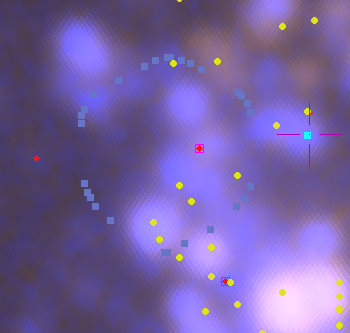
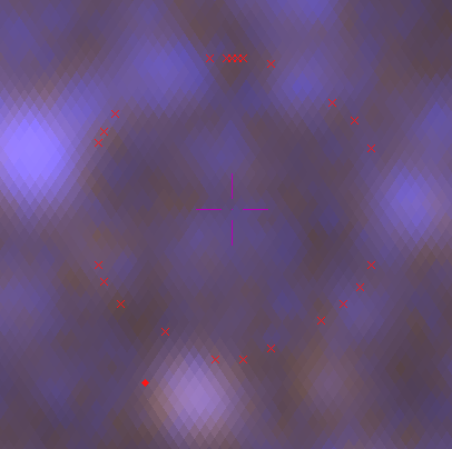
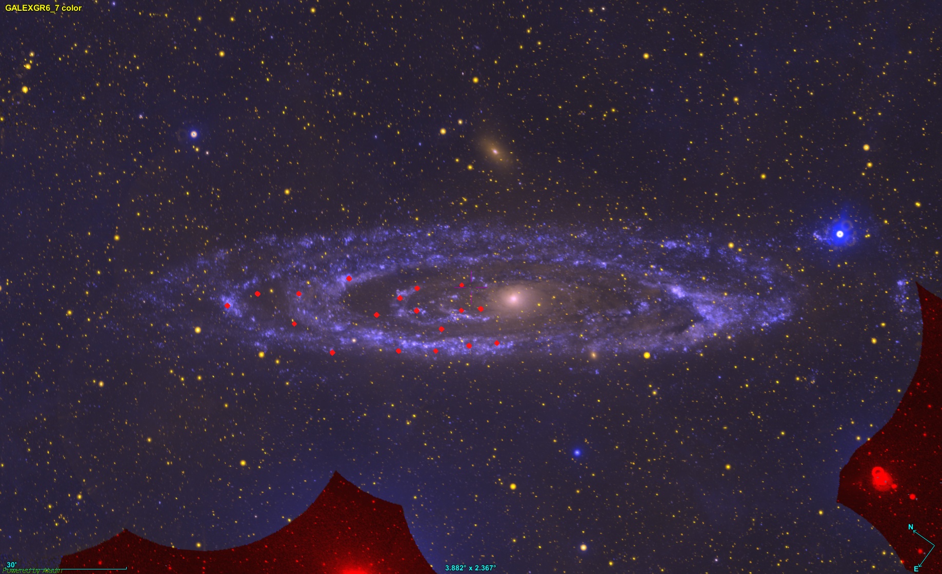
This is the closest IFU to the nucleus that lies within a significant spiral structure as seen by GALEX. The thumbnail below shows its position overlaid on the false color GALEX image available within Aladin. The IFU appears to lie in a spur off a spiral arm a little farther out2There doesn’t seem to be a strong consenus about the overall spiral structure of M31. All modern authors agree that the “10 kpc ring” is a complete ring, with a split in the south not too far from the projected position of M32. I’ve also seen references to 6 and 16 kpc rings, but others claim that various classes of young objects are strung out along a pair of logarithmic spirals. This idea goes back to early 1960’s work by Baade and Arp. I will just note IFU’s in UV bright areas in GALEX since this seems to be the best tracer of recent star formation and a number of discrete UV bright sources are visible within its footprint, which is marked with the irregular set of blue symbols. Also shown are cataloged positions of H II regions (yellow dots), red supergiants (red diamonds), and an OB association (blue square)3data sources are given in the last post. All of these are available through Aladin’s data collection.
Thumbnail of plateifu 9677-12701 (M31 inner disk) overlaid on GALEX false color image. Yellow dots: cataloged H II regions. Red dots: cataloged red supergiants. Blue square: OB association.
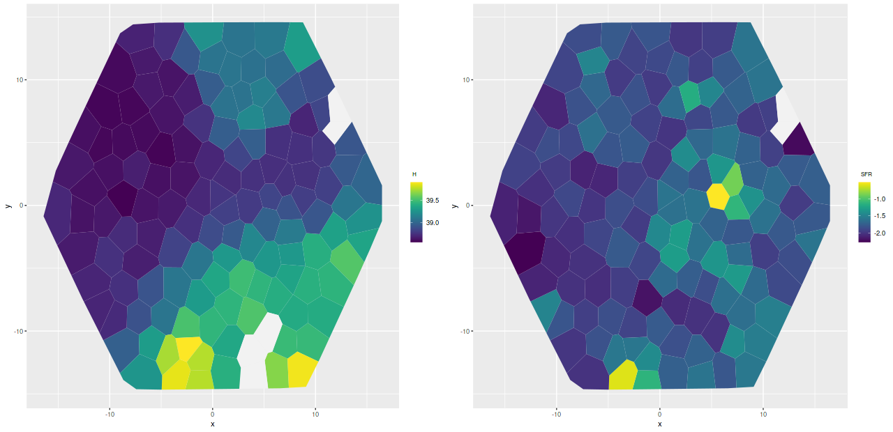
Let’s look at a couple of maps. The blank area at upper right was masked due to a likely foreground star. The spectra in the chain of blank areas at bottom had Hα partially masked. Units in the Hα luminosity density map are log10 ergs/sec/kpc2, uncorrected for attenuation. Units of the SFR density maps are log10 M☉/yr/kpc2.
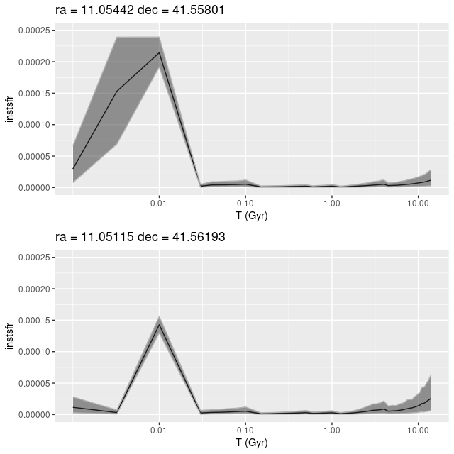
To a pretty good approximation regions that are relatively bright in Hα track the UV bright areas and cataloged H II regions. There are two areas that stand out as having much higher than average SFR density. One, at lower left, coincides with a bright H II region. The other one, at center right, has low Hα luminosity but lies right on the cataloged position of a red supergiant. The presence of an evolved star and absence of emission suggests that star formation has recently (in the last ~70 Myr, say) ended in that area. Comparing the model star formation histories the region with little Hα emission does show a sharp drop-off after a peak at 10 Myr lookback time:
plateifu 9677-12701 (M31 inner disk) – model star formation histories for 2 star forming regions.
One other thing I’ll just note for now is that regions with the highest star formation rate tend to have neighboring regions with higher than average star formation as well. These seem to occur in clumps or chains a few 10s of parsec in size. I will get, eventually, to some more dramatic examples.
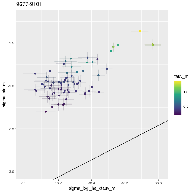
plateifu 9677-9101 (mangaid 52-9)
This and the next IFU are in a spiral segment that some authors call the “6 kpc ring,” but the GALEX false color image shows no very bright UV sources and there are no cataloged young objects within the footprint.
9677-12701 GALEX cutout
One mildly interesting result is that the modeled 100 Myr SFR density correlates rather strongly with Hα luminosity density, but an order of magnitude higher than predicted from Calzetti’s calibration. All of the emission in this region appears to be from diffuse ionized gas as there are no cataloged discrete sources of emission, and no regions with starforming line ratios. A literal interpretation of this, which might even be true, is that star formation has ceased in the recent past.
plateifu 9677-9101 (M31 inner disk). Star formation rate density vs. Hα luminosity density.
plateifu 9677-12704 (mangaid 52-5)
This is also in the 6 kpc spiral feature but in an area with no bright UV sources and that appears to be heavily dust obscured in optical images. Since I don’t have anything very interesting to say about this region I’ll just post the modeled star formation history for the region within the IFU footprint with the highest modeled SFR density. This is near the western edge of the IFU and isn’t associated with any cataloged young objects.
plateifu 9677-12704 (M31 inner disk). Star formation rate history for a region within the IFU footprint with the highest modeled recent SFR.
The region with the highest Hα luminosity is near the southwest edge and covers the position of a cataloged planetary nebula. The emission line ratios are inconsistent with a starforming region, falling in Kauffmann’s “AGN” region.
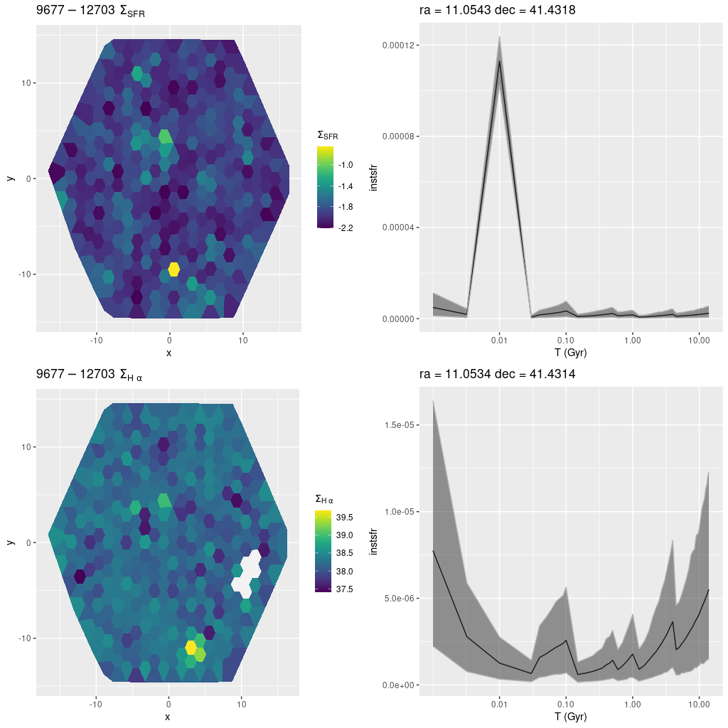
plateifu 9677-12703 (mangaid 52-6)
This and the last IFU are in an inter-line region between the 6 and 10 kpc structures as seen by GALEX, but with lots of diffuse starlight and relatively little dust. Emission lines are weak or undetected throughout, but there is a cataloged H II region near the southern edge. The peak in Hα luminosity density is easily seen in the map below in the bottom left pane. The region with the highest SFR density is displaced by ~10 pc. from the region with highest Hα luminosity. Interestingly, the SFR models show significant differences in recent histories: the region with highest SFR shows a very sharp and short lived peak at ~10 Myr, while the highest Hα luminosity region is still growing in SFR (per the model). Again, I hesitate to take these model histories too literally, especially at the youngest ages, but these are consistent with the fact that ionized gas emission will fade rather rapidly as the most massive stars in a region evolve away from the main sequence.
plateifu 9677-12703 (M31 inner disk). (TL) SFR density (100 Myr average) (BL) Hα luminosity density. (TR) SFR history for the region with highest SFR density. (BR) SFR history for the region with highest SFR Hα luminosity density.
plateifu 9678-12705 (mangaid 52-21)
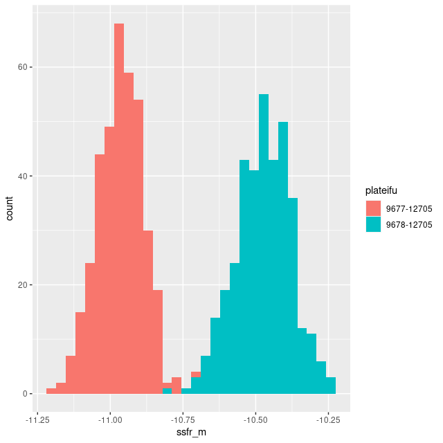
I don’t have much to say about this one either. It lies in a region that’s almost completely blank in the GALEX imaging, with a rather uniform sprinkle of stars in PHAT and the DSS2 image displayable in Aladin. Ionized gas emission is weak or undetected throughout. For the sake of having a graph to display here is a histogram of the per spectrum mean specific star formation rate (100 Myr average as always) comparing this IFU to the innermost one — plateifu 9677-12705.
Distributions of mean specific star formation rate in two MaNGA M31 IFU’s
I hope to finish off M31 in one or at most two more posts. Next up are IFUs that fall in or near the 10 kpc ring, followed by the outer disk.
After a fairly long break I want to get back to M31 and MaNGA for one, or perhaps several posts and take a more detailed look at my model results. I still haven’t decided where I’m going to take this investigation. I may examine every IFU or just the ones that I found most interesting, and I’m not sure which of the many quantities that I estimate I’ll discuss. Besides my models I’ve retrieved a number of catalogs of interesting objects using Aladin. These include in particular H II regions (Azimlu et al. 2011), OB associations (Magnier et al. 1993), and red supergiants (Ren et al. 2021). All of these are products of recent or ongoing star formation. There are of course a huge number of catalogs of just about every type of astronomical object found in galaxies, and I may examine some more depending on what interests me.
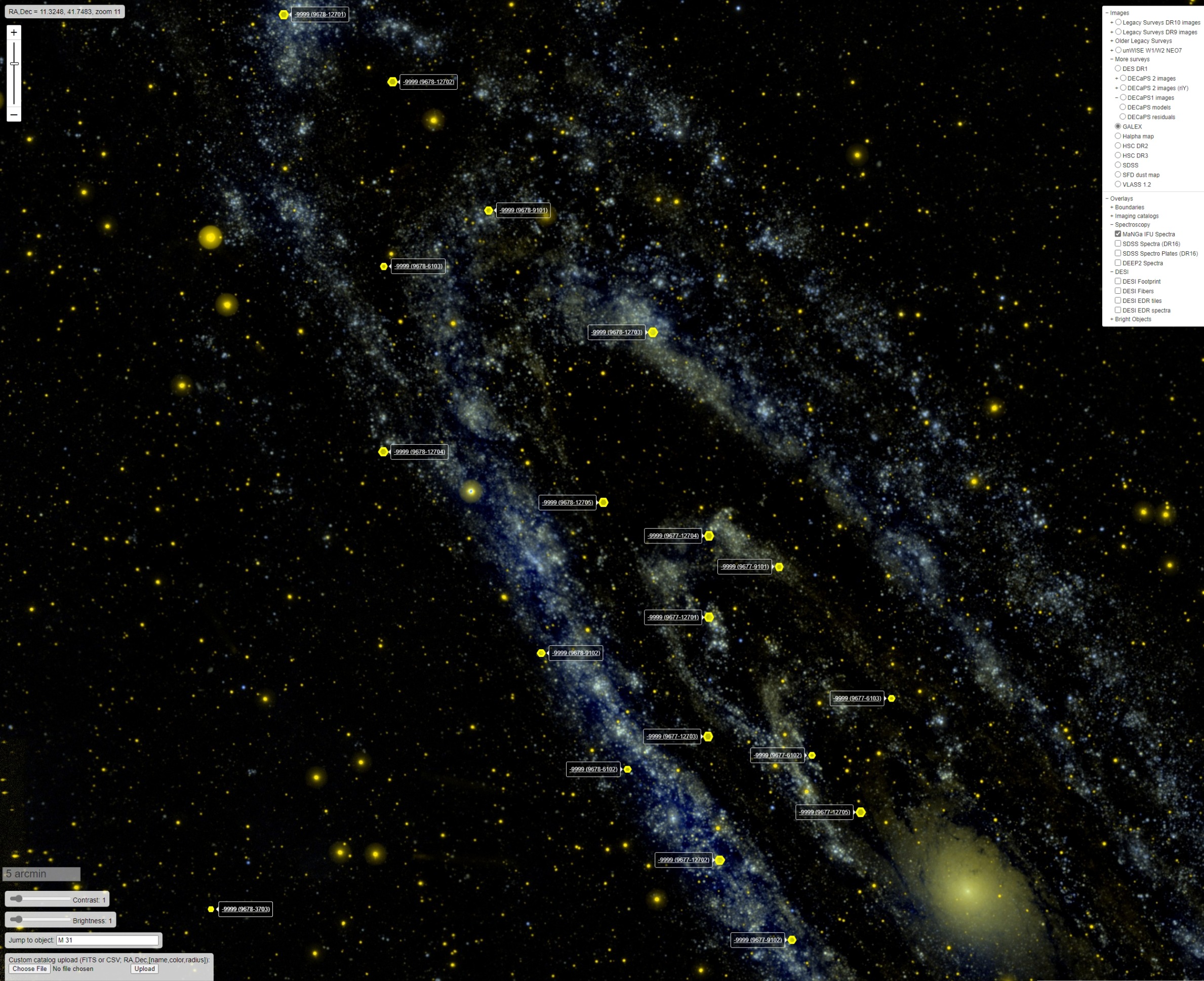
For orientation here’s a screencap of the Legacy Survey sky browser’s false color GALEX image of the northern half of M31 with the IFU positions overlaid and labelled with MaNGA’s plateifu identifiers. As a reminder these are all located within the PHAT survey footprint and specifically within the region for which star formation histories were estimated by Williams et al. (2017).
Screen capture of Legacy Survey Galex image of M31 with MaNGA IFU overlay
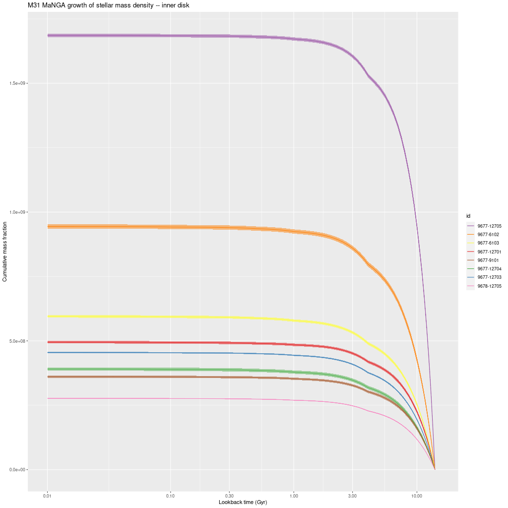
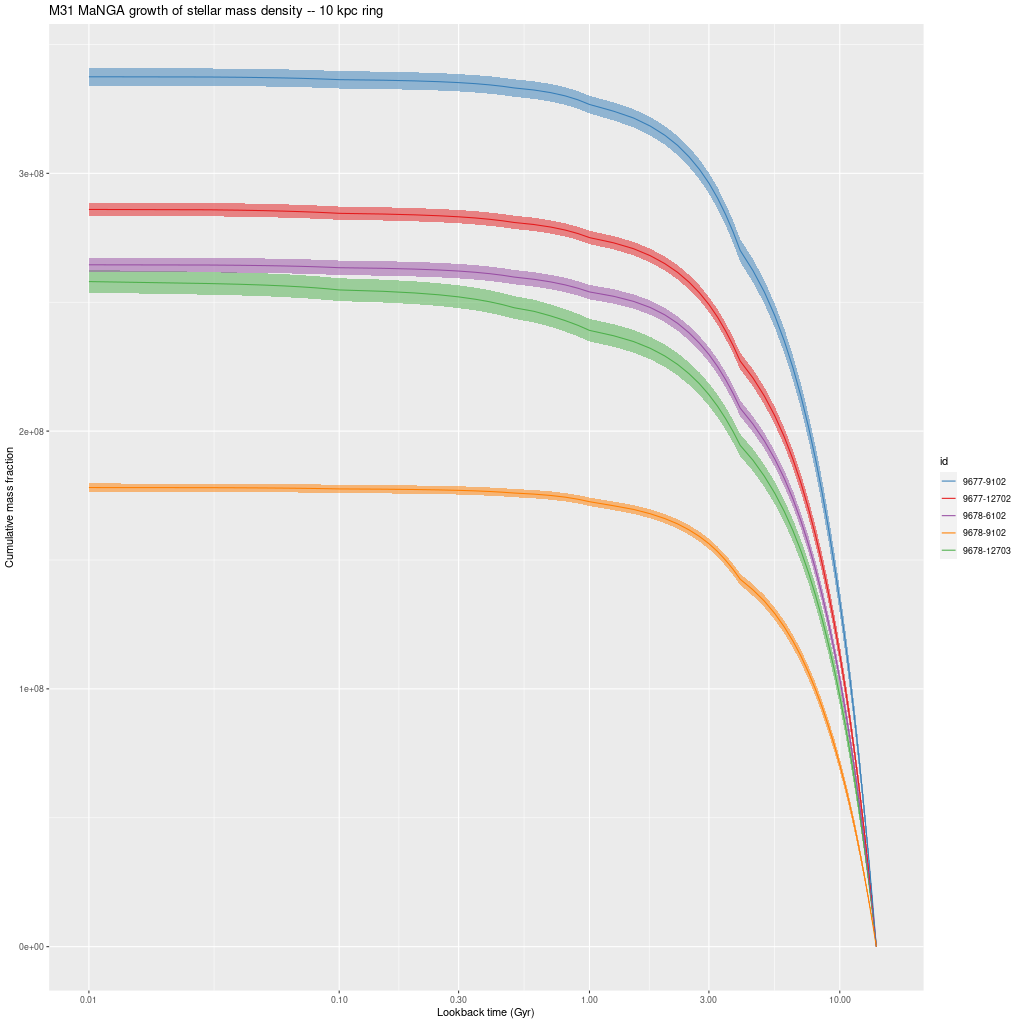
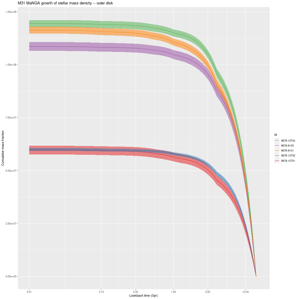
Before getting to individual IFU’s here is one more set of IFU-wide results. The following three graphs are model mass growth histories in units of present day solar mass per kiloparsec2. These are uncorrected for projection effects.
There are a couple interesting points here. There’s a clear stratification of mass density with projected radius, with about a factor 30 decline from the innermost to outermost IFU. This is in fairly good agreement with Williams’ estimate in their Figure 14.
The other thing to note is that all regions had most (> 55%) of their stellar mass in place by 8 Gyr ago and 92-99% in place by 1 Gyr ago. The largest fraction of recent star formation is in the IFU 9678-12703, which is very close to the region with the highest SFR in this half of the galaxy. There is also a trend towards later mass build up with increasing radius, which is completely consistent with the “inside-out” growth paradigm. The outermost IFU, 9678-12701 at about 16kpc radius has formed about 5% of its present day stellar mass in the past Gyr.
As I said in the previous post I don’t see clear evidence for a widespread burst of star formation that’s widely believed to have occurred around 2-4 Gyr ago. A confounding factor in my models is that they invariably show jumps in SFR at times when the interval between SSP model ages change and the two oldest of these occur at 1 and 4 Gyr, so this produces a possibly spurious period of apparently accelerated star formation. I hope to find (or perhaps produce) a set of SSP models with a better age distribution this year.
Growth of stellar mass density – inner disk M31 MaNGA IFU’sGrowth of stellar mass density – M31 MaNGA IFU’s in 10 kpc ringGrowth of stellar mass density – outer disk M31 MaNGA IFU’s
I think I’m going to hit publish now and resume with inner disk IFU’s next time.
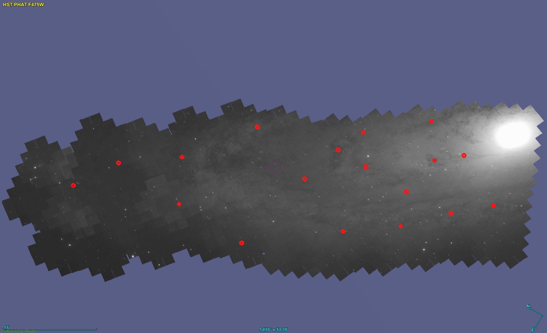
One of the ancillary programs (with principal investigator Julianne Dalcanton) in the final MaNGA release targeted 18 fields in the disk of the Andromeda galaxy M31. The targets were selected from within the footprint of the “Panchromatic Hubble Andromeda Treasury,” aka PHAT1not my coinage., also with PI Dalcanton. The initial PHAT survey description was in Dalcanton et al. (2012) and was followed by a lengthy series of papers. Especially relevant for this discussion are two papers describing estimates of the recent and ancient star formation histories of the disk outside the area dominated by bulge light: Lewis et al. (2015), “The Panchromatic Hubble Andromeda Treasury. XI. The Spatially Resolved Recent Star Formation History of M31” and Williams et al. (2017), “PHAT. XIX. The Ancient Star Formation History of the M31 Disk.” For reference here is a mosaic of HST images in the F475W filter with the IFU locations overlaid:
Mosaic of HST F475W images of PHAT study region with M31 MaNGA IFU positions overlaid
Zooming out to show the whole disk here they are overlaid on a false color FUV+NUV image from GALEX, which gives a pretty good picture of where stars are actually forming:
GALEX false color NUV+FUV image of M31 with MaNGA IFU positions overlaid – screencap from Aladin
This data set provides an excellent opportunity to compare my SFH modeling code to a completely different, more direct, method of inferring star formation histories namely counting resolved stars in color magnitude diagrams. I recently completed model runs for all 18 IFU’s with the same Voronoi binning of stacked RSS spectra, the same modeling code and SSP model spectra as I’ve used for a while now.
There’s no redshift listed in the DRP catalog; NED gives a heliocentric redshift of -0.001, but for purposes of calculating intrinsic quantities I need the “Hubble flow” redshift. I adopted a distance of 761 (± 11) kpc or distance modulus of (m-M)0 = 24.407 from Li et al. (2021), which is the most recent and according to the authors most precise determination to date. With my adopted Hubble constant of H0 = 70 km/sec/Mpc this makes the Hubble flow recession velocity 53.27 km/sec or zdist = 0.0001777. The angular scale is 3.69 pc/arc-second. This distance estimate is a few percent smaller than the PHAT team authors and most other recent literature I reviewed, but fortunately most other sources of uncertainty are much larger.
An issue I noticed early on was the modelled values of the optical depth of attenuation were right at 0 for almost all spectra with only a few much larger exceptions. A quick check of the metadata showed that the values adopted for the foreground galactic extinction almost certainly were taken from the SFD dust maps which faithfully capture the intrinsic dust content of M31 albeit at rather low resolution. These hugely overestimate the actual foreground galactic extinction and that has multiple undesirable consequences. So, I assigned a single extinction value of E(B-V) = 0.055 to all IFU’s, consistent with the NED value of AV = 0.17 mag. The preliminary runs were redone with the newly adopted extinction value.
After binning to a minimum mean SNR of 5 there were 2,624 spectra in the 18 IFUs, of which I ran models for 2,621. Three spectra had apparent foreground stars, although one of those might actually be a red supergiant in M31. The fibers are basically sampling star cluster size and stellar mass regions so a single extremely luminous star could potentially affect a spectrum.
I’m only going to show a few summary results for the entire sample in this post. My goal is to do a more detailed quantitative comparison to (at least) the SFH models of Wilson, for which there are extensive results tabulated. There are of course many catalogs of interesting objects within M31, and I plan to look at some of them.
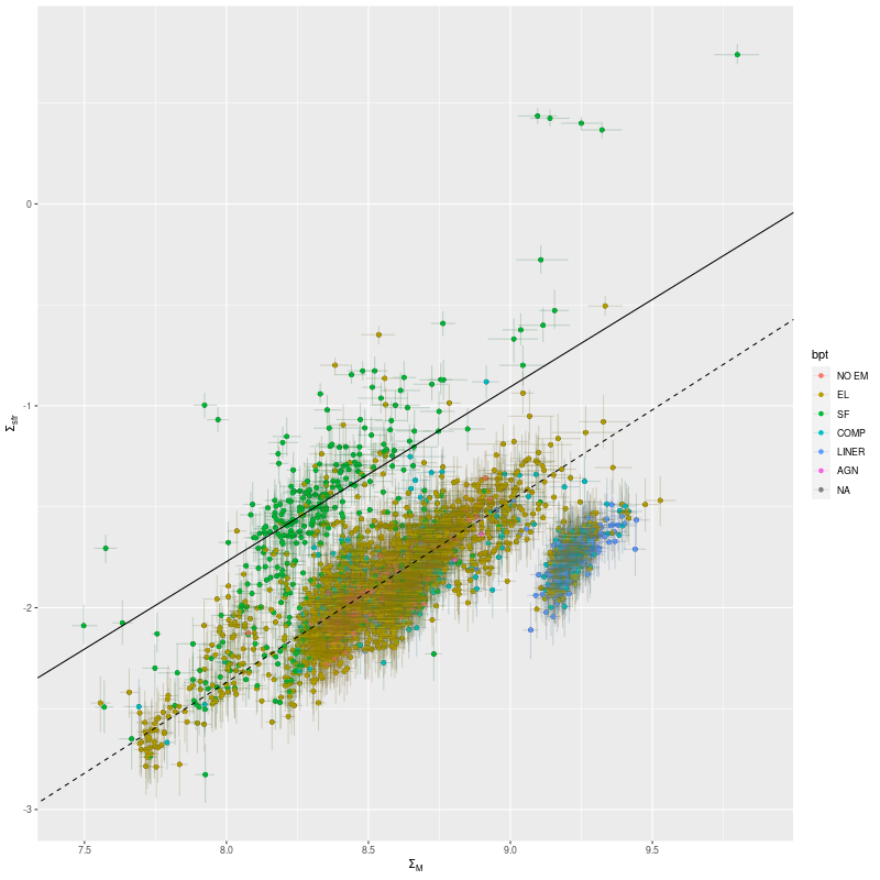
First, here is a plot of the (100 Myr averaged) star formation rate density against stellar mass density, color coded by BPT diagnostic. The solid line is my estimate of the “spatially resolved star forming main sequence” based on a small sample of non-barred spiral galaxies. The dashed line is the estimate of Bluck et al. (2020), which I commented previously appears to mark approximately the location of the green valley at least with regard to my models. A striking feature of this plot is the apparent stratification into at least three distinct groups that can be interpreted as starforming, quiescently evolving, and passively evolving. I suspect this observed stratification is just the result of hand picking a small number of “interesting” regions. Most or perhaps all of the points in the passively evolving group are in the IFU closest to the bulge, while most of those along and above the SFMS lie near the most vigorously star forming regions in the PHAT footprint. Especially noteworthy are 5 outliers that are well above any others in the plot in terms of SFR density. These are all in the same IFU (plateifu 9678-12703) which is located within the largest star forming region in that quadrant of the “10 kpc ring.”
100 Myr average star formation rate density vs. stellar mass density for 2621 binned spectra in M31 disk. Solid and dashed lines are my and Bluck’s central estimates of the “spatially resolved star forming main sequence.
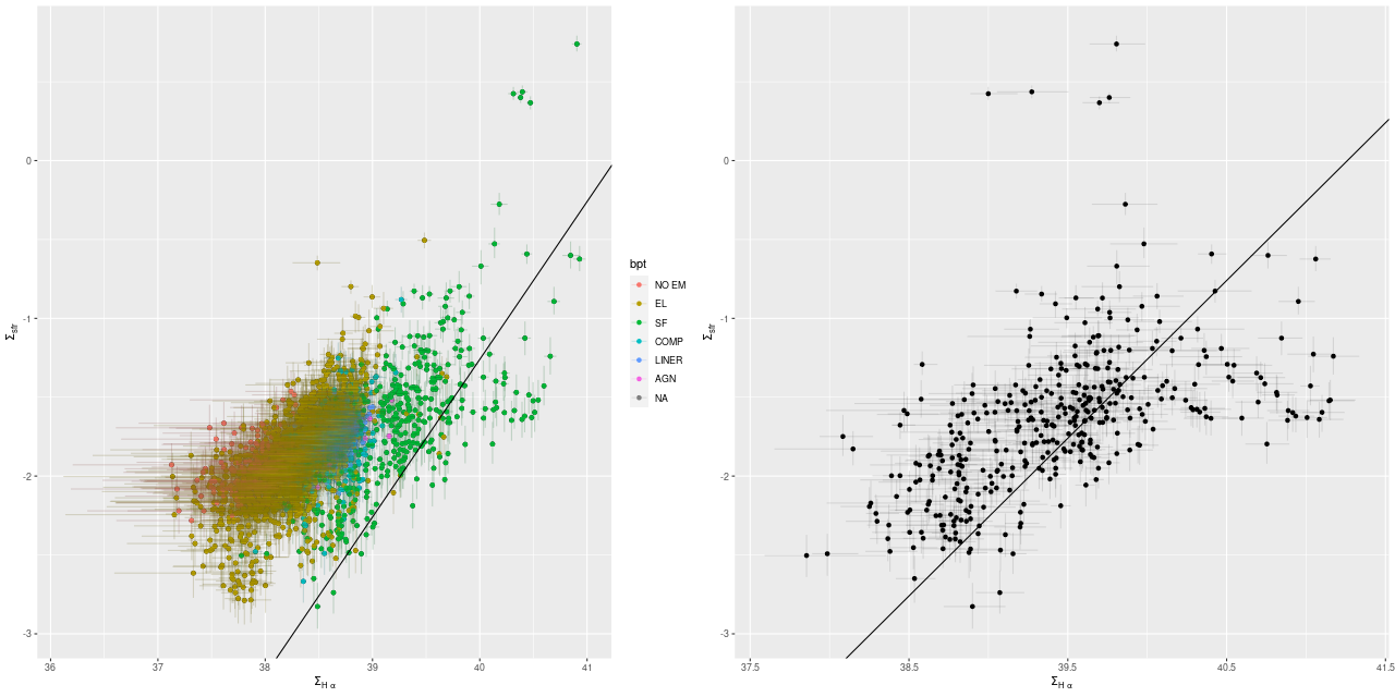
Next are plots of star formation rate density against Hα luminosity density. The left panel is for all spectra color coded by BPT diagnostic, with Hα adjusted by the modeled amount of stellar attenuation. The right panel shows regions with star forming BPT diagnostics only, with Hα corrected by the observed Balmer decrement. The solid line in both panels is Calzetti’s calibration of the Hα – SFR relationship. The relationships plotted here are consistent with what I’ve seen in other MaNGA samples and with published values, which is encouraging.
Star formation rate density vs. Hα luminosity density for 2621 binned spectra in M31 disk. (L) Emission corrected for modeled stellar attenuation. (R) For regions with star forming emission line ratios only: emission corrected from estimated Balmer decrement.
The obvious point of comparison to my models are the detailed star formation histories in the two PHAT papers mentioned at the top. Unfortunately there is no detailed tabulation of model results in the paper by Lewis et al. The paper by Williams et al. has extensive tables, but there are still a few obstacles to detailed comparisons which I will discuss next time.
A few more items from my handwritten notes that I want to get in pixels. I have never previously tried to correct surface densities for inclination in disk galaxies, but for comparison purposes and because of the large inclination of M31’s disk I need to do so here. I adopted an inclination angle of 77°, so a 1″ radius fiber covers a 3.69 x 16.4 pc (semi major and minor axes) elliptical region, or 190 pc2. Densities need to be adjusted downward by a factor 4.45 or -0.648 dex2This adjustment was not made in the plots above. Since these are plots of densities against densities all points would just shift downwards along lines of slope one..
In order to achieve 100% coverage of the IFU footprints the exposures were dithered to three different positions with overlapping fiber positions. Comparing the area in fibers to the area in spaxels in the cubes the overfilling factor averages 0.217 dex or 65%. The total area in all cubes is 10,731 arcsec2, or a deprojected area of 0.65 kpc2. The most distant IFU from the nucleus is at a projected radius of about 16 kpc. A simple extrapolation to the ≈800 kpc2 area of the disk within that radius is probably unsafe.
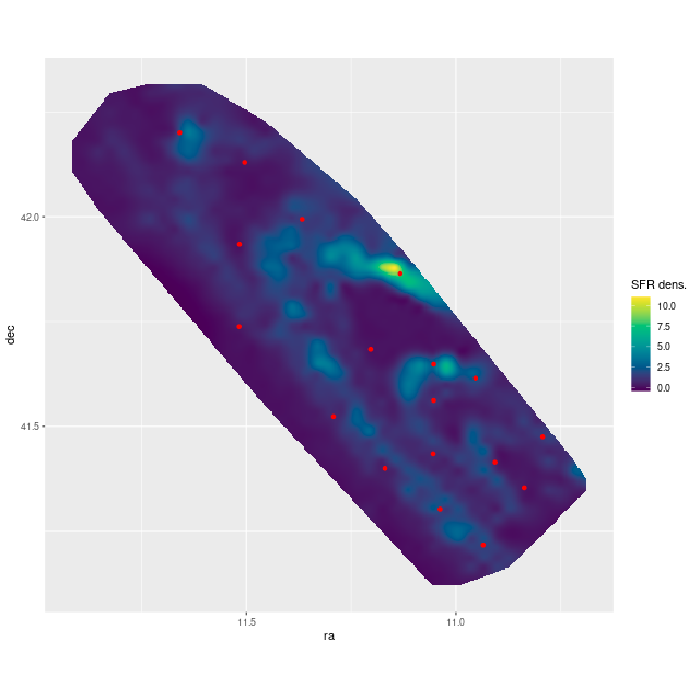
One final map to anticipate the next post(s). Wilson provides tables of model star formation rates for 16 age bins, 826 regions, and 4 different sources of isochrones including the same BASTI isochrones I use. The complete data set is available through Vizier. In the plot below I created a map of the recent star formation rate density interpolated to nominal 10″ resolution from their Table 2 models with BASTI isochrones. This should be compared to their Figure 16 (they use logarithmic scaling).
Current (300 Myr average) star formation rate density in the PHAT footprint per models of Wilson et al. (2017) with positions of MaNGA IFUs overlaid.
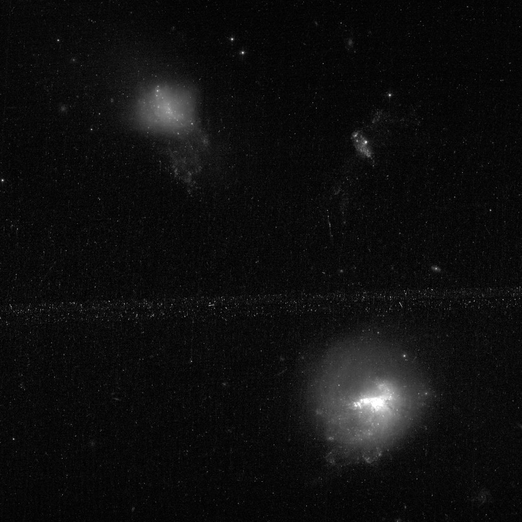
The Hubble Space Telescope “gap filler” program “Gems of the Galaxy Zoos” (proposal ID 15445, PI William Keel) had several prospective targets that I played a small role in selecting, and this recent HST observation was one of them. The actual target was the small disturbed galaxy at top left, which I will refer to as MCG +07-33-040. I don’t know if it was fortuitous that the larger and brighter UGC 10200 was also imaged in the same ACS field, but these are clearly interacting or at least have in the recent past, as is the small system in the upper right, which is identified as a blue compact galaxy with redshift z=0.00556 in Pustilnik et al. (1999). I’m going to focus on the top left galaxy in this post.
Galaxies UGC 10200 (lower right) and MCG +07-33-040 (upper left). HST/ACS, F475W filter. Proposal ID 15445, PI Keel.
What interested me wasn’t the galaxy image so much as its SDSS spectrum, which has three interesting characteristics:
SDSS spectrum of central part of MCG +07-33-040
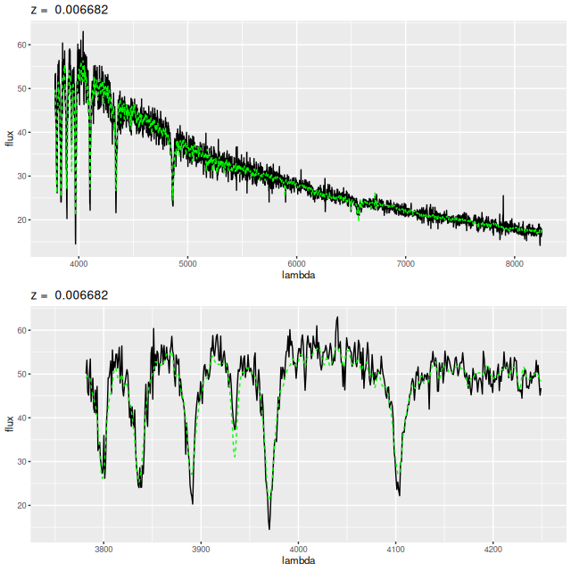
First, this is a classic post starburst galaxy spectrum with extremely strong Balmer absorption lines1My code measures the Lick index HδA as an exceptionally strong 8.06 ± 0.41 Å. and no obvious evidence of emission. In fact, although this designation isn’t used much anymore, it’s actually a classic “A+K” spectrum which reverses the usual “K+A” terminology to indicate the light is dominated by early type (i.e. young) stars. Second and third, the spectrum was misclassified as coming from a white dwarf star, and the redshift was erroneously estimated as around 0.004 which was the maximum allowed for stars in the SDSS data reduction pipeline. Using a variation of the code that I use to measure redshift offsets I get a robust value of z = 0.006682 ± 9E-06
Template fit to SDSS spectrum of MCG +07-33-040
This is almost exactly the same redshift as its nearby companion UGC 10200 (also in the HST image above), which has a securely determined z = 0.00664
SDSS spectrum of central region of UGC 10200
For the rest of this post I’m going to assume the Hubble flow redshift is the measured one, which with my adopted cosmological parameters2which for the record are H0 = 70 km/sec/Mpc, Ωm = 0.27, Ωλ = 0.73. make the luminosity distance 28.8 Mpc, the distance modulus m-M = 32.3 mag, and the angular scale 138 pc/” or about 7 pc per ACS pixel. The projected distance between the centers of the two bright galaxies in the HST image is about 96″ or 13.2 kpc.
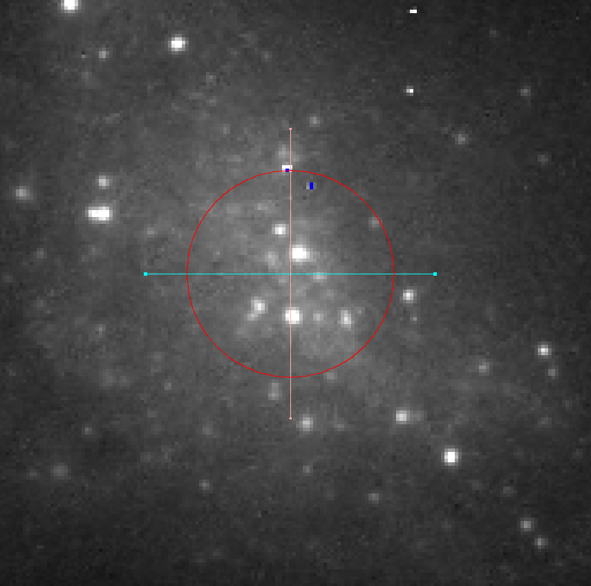
I spent some time last weekend downloading and starting to learn the software Aperture Photometry Tool (APT), which is interactive software for manually performing aperture photometry. Zooming in on the center of the presumed post starburst galaxy I located the reported position of the SDSS fiber as closely as I could. In the screenshot below the aperture radius was set to 30 pixels, the same size as the SDSS spectroscopic fibers. I measured the F475W AB magnitude to be 17.90 ± 0.013 without sky subtraction, which is close enough to the SDSS g band fiberMag estimate of 18.05. The SDSS g band Petrosian magnitude estimate is 15.16, so the fiber contains about 7% of the total galaxy light.
Central region of MCG +07-33-040 with position and size of SDSS fiber overlaid. Screenshot from APT
A striking feature of the HST image is there are many point-like symmetrical objects embedded within the otherwise nearly featureless diffuse light of the galaxy. Within the SDSS fiber footprint I count about 8-10 of these (the range being due to some uncertainty about what to call point-like and symmetrical). In order to get a handle on their contribution to the spectrum I did aperture photometry on them using a 3 pixel radius aperture with median sky subtraction from a 5 to 8 pixel radius annulus. The apparent magnitudes of the 5 brightest objects range from about 22.6 to 23.1. The summed luminosity of those 5 amounts to only 3.5% of the total light in the fiber, so the spectrum is mostly telling us something about the diffuse starlight. Even if one or more of those objects are foreground stars they can’t be a significant source of contamination. Clicking around the blank regions of the HST field I found fewer than one star per SDSS fiber size region, so it’s likely there are few if any foreground stars within the visible extent of the galaxy.
There is plenty of observational and theoretical evidence that massive star clusters are formed in mergers and close encounters of galaxies. As a coincidental example the merger remnant NGC 3921 — which was one of the 4 galaxies in my last post — has over 100 young globular clusters located both in the main body and southern tidal tail (Schweizer et al. 1996; Knierman et al. 2003). The brightest source in this galaxy (near the southern edge of the visible fuzz) has an apparent magnitude of m ≈ +21.7, which for the adopted distance modulus is M ≈ -10.6. With a solar g band absolute magnitude of 5.11 this corresponds to L ≈ 1.9×10⁶ L☉ . The 5 brightest objects within the fiber have absolute magnitudes between about -9.7 and -9.2. These would be quite luminous for galactic globular clusters, but they’re likely to be fairly young and would fade by at least a few magnitudes as they age.
I haven’t tried a more sophisticated analysis of these objects’ sizes, but using the APT radial profile tool the presumed clusters look little different from nearby foreground stars and all that I’ve examined have FWHM diameters around 2-2.5 pixels. A strict upper limit to their sizes is therefore around 14 pc.
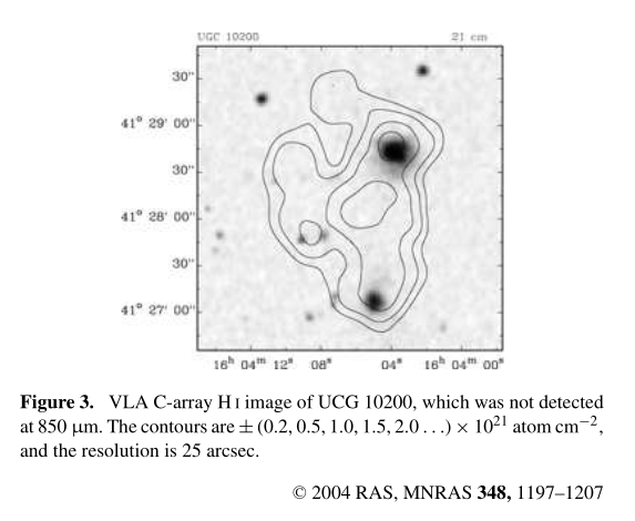
Someday I may undertake a complete census and luminosity function of the cluster system in this galaxy, and perhaps also look at the neighboring starburst galaxy UGC 10200. These systems by the way are cataloged as an interacting dwarf galaxy pair by Paudel et al. (2018) with a total stellar mass of log(M*) = 9.5 and a 3:1 mass ratio, which makes the estimated stellar mass of this galaxy just under 109 M☉. The system is very gas rich, with a neutral hydrogen mass estimated (by the same source) of 109.69 M☉. There are actually at least two published HI maps of this system. The one below, from Thomas et al. (2004) shows that atomic hydrogen extends over essentially the entire extent of the Hubble image above, including the target galaxy.
VLA map of HI gas in UGC 10200 system
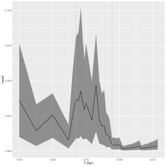
Next I turn to star formation history models for the post starburst spectrum at the top of the post. This uses the same Stan model code as my MaNGA investigations with some minor pre- and post-processing adjustments. I ran two separate models. One used a metal poor subset of the EMILES SSP libraries with Z ∈ {[-2.27], [-1.26], [-0.25]} with, as usual, Kroupa IMF and BaSTI isochrones. I did not attempt to append younger models, so the youngest age is 30Myr. For completeness I also ran a model with my usual EMILES subset + PYPOPSTAR models and Z ∈ {[-0.66], [-0.25], [+0.06], [+0.40]}. First, here is the modeled star formation history with the metal poor subset. I’ve again used a logarithmic time scale and linear star formation rate scale.
Model star formation history of central region of MCG +07-33-040 using metal poor subset of EMILES SSP library
Next is the metal rich subset:
Model star formation history of central region of MCG +07-33-040 using metal rich subset of EMILES+pypopstar SSP library
Both model runs show a fairly steep ramp up in star formation beginning at about 600Myr lookback time and a steep decline around 50Myr ago. The lingering star formation in the metal rich model might be a manifestation of the infamous “age metallicity degeneracy” since Balmer Hα emission is too low to support this level of star formation. Comparing the mass growth histories exposes a more subtle effect: the metal poor models have a consistently higher mass fraction at any given epoch. Also, the period of accelerated star formation involved a slightly smaller fraction of the present day stellar mass.
Mass growth histories of MCG +07-33-040 using metal poor and metal rich subsets of EMILES SSP library
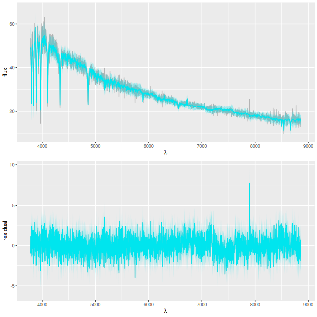
Both models fit the data well. In terms of mean log-likelihood the metal poor model outperformed the metal rich, but only by about 0.4%. The proper Bayesian way to compare models is through the “evidence,” which is hard to estimate accurately. I suspect the metal poor model would be at least slightly flavored because it has fewer parameters than the metal rich one.
Posterior predictive fit to SDSS spectrum of MCG +07-33-040
The duration of accelerated star formation (about which both models agree) is a little surprising in light of simulations that usually show a fairly short SF burst in the first passage in mergers. But, simulations have only explored a small range of the potential parameter range. Studies of low mass galaxies with extended, massive HI haloes might be of interest.
One more sanity check. Suppose the closest approach between our target and UGC 10200 was 60Myr ago, allowing another 10Myr before (presumably) supernova feedback quenched star formation. Assuming the relative motion is transverse to our line of sight traveling 13.2 kpc in 60Myr implies an average separation speed of ≈215 km/sec. This is a perfectly reasonable value for a galaxy pair or loose group.
Finally for this spectrum, here is a quick look at emission line fluxes. Even though visually not at all obvious several lines were detected at marginal (>2σ) to high (>5σ) confidence. A couple of surprises are the [O I] 6300Å line, which is often only marginally detected even in star forming systems, is a firm (3σ) detection and stronger than the usually more prominent [O III] doublet. Also, the [S II] 6717-6730 doublet is a firm detection while the [N II] doublet is not. What this means is unclear to me. Most of the “strong emission line” metallicity indicators that I have formulae for include [N II] (or [O II] which are out of the wavelength range of these spectra), so it isn’t really possible to make a gas metallicity estimate. It’s a safe guess it’s subsolar though.
line
[Ne III] 3869
Hζ
[Ne III] 3970
Hε
Hδ
Hγ
Hβ
[O III] 4959
[O III] 5007
[O I] 6300
[O I] 6363
[N II] 6548
Hα
[N II] 6584
[S II] 6717
[SII] 6730
mean
17.1
2.3
1.5
1.6
1.9
2.1
7.9
2.4
4.9
8.2
2.8
2.9
39.1
2.5
14.4
14.2
s.d.
6.3
2.0
1.4
1.4
1.6
1.8
3.1
2.0
2.9
2.8
1.9
2.0
2.6
1.8
2.8
2.8
ratio
2.7
1.1
1.1
1.1
1.2
1.2
2.6
1.2
1.7
3.0
1.5
1.5
15.2
1.4
5.2
5.2
Flux measurements for tracked emission lines in spectrum of MCG +07-33-040. Units are 10-17 erg/sec/cm2
There are at least two questions about this galaxy that it would be nice to have answers for. First, since the SDSS fiber only includes about 7% of the luminosity and a similar fraction of the stellar mass we really don’t know if it is recently quenched globally or just where SDSS happened to target. My guess from this HST image is that it is globally quenched because its companion UGC 10200 shows clear evidence of dust lanes and extended star forming regions even in this monochromatic image, while the diffuse light in this galaxy looks relatively featureless. A definitive answer would require IFU spectroscopy though.
A second question is whether the star cluster system is truly young or primordial (or both). This would require color measurements from a return visit by HST using at least one more filter in the red. Estimating a luminosity function is feasible with the existing data, although it would have rather shallow coverage. From my casual clicking around the image it appears to be possible to reach magnitudes a little larger than +24 with reasonable precision.
When this topic first came up on the old Galaxy Zoo talk I thought these might comprise a new and overlooked category of galaxies. In fact though all of the examples I investigated belonged to cataloged galaxies and most of the spectra were of small regions in much larger nearby galaxies. A few galaxies that were in the original Virgo Cluster Catalog and excluded from the EVCC because of lack of redshift confirmation should be added back. There were probably only a few like this one with large errors in redshift estimates and high signal to noise spectra. I haven’t spent enough time with the literature to know if rapidly quenched dwarf galaxies are especially interesting. Maybe they are.
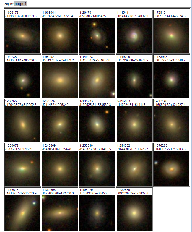
As I mentioned two posts ago there are 24 of these galaxies in the final MaNGA data release, a remarkable 11% of the full sample. I ran my SFH model code on all of these along with the prerequisite redshift offset routine1I actually completed these some time ago. I just haven’t had time to do much analysis or write about them. SDSS thumbnails of the sample are shown below. As expected none of these have significant spiral structure visible at SDSS resolution, but at least a few are noticeably disturbed.
SDSS thumbnail images of Schawinski et al.’s blue early type galaxies in MaNGA final data release (SDSS DR17)
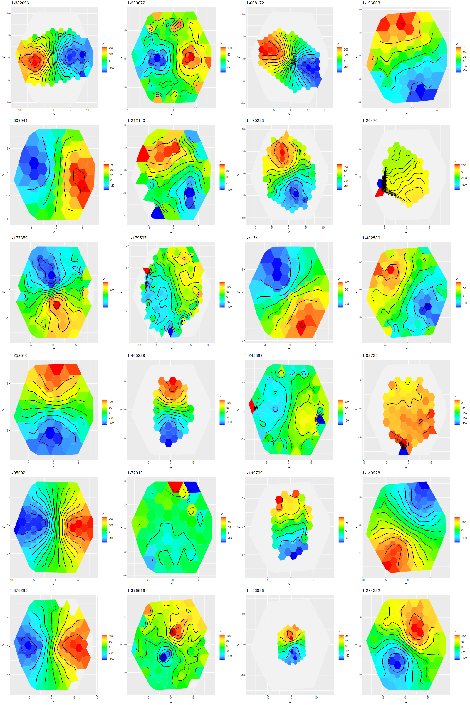
I’m just going to discuss a few topics in this post. I’ll save a more detailed discussion for when I’ve completed analysis of the ancillary post-starburst sample, which is underway now. First, here are velocity fields calculated for the stacked RSS data, with a signal to noise cutoff of 3, the same as I used for my analysis of rotation curves of disk galaxies. Note in the graphic below the ordering is different from the image thumbnails.
Line of sight velocity fields of Schawinski et al.’s blue early type galaxies in the final MaNGA data release
By my count (based entirely on visual inspection) all but 2 of these exhibit large scale rotation, with perhaps 15 or 16 classifiable as regular rotators with the remainder containing multiple velocity components including a couple with (perhaps) kinematically distinct cores. The preponderance of rotating systems surprised me at first, but according to a review by Cappellari (2016) large scale rotation is predominant at least at lower stellar masses (Schawinski et al. characterized their sample as being “low to intermediate mass” among early type galaxies). The velocity fields indicate that many of these contain stellar disks, perhaps embedded in large bulges. That’s still consistent with classification as “early type galaxies.” Apparently the original Galaxy Zoo classification page used the term “elliptical” as the early type galaxy choice, but in the data release paper by Lintott et al. (2011) there’s a statement that the “elliptical” class should comprise ellipticals, S0’s, and perhaps Sa’s from Hubble’s classification scheme.
Depending on how my effort to do non-parametric line of sight velocity modeling goes I may return to examine the kinematics of this sample in more detail, in particular to look for evidence of gas and stellar kinematic decoupling.
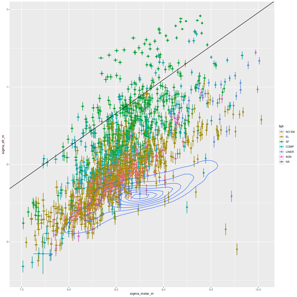
Turning to the recent star formation history this sample runs the gamut from large scale starbursts to passively evolving as seen in the plot of (100 Myr averaged) star formation rate versus stellar mass density for all analyzed binned spectra (of which there were 1525 in the full sample). For reference the straight line is my estimate of the center of the local “spatially resolved star formation main sequence.” This is just a weighted least squares fit to the sample of 20 non-barred spirals with star forming BPT diagnostics that I discussed some time ago. My SFMS relation has the same slope as estimated by Bluck but is offset higher by about 0.7 dex, which probably just reflects the very different methods used to estimate star formation rates. The contour lines are the densest part of the relationship from the passively evolving Coma cluster sample that I also discussed in that post. The majority of the blue etg sample falls in the green valley, consistent with Schawinski et al.’s observation that only about 1/2 of the sample showed evidence for ongoing star formation.
“Spatially resolved” star formation rate density versus stellar mass density for 24 blue early type galaxies in final MaNGA data release. Contour lines are corresponding values for 33 passively evolving Coma cluster galaxies.
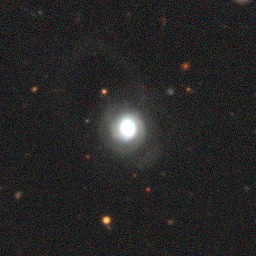
Most of the points offset the most on the high side of the SFMS come from just two galaxies: MRK 888, which I’ve discussed in the last few posts, and SDSS J014143.18+134032.8 (this is apparently not in any “classical” catalog). The legacy survey cutout below clearly shows an extended tidal tail that’s a certain sign of a relatively recent merger.
SDSS J014143.18+134032.8, a disturbed, star-bursting blue early type galaxy
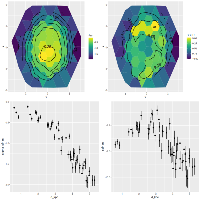
I just want to take a quick look at this one: below are maps of the star formation rate density and SSFR as well as scatterplots of the same against distance from the IFU center. As with MRK 888 ongoing star formation is widespread with a peak near the center, a classic case of a merger fueled starburst. In this galaxy star formation peaks in a ring somewhat outside the nucleus. The ring can be seen clearly in the SDSS cutout and must consist of HII regions.
SDSS J014143.18+134032.8 (mangaid 1-41541; plateifu 8095-1902)
Star formation rate density and specific star formation rate – maps and scatterplots against radius in kpc.
Schawinski et al. briefly discuss the possibility that their blue ETG’s could be progenitors of E+A (aka K+A) galaxies. This galaxy and MRK 888 are plausible candidates — if star formation shut off rapidly they would certainly exhibit strong Balmer absorption for a time after emission lines disappeared since they already do. Other members of this sample are already fading towards the red sequence, and if they ever qualified as “post-starburst” it must have been in the past.
I plan to look at star formation histories in more detail after I’ve completed model runs on the MaNGA post-starburst sample.
This is still experimental and I’m not sure how much farther I’ll pursue it, but I tried a straightforward way to add emission lines to non-parametric line of sight velocity distribution (LOSVD) models. The idea is simple enough: model the line profiles directly using Stan’s simplex data type with each modeled line represented by a vector of mostly zeroes and with the simplex centered on the line’s rest wavelength. Although not essential I’m assuming I will have estimates of redshift offsets for each fiber or spaxel in a MaNGA data file (RSS or cube), so any additional offsets should be small. I’ve chosen to ignore the fact that the discretized line profiles will differ between lines because their central wavelengths will fall at different points within their assigned wavelength bins. Also, different lines could arise from kinematically distinct regions, which is not uncommon in galaxies with broad line AGNs. The obvious solution to this is to allow multiple line profiles. For these initial exercises I’m using a single line profile for all modeled lines (I fit 18 at present). As I’ve done since I started these modeling exercises I am fitting emission lines and stellar contributions simultaneously, with the stellar part represented by a small set of eigenspectra derived from my usual EMILES based library.
Below the “fold” I’ve included the Stan code in it’s current (but certainly not final) form. About half of the code for modeling the stellar LOSVD, is adopted from the original version that I wrote about last year. The emission line model portion takes advantage of an odd feature of Stan, namely the ability to store a matrix in sparse form and perform one specific operation — matrix multiplication with a vector. I still haven’t figured out the particular matrix representation used, so I just create a dummy matrix for the emission lines in the transformed data section and extract the two vectors describing the positions of the non-zero elements of the matrix. In the model section the simplex vector representing the line profiles is repeated as many times as there are lines to fill in the non-zeros.
Another thing to note is that Stan doesn’t know how to work with missing data. In general there will be gaps in spectra that were masked for some reason, while the input templates must be complete over the covered spectrum (plus a few extra at each end for the convolution). This requires a bit of housekeeping that’s mostly done in the R code that sets up the input data.
In the models I ran last year I ignored dust reddening since I didn’t expect it to be significant in the passively evolving Coma cluster galaxies I tested them on. In general reddening isn’t ignorable though and there’s the potential for template mismatch without some allowance for it. For now I inserted the function I use for “modified Calzetti” attenuation but it’s not actually used. In the one test I tried including attenuation in the model significantly increased execution time. I will probably look at using a multiplicative polynomial for the same purpose. A final thing to note is there are no explicit priors for the two simplex vectors that represent the stellar velocity convolution kernel and emission line profile, which means that the priors default to a maximally diffuse dirichlet distribution. This turns out to be an important issue that I will discuss further below.
I’ve run sets of models for a small sample of galaxies so far. so lets look at some results. For these runs I used 500 warmup and 500 post-warmup iterations per chain with 4 parallel chains for a total post-warmup sample size of 2000. The stellar templates are represented by 6 eigenspectra created from singular value decompositions of my standard EMILES based SSP library. I currently fit 18 emission lines — Balmer lines from Hα through Hζ and a selection of the stronger forbidden lines. Model runs typically take 2-3 minutes for sampling on my old 4th generation Intel core I7 based PC. This can undoubtedly be reduced by factors of at least several with multithreading.
In this post I’m going to look in some detail at results for Markarian 888, which was the main topic of my last post. Recall this is one of Schawinski’s “blue early type galaxies” that turns out to have obvious spiral-like structure in its inner region and clear evidence for a relatively recent merger.
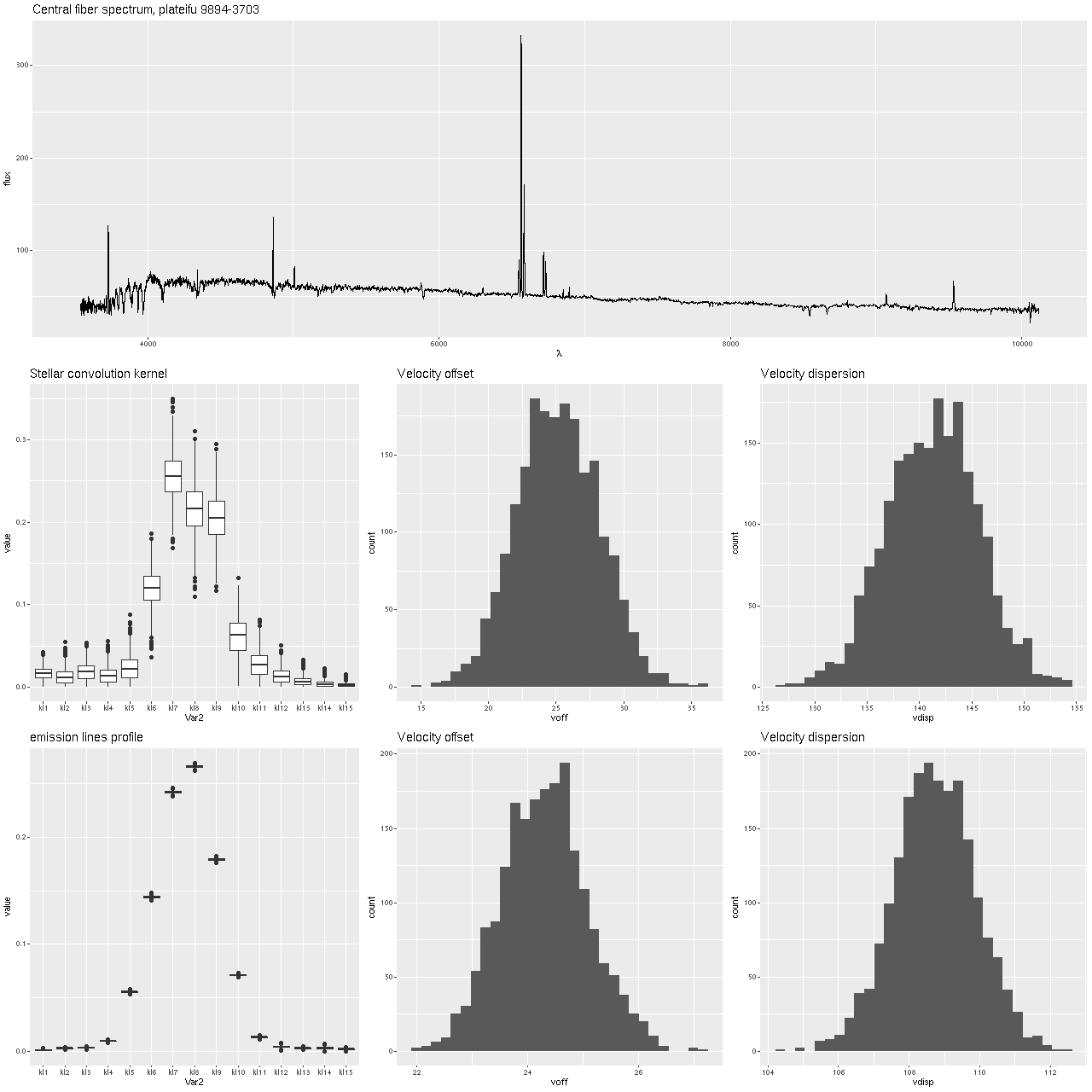
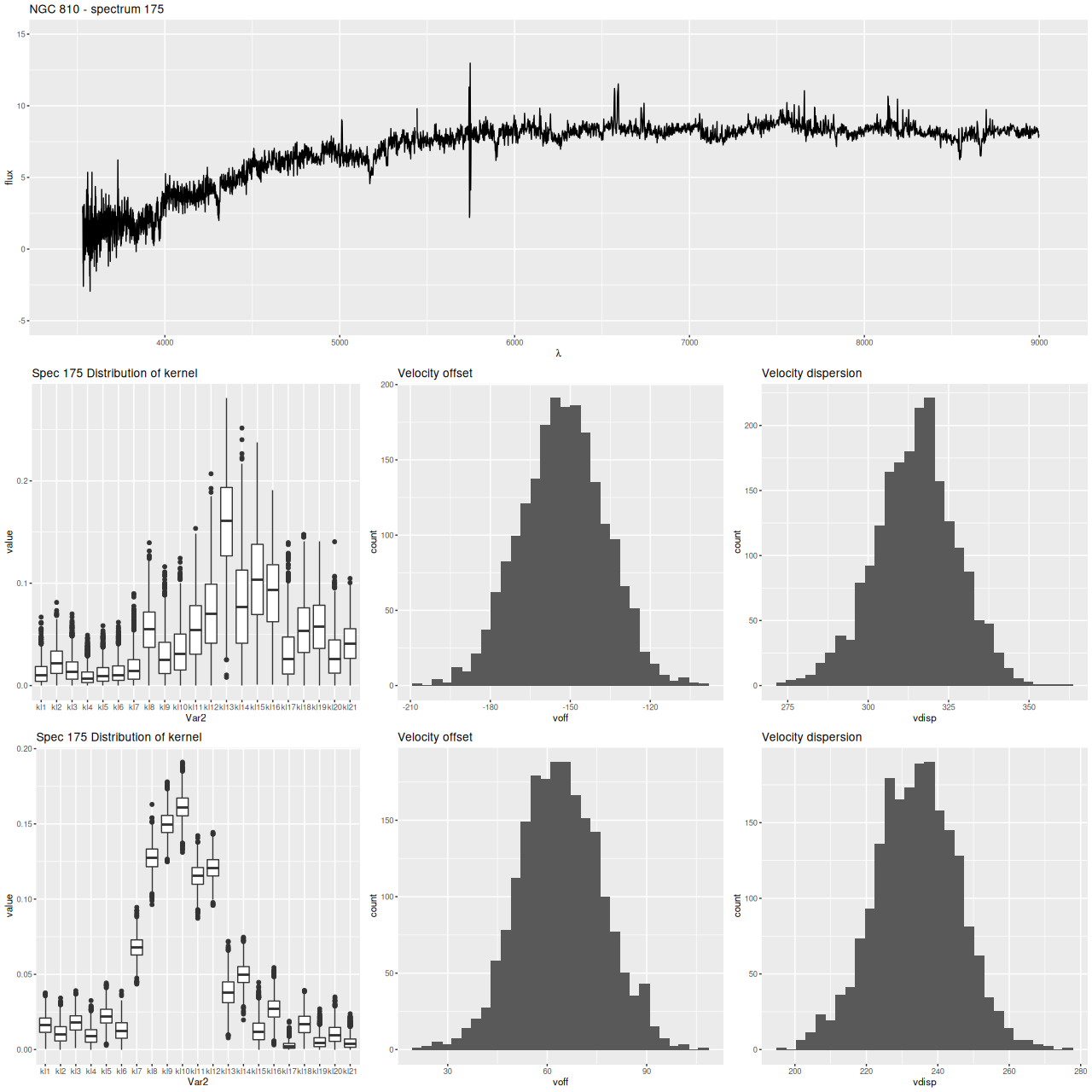
First, the graph below shows the central fiber spectrum, and below that the results of a model run for the stellar velocity convolution kernel. From those I can calculate velocity offsets1these formulas are approximate but close enough for the present purpose.
\(
\delta v = 69 \times \sum\limits_{k = -\lfloor K/2 \rfloor}^{\lfloor K/2 \rfloor} k p_i
\)
for each draw from the posteriors, and these are shown as histograms in the middle and right graphs. This was a high signal to noise spectrum with prominent emission and absorption lines, a favorable situation for this modeling exercise and in fact the results look very promising with an especially well determined distribution for the emission lines. In summary, the posterior mean stellar velocity offset was 25 km/sec. with a 95% credible interval of (19.8, 31.3), while the corresponding values for emission lines were 24.3 and (22.8, 25.9), so the credible interval for emission lines lies entirely within that for stars.
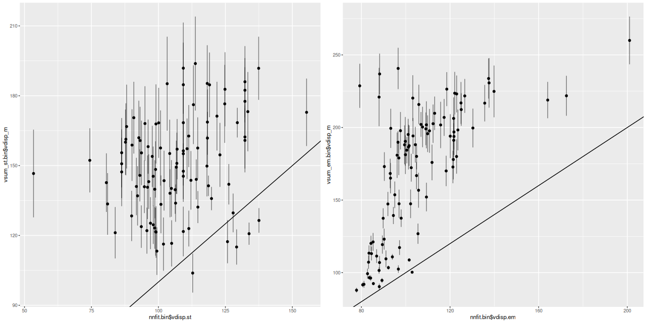
The corresponding values for velocity dispersions on the other hand differ quite a lot: 141 km/sec. for stars with a 95% credible interval of (133.6, 150.3) versus 109 km/sec and (106, 111) for gas. I’ll say some more about this below, but I think this is already a sign that the second moments (at least) of these velocity distributions need to be treated with caution.
Markarian 888 – mangaid 9894-3703
Central fiber spectrum, modeled stellar and ionized gas losvd
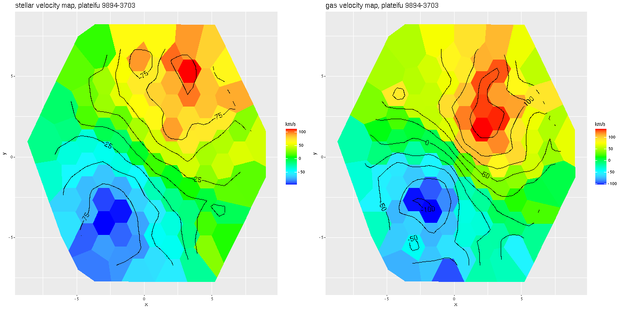
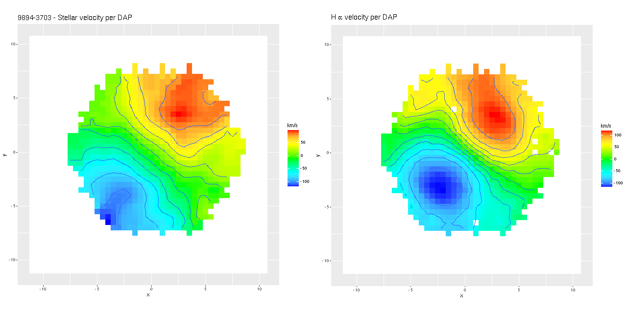
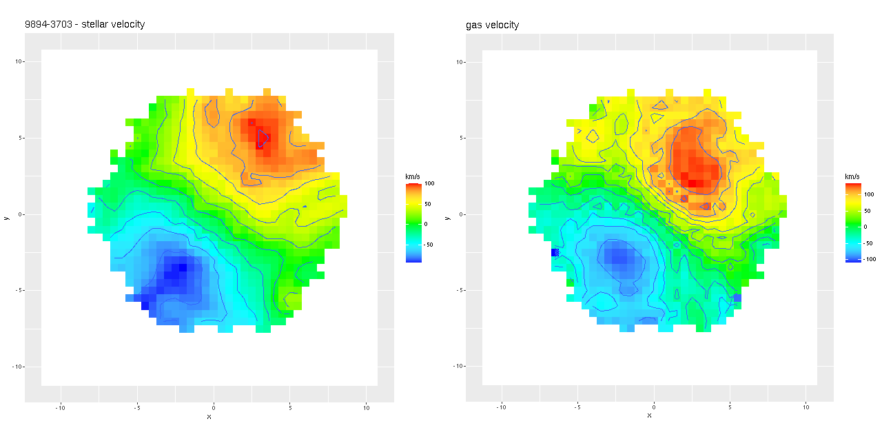
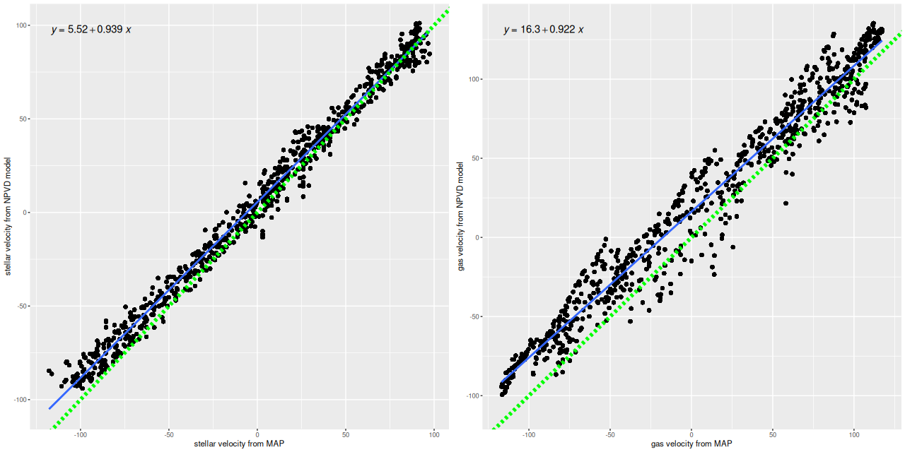
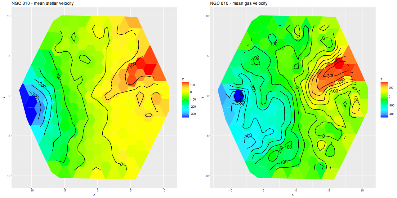
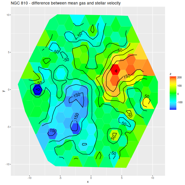
After running the code for every binned spectrum in the IFU I get stellar and gas velocity maps as shown below. These look similar to each other and to the map in the last post based on my hybrid red shift offset fitting routine, although a closer look will show a systematic decoupling of gas and stellar velocities.
Stellar and ionized gas velocity maps for Mrk 888 (MaNGA plateifu 9894-3703)
I often take a look at the official MaNGA data analysis pipeline results, usually through the “Marvin” interface. Generally my results look similar for any given quantity, but it’s hard to tell how closely since we’re looking at different things (binned RSS spectra vs. cubes, for one) and I’m really just doing a visual comparison. As more or less a one off exercise I decided to compare velocity fields from the cubes. First, here are stellar and Hα maps from the DAP. These are from the “HYB10-MILESHC-MASTARSSP” sequence, which refers to the binning strategy and template inputs.
Mrk 888 – stellar and gas velocity fields derived from non-parametric LOSVD models
Next are my stellar and ionized gas velocity maps. Evidently these are considerably “noisier” in appearance, but similar overall. The noisiness may be due to different binning strategies: I modeled velocity distributions for every spaxel that met a minimal signal to noise requirement.
Mrk 888 – stellar and gas velocity fields derived from non-parametric LOSVD models
For a more quantitative comparison here are scatterplots of the mean stellar and gas velocity offsets from my runs against the MaNGA DAP. Both of these show slight tilts, that is the slopes are less than one, and small offsets. I’m tempted to suspect systematic errors somewhere, but I haven’t found any yet. And I have no hypothesis about the decidedly non-random behavior of the gas velocity plots. So there are still questions to be answered, but the magnitude of differences is no more than about ±1 wavelength bin (69 km/sec). For my main purposes this is good enough.
Mrk 888 – scatter plot of mean stellar and gas velocities – my models vs. DAP
One more pair of graphs for this galaxy. In the initial maximum likelihood fit to a spectrum I estimate stellar and gas velocity dispersions with a single component gaussian. The graphs below plot the velocity dispersions from the Bayesian models calculated by the formula above against the ML fit values. The stellar velocity dispersions behave pretty much the same as I noted before: there’s a weak positive correlation between the non-parametric models and the maximum likelihood estimates with the former generally offset to higher values. The gas velocity dispersion estimates show an even larger discrepancy along with an apparently nonlinear trend.
Mrk 888 – velocity dispersions from Bayesian nonparametric losvd models vs. estimates from maximum likelihood fitting
More briefly now, since this got longer than I wanted. I also ran models for the “Zoogems” target NGC 810, which I noted two posts ago has interesting kinematics, in particular a rapidly rotating disk that isn’t evident in the stellar velocity map from the DAP. From the maps below we see that the rapidly rotating component is the ionized gas, which has a mean rotation velocity as much as 150 km/sec larger than the stellar component.
NGC 810 – mean stellar and gas velocity mapsNGC 810 – difference between mean gas and stellar velocities
Finally, here are two more graphs of the kinematic models for the spectra with the largest positive and negative differences between stellar and gas velocity (these are the reddest and bluest patches in the map above. These show the spectra in the top row, followed by the posterior distribution of the stellar LOSVD and distributions of the first two moments, then the same for the emission line profiles.
NGC 810 – sample MaNGA spectrum, non-parametric stellar LOSVD and emission line profileNGC 810 – sample MaNGA spectrum, non-parametric stellar LOSVD and emission line profile
The second set of graphs illustrates a significant problem: when there’s poor data — in this case no detectable emission lines — the models tend to return the prior, which for now is a maximally diffuse dirichlet. This will bias second moment estimates to the high side and can lead to spurious correlations, for example the increase of velocity dispersion with radius that I noted in the last post on this topic.
At the same time this spectrum is in the region of overlap between the main galaxy and its companion, and two peaks in the stellar velocity distribution are clearly seen at about the right velocity offset (~340 km/sec).
A short to do list:
Investigate informative priors.
Allow for dust reddening. I tried using a modified Calzetti attenuation relation in the code (note its presence in the code below, although it’s not used in the model), but it adds too much to execution time. A low order multiplicative polynomial might suffice.
Investigate systematics between my estimates and those in the DAP.