I’m going to end this series for now with a more detailed look at the spatially resolved star formation history of this galaxy and make a highly selective comparison to some recent theoretical and empirical work on mergers. This continues from part 1 and part 2.
My main theoretical sources for the following discussion include a paper titled “The fate of the Antennae galaxies” by Lahén et al. (2018) and a similar paper also simulating an Antennae analog by Renaud, Bournaud and Duc (2015). I didn’t pick these because I necessarily think this galaxy is an evolved analog of the Antennae; in fact I think there are important differences in the likely precursors. The main reason is these studies are among the first to run very high resolution simulations through and beyond coalescence. Some other significant papers include high resolution simulations with detailed treatment of feedback by Hopkins et al. (2013), Di Matteo et al. (2008), who studied a large sample of merger and flyby simulations, Bekki et al. (2005) who specifically looked at the formation of K+A galaxies through mergers, and Ji et al. (2014) who studied the lifetime of merger features using a suite of simulations. This doesn’t begin to scratch the surface of this literature. Merger simulations are very popular!
Some recent observational papers that examine individual post-merger systems in more or less detail include Weaver et al. (2018) and Li et al. (2018). I will return to the latter paper, which was based on MaNGA data, in a later post. Other observational work that’s more statistical in nature includes Ellison et al. (2015), Ellison et al. (2013), and earlier papers in the same series.
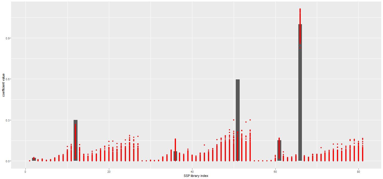
As I’ve mentioned several times already the model spectra I use mostly come from the 2017 EMILES extension of the MILES SSP library with BaSTI isochrones and Kroupa IMF, supplemented with unevolved model spectra from the 2013 update of BC03 models. The results reported in the previous two posts used a small subset of the library — just 3 metallicity bins and 27 time bins, with every other time bin in the full library starting with the second excluded. For my “full” MILES subset I use 4 metallicity bins with \([Z/Z_{\odot}] \in \{-0.66, -0.25, 0.06, 0.40\}\) and all 54 time bins (the lowest metallicity bin is dropped in the reduced subset). Execution time of the Stan SFH models is roughly proportional to the number of parameters, so everything else equal it takes about 2.5 times longer to run a single model with the full set.
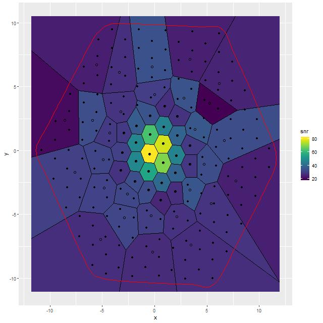
For this exercise I binned the MaNGA spectra with a considerably higher target SNR than usual, ending up with 53 coadded spectra out of the original 183 fiber/pointing combinations. One of the mods I made to Cappellari’s Voronoi binning code was to drop a “roundness” check. The bins in this case still end up with reasonably compact shapes since the surface brightness within the IFU footprint is fairly symmetrical. All but one of the spectra in the inner 2 kpc. ended up unbinned, so the spatial resolution in that critical region is unchanged.
To directly compare the results from the current round of models with the previous lower time resolution runs here are the modeled mass growth histories summed over the entire IFU footprint (blue is the EMILES subset):
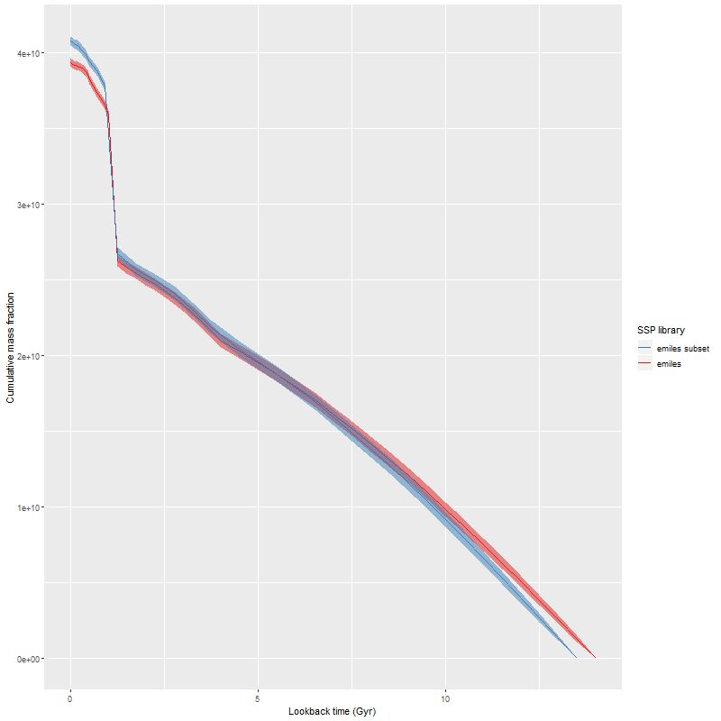
Note: MaNGA’s dithering strategy results in considerable overlap in fiber positions in order to obtain a 100% filling fraction. That means the area in fibers exceeds the area of the IFU footprint by about 60%. So, sums of quantities like masses or star formation rates need to be adjusted downwards by about 0.2 dex.
The only real difference we see in the higher time resolution runs is that the initial, strongest starburst is a few percent weaker, and there are some subtle differences in late time behavior. The first large starburst begins at 1.25 Gyr in both sets of runs, and unfortunately this bin is 250 Myr in width in the full resolution set, vs 350 Myr in the subset, so we don’t really get significantly finer grained estimates of the SFH in the initial burst.
We can get a rough idea of the nature of the precursors from this graph. The present day stellar mass is \(4 \times 10^{10} M_{\odot}\), of which just about a third was formed in or after the initial starburst. The present day combined stellar mass of the precursors was just over \(2.6 \times 10^{10} M_{\odot}\) just before the burst — the then stellar mass would have been somewhat larger since this mass growth estimate includes mass loss to stellar evolution. Also, there’s considerable light and therefore stellar mass outside the IFU footprint — the drpcat value for the effective radius is 5.5″ while the Petrosian radius per the SDSS photo pipeline is 12.5″. The IFU footprint is about 10″ radius, or about 1.8 effective radii. Taking a guess that we’re sampling about 80% of the stellar mass the values above need to be adjusted upwards by 25%. Assuming the precursors were equal mass and rounding up their pre-merger stellar masses would be around \(1.65 \times 10^{10} M_{\odot}\). Guessing the current total stellar mass to be \(5 \times 10^{10} M_{\odot}\) then \(1.7 \times 10^{10} M_{\odot}\) was added by the merger. The amount of gas turned into stars was actually higher — about \(2.4 \times 10^{10} M_{\odot}\), but some, maybe most, of the gas lost to stellar evolution might have been recycled. But, I’ll be conservative and adopt the higher value. If that was divided equally between the progenitors they would have had gas masses around \(1.2 \times 10^{10} M_{\odot}\) just before the merger, or just over 40% of the baryonic mass. While high that’s not extraordinarily so for a late type spiral in that stellar mass range (see for example Ellison et al. 2015, figures 6-7).
These values are rather different from the putative Antennae analogs in the two studies linked above, which are in turn rather different from each other. Lahén et al. assign equal stellar masses of \(4.7 \times 10^{10} M_{\odot}\) to each progenitor, equal gas masses of \(0.8 \times 10^{10} M_{\odot}\) (14.5% of the total baryonic mass), and a baryonic to total mass ratio of 0.1. The simulations of Reynaud et al. have stellar masses of \(6.5 \times 10^{10} M_{\odot}\) apiece, gas masses of just \(0.65 ~\mathrm{and}~ 0.5 \times 10^{10} M_{\odot}\), and dark matter halos of \(23.8 \times 10^{10} M_{\odot}\) (for a baryonic to total mass ratio of about 23%). The merger timescales are rather different too: 180 Myr from first pericenter passage to coalescence for the Reynaud et al. simulations vs. ~600 Myr for Lahén et al. (the latter seems closer to the observational evidence; for example Whitmore et al. 1999 found clusters with 3 distinct age ranges up to ~500Myr, with the oldest argued to have formed in the first pericenter passage).
The qualitative features of the merger progress are similar however, and some are fairly generically observed in simulations. There are two pericenter passages, with a second period of separation followed shortly by coalescence at the third pericenter. Star formation is widespread but clumpy in the first flyby, with a large but short starburst and slow decline. A stronger, shorter, and more centrally concentrated starburst occurs around the time of the second pericenter passage through coalescence. The Lahén simulations follow the merger remnant for another Gyr — they show an exponentially declining SFR from an elevated level immediately after coalescence. Neither of these sets of simulations attempt to model AGN feedback, which would presumably cause more rapid quenching. Notably, the Lahén merger remnant develops a kinematically decoupled core although overall the remnant is a fast rotator. Unless the rotation axis is pointing right at us this galaxy is a slow rotator except for the core.
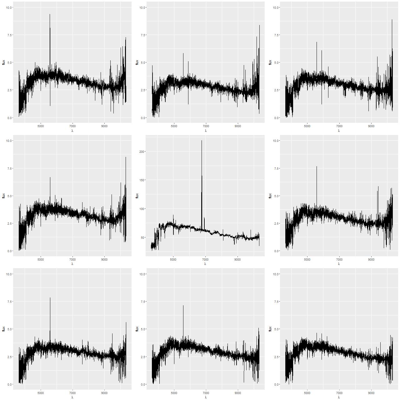
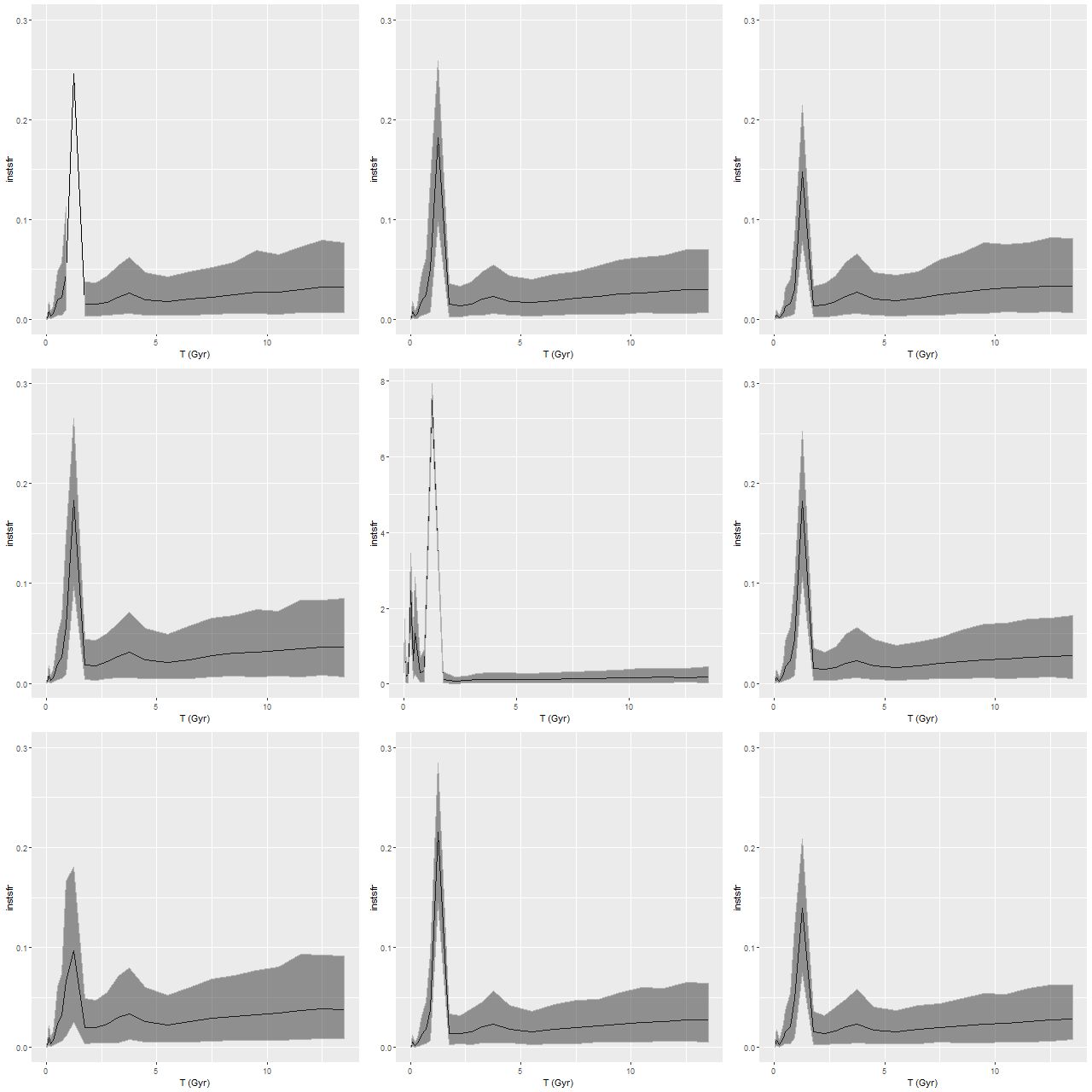
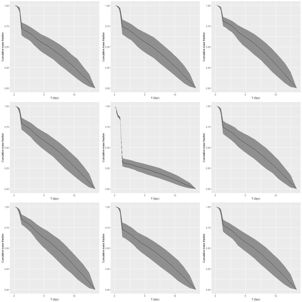
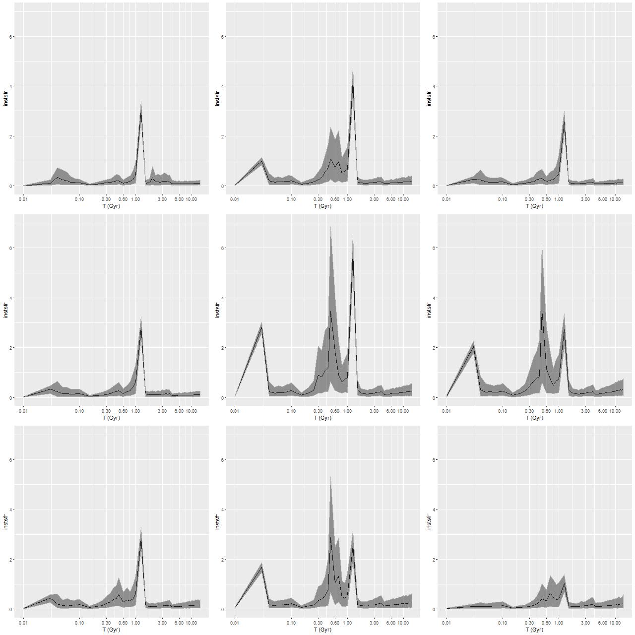
Getting back to data for this galaxy I show some star formation history plots below, first for the inner 9 fibers (all within <1.25 kpc of the nucleus). Below that are a pair of plots of aggregate SFH for fibers within 2.5 kpc (left) of the nucleus and outside that radius (right). The time axis on these plots is logarithmic since I want to focus on the late time behavior (and also this is closer to the real time resolution). Note that in the inner region there are 3 broad peaks in star formation rate — the previously discussed one at 1-1.25Gyr, one centered around 500Myr, and a recent (\(\lesssim\)100Myr revival that peaks at the youngest BaSTI age of 30Myr. The relative and absolute sizes of the peaks are highly variable, indicating that the stars aren’t fully relaxed yet. The outer region covered by the IFU by contrast has just a single peak at 1-1.25Gyr, with a more or less monotonic decline thereafter.
If we believe the models the straightforward interpretation is the first pericenter passage happened about 1-1.25Gyr ago, with coalescence around 500Myr ago and continued infall or recycling driving the ongoing star formation. This is consistent with simulations, which can have merger timescales ranging anywhere from a few hundred Myr to several Gyr. The main problem with this interpretation is that in most simulations the highest peak SFR occurs around coalescence, with the integrated SF roughly equally divided between the first passage and during/after coalescence. In these models about 75% of the post-burst star formation occurs in the 1-1.25Gyr bin, with about 23% in the later burst. An alternative scenario then would be that the entire merger sequence occurred in the 250Myr window of the 1-1.25Gyr bin, and everything since is due to post-merger infall. Of course a third possibility, which I don’t dismiss, is that the details of the modeled episodes of star formation are just artifacts having no particular relationship to the real recent star formation history. The main argument I have against that is that all the spectra seem to tell a consistent story of multiple recent episodes of star formation of varying strength in space and time, and with clear radial trends.
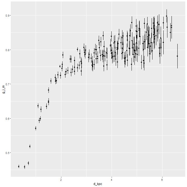
Regardless of the details this galaxy nicely confirms several of the predictions of Bekki et al. (linked above). As we saw in the last post there is a positive color gradient and negative Balmer absorption gradient as they predict for dissipative major mergers, with a break in the color gradient trend that corresponds approximately with the boundary between multi-peaked and single peaked late time star formation histories.
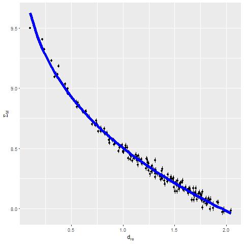
The obvious morphological indicators of disturbance are provocative but don’t seem to be highly constraining. My recollection is that folklore guesstimates that tidal features have a visible lifetime of ~1 Gyr. Ji et al. (linked above) on the other hand found based on a suite of simulations that merger features remain visible at the 25 mag./arcsec\(^2\) somewhat longer, on average about 1.4Gyr. It may be significant that the disturbance is easily seen even in the SDSS Navigate imaging, especially the northern loop. The somewhat similar star forming elliptical SDSS J1420555.01+400715.7 discussed by Li et al. (which I will turn to later) required deeper imaging and some enhancement to show signs of disturbance. One thing I’m working on learning is galaxy profile fitting and photometric decomposition. I’d like to see if the single component Sersic fit that fit the mass density profile also works for the surface brightness (I suspect there is a steeper core). I’d also like to quantify the surface brightness in the tidal features. These are exercises for later.
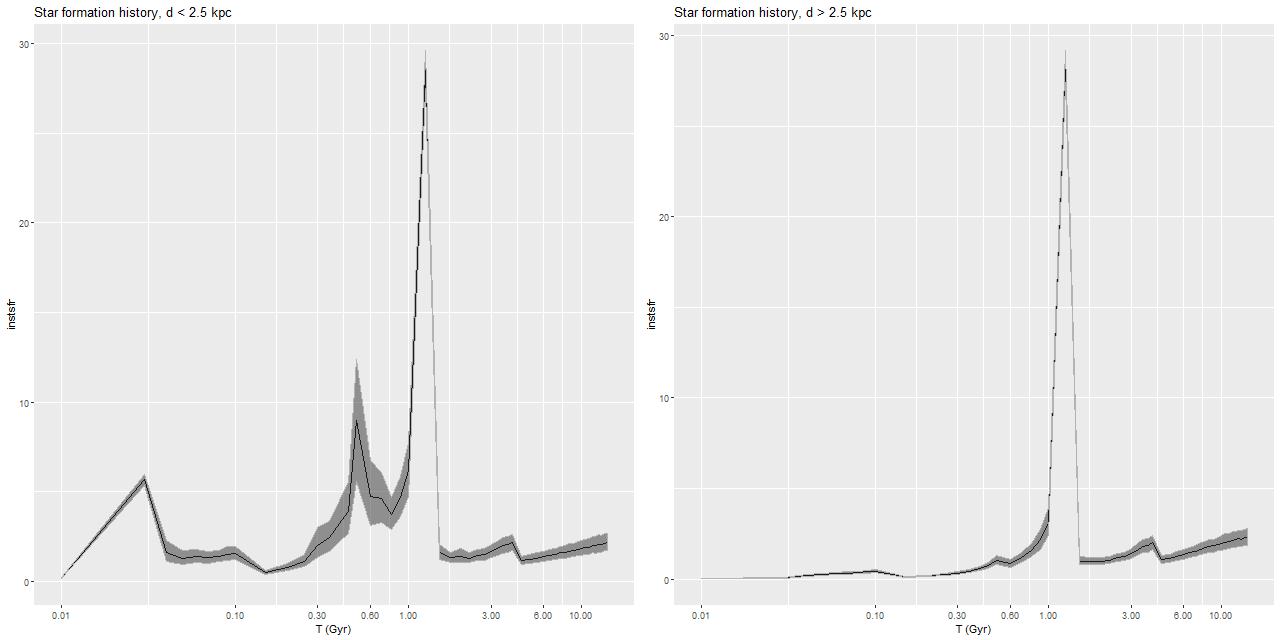
L – d ≤ 2.5 kpc
R – d > 2.5 kpc
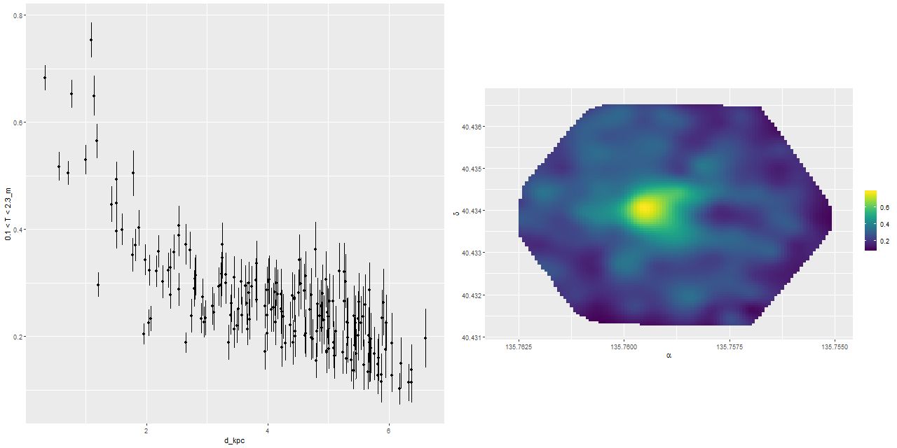
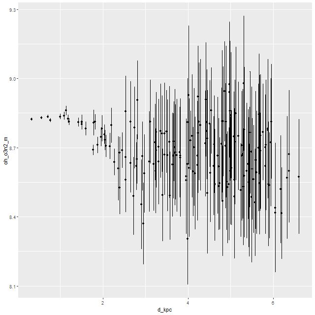
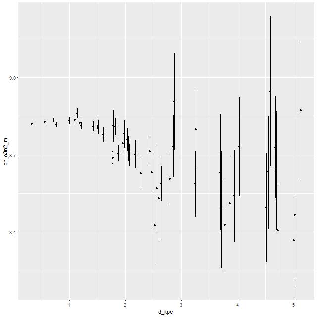
I’m going to conclude with a few plots of quantities that I thought might benefit from the higher S/N in the binned spectra. First is the gas phase metallicity from the O3N2 index plotted against radius. Unfortunately emission line strengths are still too weak beyond about 2.5 kpc radius to say much about the outskirts, but we still see a fairly flat trend with radius up to ~1.5 kpc with a turnover to lower values that continues at least out to ~2.5kpc. This is broadly similar with the simulations of Lahén et al., who obtained a shallower metallicity gradient for their merger remnant than an undisturbed spiral galaxy.
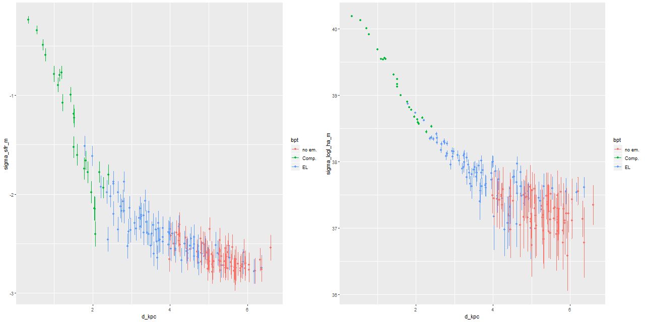
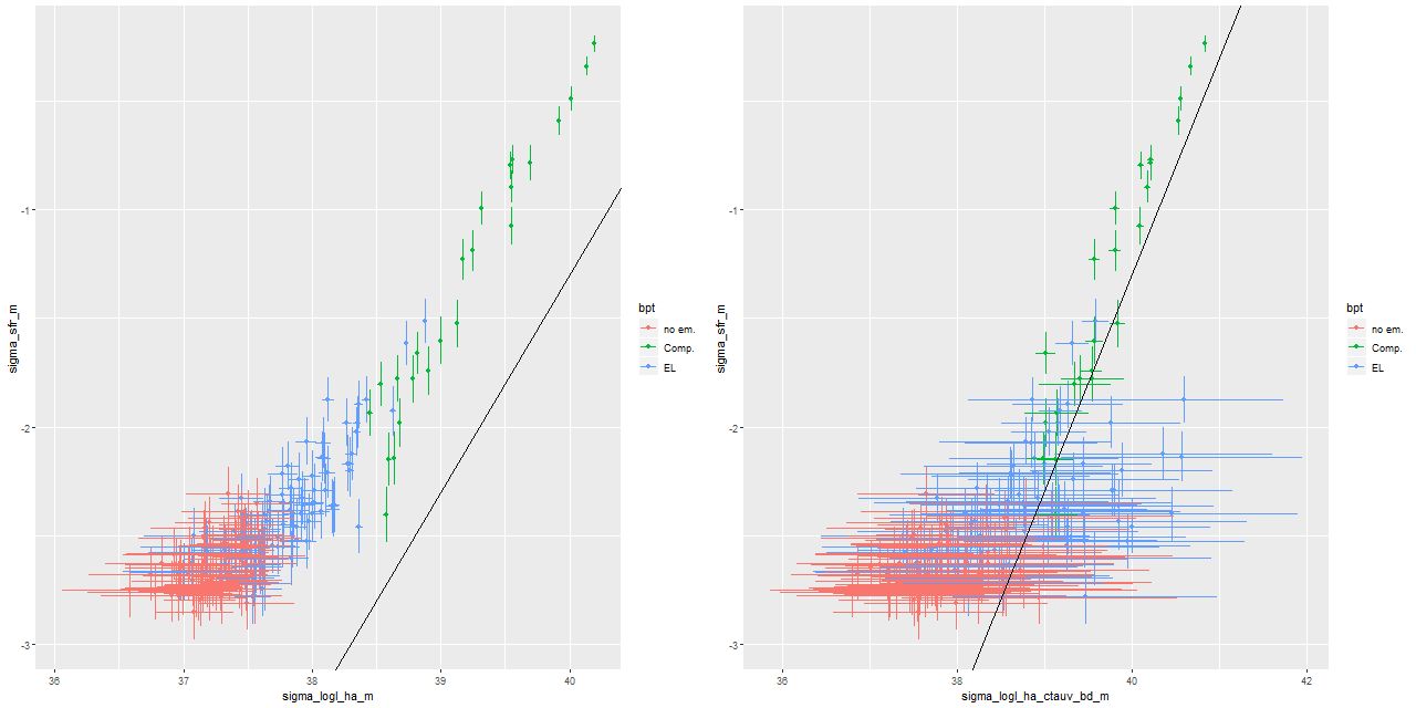
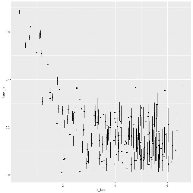
Here I again plot the estimated SFR density against radius and the estimated SFR density against Hα luminosity density. The high luminosity end is essentially unchanged from the plot in the last post since these spectra are unbinned. Again, the points at the high luminosity end lie above the Hα-SFR calibration of Moustakas et al. by considerably more than the nominal length of the error bars, which points to a likely recent (< ~10Myr) fading of star formation. This is consistent with the detailed SFH models. At the other end of the luminosity scale there seems to be an excess of points to the right of the calibration line. This could indicate that the main ionization source in the outer regions of the IFU footprint is something other than massive young stars (presumably shocks or hot evolved stars).
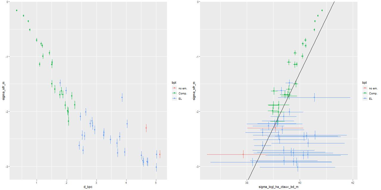
R – SFR density vs. Hα luminosity density
Binned spectra with enlarged EMILES SSP library
Despite the “composite” emission line ratios in the central region there’s little evidence for an AGN. The galaxy is a compact FIRST radio source, but the size of the starforming region is right around the FIRST resolution. The raw WISE colors are W1-W2 = +0.07, W2-W3 = +2.956, which is well within the locus of spiral colors.