A little more on Schawinski’s blue early type galaxies

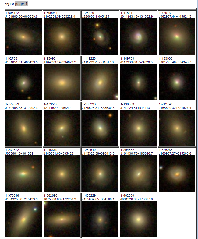
As I mentioned two posts ago there are 24 of these galaxies in the final MaNGA data release, a remarkable 11% of the full sample. I ran my SFH model code on all of these along with the prerequisite redshift offset routine1I actually completed these some time ago. I just haven’t had time to do much analysis or write about them. SDSS thumbnails of the sample are shown below. As expected none of these have significant spiral structure visible at SDSS resolution, but at least a few are noticeably disturbed.

thumbnails_blueetg
SDSS thumbnail images of Schawinski et al.’s blue early type galaxies in MaNGA final data release (SDSS DR17)

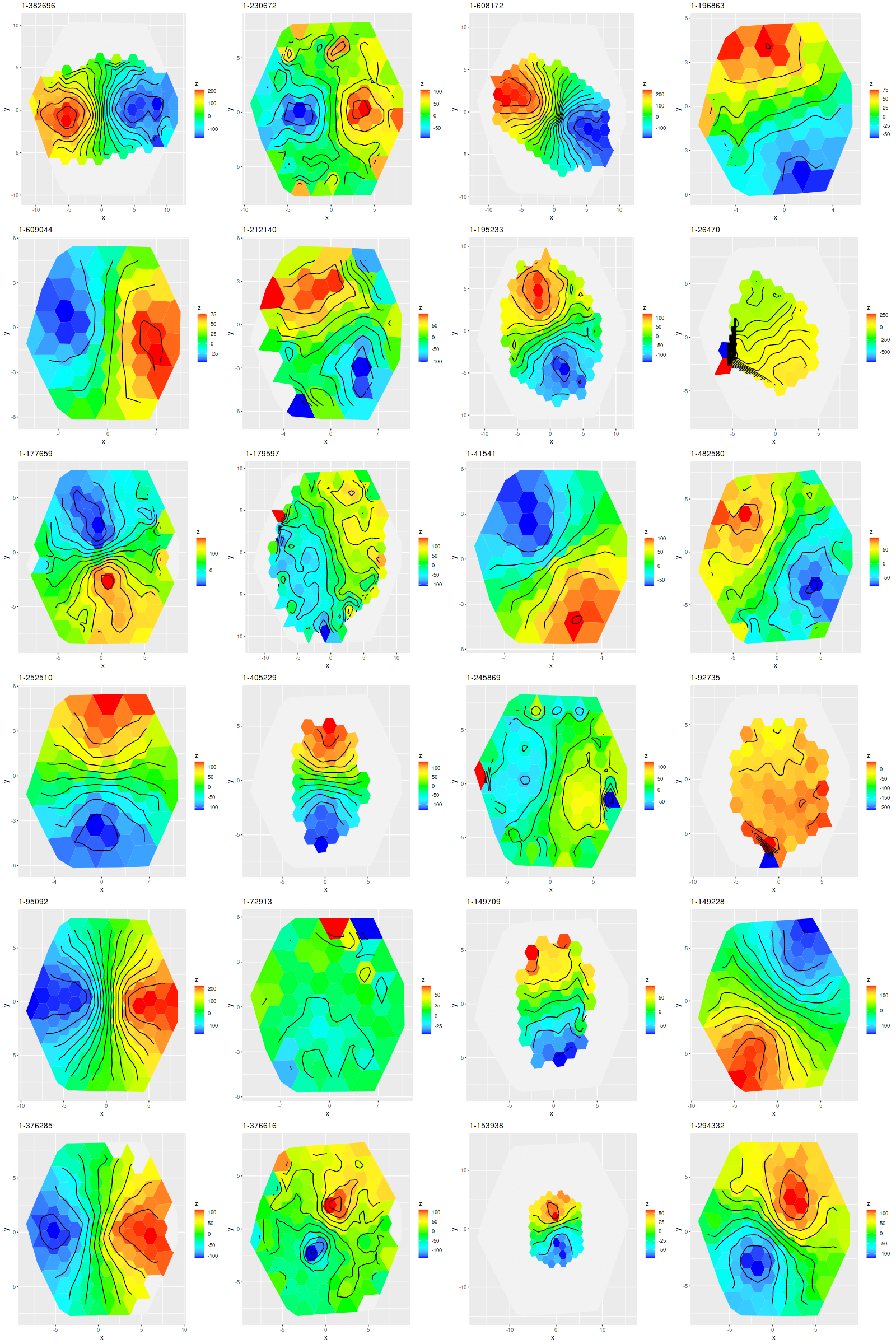
I’m just going to discuss a few topics in this post. I’ll save a more detailed discussion for when I’ve completed analysis of the ancillary post-starburst sample, which is underway now. First, here are velocity fields calculated for the stacked RSS data, with a signal to noise cutoff of 3, the same as I used for my analysis of rotation curves of disk galaxies. Note in the graphic below the ordering is different from the image thumbnails.

vfs_blueetg
Line of sight velocity fields of Schawinski et al.’s blue early type galaxies in the final MaNGA data release

By my count (based entirely on visual inspection) all but 2 of these exhibit large scale rotation, with perhaps 15 or 16 classifiable as regular rotators with the remainder containing multiple velocity components including a couple with (perhaps) kinematically distinct cores. The preponderance of rotating systems surprised me at first, but according to a review by Cappellari (2016) large scale rotation is predominant at least at lower stellar masses (Schawinski et al. characterized their sample as being “low to intermediate mass” among early type galaxies). The velocity fields indicate that many of these contain stellar disks, perhaps embedded in large bulges. That’s still consistent with classification as “early type galaxies.” Apparently the original Galaxy Zoo classification page used the term “elliptical” as the early type galaxy choice, but in the data release paper by Lintott et al. (2011) there’s a statement that the “elliptical” class should comprise ellipticals, S0’s, and perhaps Sa’s from Hubble’s classification scheme.

Depending on how my effort to do non-parametric line of sight velocity modeling goes I may return to examine the kinematics of this sample in more detail, in particular to look for evidence of gas and stellar kinematic decoupling.

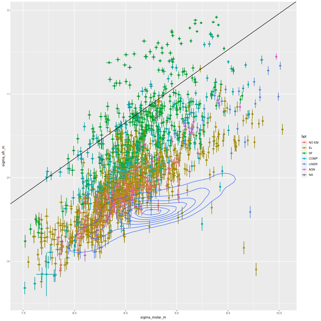
Turning to the recent star formation history this sample runs the gamut from large scale starbursts to passively evolving as seen in the plot of (100 Myr averaged) star formation rate versus stellar mass density for all analyzed binned spectra (of which there were 1525 in the full sample). For reference the straight line is my estimate of the center of the local “spatially resolved star formation main sequence.” This is just a weighted least squares fit to the sample of 20 non-barred spirals with star forming BPT diagnostics that I discussed some time ago. My SFMS relation has the same slope as estimated by Bluck but is offset higher by about 0.7 dex, which probably just reflects the very different methods used to estimate star formation rates. The contour lines are the densest part of the relationship from the passively evolving Coma cluster sample that I also discussed in that post. The majority of the blue etg sample falls in the green valley, consistent with Schawinski et al.’s observation that only about 1/2 of the sample showed evidence for ongoing star formation.

sfr_mstar_blueetg
“Spatially resolved” star formation rate density versus stellar mass density for 24 blue early type galaxies in final MaNGA data release. Contour lines are corresponding values for 33 passively evolving Coma cluster galaxies.

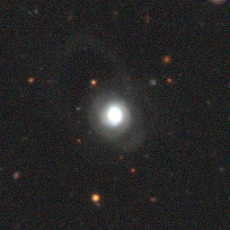
Most of the points offset the most on the high side of the SFMS come from just two galaxies: MRK 888, which I’ve discussed in the last few posts, and SDSS J014143.18+134032.8 (this is apparently not in any “classical” catalog). The legacy survey cutout below clearly shows an extended tidal tail that’s a certain sign of a relatively recent merger.

SDSS J014143.18+134032.8, a disturbed, star-bursting blue early type galaxy

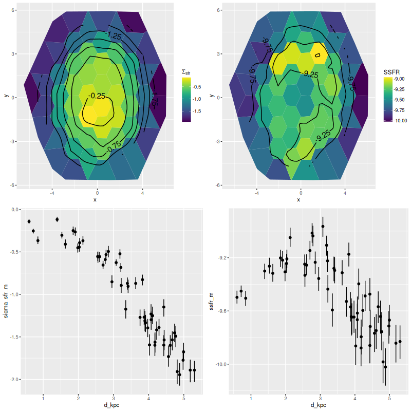
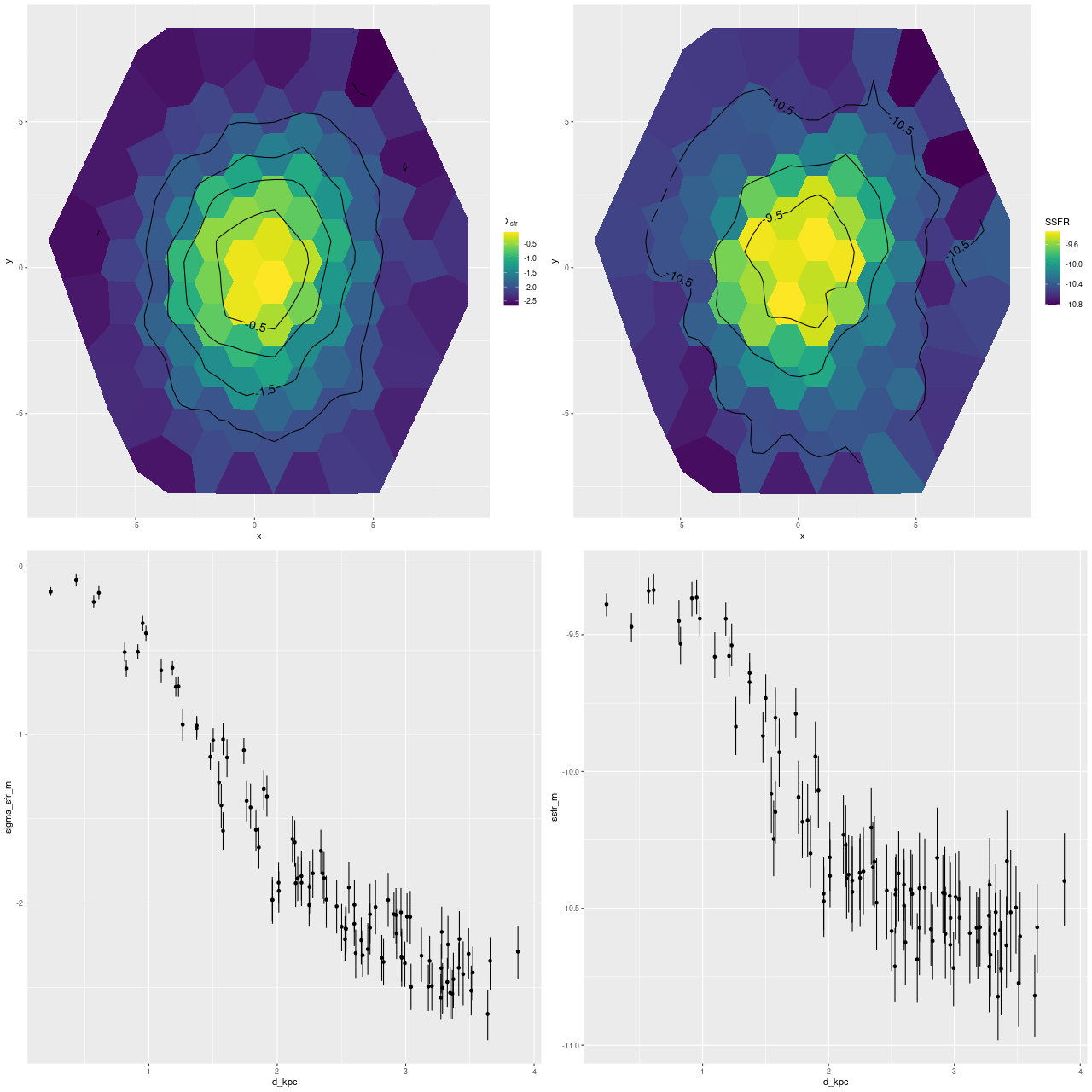
I just want to take a quick look at this one: below are maps of the star formation rate density and SSFR as well as scatterplots of the same against distance from the IFU center. As with MRK 888 ongoing star formation is widespread with a peak near the center, a classic case of a merger fueled starburst. In this galaxy star formation peaks in a ring somewhat outside the nucleus. The ring can be seen clearly in the SDSS cutout and must consist of HII regions.

8095-1902_sfr_ssfr
SDSS J014143.18+134032.8 (mangaid 1-41541; plateifu 8095-1902) Star formation rate density and specific star formation rate – maps and scatterplots against radius in kpc.

Schawinski et al. briefly discuss the possibility that their blue ETG’s could be progenitors of E+A (aka K+A) galaxies. This galaxy and MRK 888 are plausible candidates — if star formation shut off rapidly they would certainly exhibit strong Balmer absorption for a time after emission lines disappeared since they already do. Other members of this sample are already fading towards the red sequence, and if they ever qualified as “post-starburst” it must have been in the past.

I plan to look at star formation histories in more detail after I’ve completed model runs on the MaNGA post-starburst sample.

Adding emission lines to non-parametric kinematic models

This is still experimental and I’m not sure how much farther I’ll pursue it, but I tried a straightforward way to add emission lines to non-parametric line of sight velocity distribution (LOSVD) models. The idea is simple enough: model the line profiles directly using Stan’s simplex data type with each modeled line represented by a vector of mostly zeroes and with the simplex centered on the line’s rest wavelength. Although not essential I’m assuming I will have estimates of redshift offsets for each fiber or spaxel in a MaNGA data file (RSS or cube), so any additional offsets should be small. I’ve chosen to ignore the fact that the discretized line profiles will differ between lines because their central wavelengths will fall at different points within their assigned wavelength bins. Also, different lines could arise from kinematically distinct regions, which is not uncommon in galaxies with broad line AGNs. The obvious solution to this is to allow multiple line profiles. For these initial exercises I’m using a single line profile for all modeled lines (I fit 18 at present). As I’ve done since I started these modeling exercises I am fitting emission lines and stellar contributions simultaneously, with the stellar part represented by a small set of eigenspectra derived from my usual EMILES based library.

Below the “fold” I’ve included the Stan code in it’s current (but certainly not final) form. About half of the code for modeling the stellar LOSVD, is adopted from the original version that I wrote about last year. The emission line model portion takes advantage of an odd feature of Stan, namely the ability to store a matrix in sparse form and perform one specific operation — matrix multiplication with a vector. I still haven’t figured out the particular matrix representation used, so I just create a dummy matrix for the emission lines in the transformed data section and extract the two vectors describing the positions of the non-zero elements of the matrix. In the model section the simplex vector representing the line profiles is repeated as many times as there are lines to fill in the non-zeros.

Another thing to note is that Stan doesn’t know how to work with missing data. In general there will be gaps in spectra that were masked for some reason, while the input templates must be complete over the covered spectrum (plus a few extra at each end for the convolution). This requires a bit of housekeeping that’s mostly done in the R code that sets up the input data.

In the models I ran last year I ignored dust reddening since I didn’t expect it to be significant in the passively evolving Coma cluster galaxies I tested them on. In general reddening isn’t ignorable though and there’s the potential for template mismatch without some allowance for it. For now I inserted the function I use for “modified Calzetti” attenuation but it’s not actually used. In the one test I tried including attenuation in the model significantly increased execution time. I will probably look at using a multiplicative polynomial for the same purpose. A final thing to note is there are no explicit priors for the two simplex vectors that represent the stellar velocity convolution kernel and emission line profile, which means that the priors default to a maximally diffuse dirichlet distribution. This turns out to be an important issue that I will discuss further below.

I’ve run sets of models for a small sample of galaxies so far. so lets look at some results. For these runs I used 500 warmup and 500 post-warmup iterations per chain with 4 parallel chains for a total post-warmup sample size of 2000. The stellar templates are represented by 6 eigenspectra created from singular value decompositions of my standard EMILES based SSP library. I currently fit 18 emission lines — Balmer lines from Hα through Hζ and a selection of the stronger forbidden lines. Model runs typically take 2-3 minutes for sampling on my old 4th generation Intel core I7 based PC. This can undoubtedly be reduced by factors of at least several with multithreading.

In this post I’m going to look in some detail at results for Markarian 888, which was the main topic of my last post. Recall this is one of Schawinski’s “blue early type galaxies” that turns out to have obvious spiral-like structure in its inner region and clear evidence for a relatively recent merger.

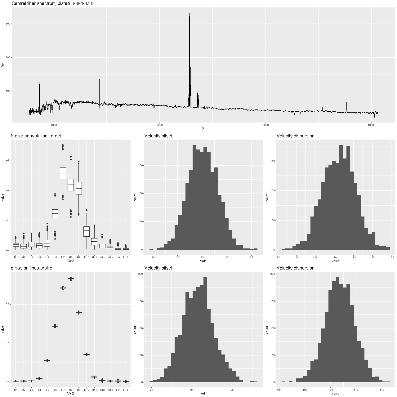
First, the graph below shows the central fiber spectrum, and below that the results of a model run for the stellar velocity convolution kernel. From those I can calculate velocity offsets1these formulas are approximate but close enough for the present purpose.

\( \delta v = 69 \times \sum\limits_{k = -\lfloor K/2 \rfloor}^{\lfloor K/2 \rfloor} k p_i \)

and velocity dispersions

\(
v_{disp} = 69 \times \sqrt{\sum\limits_{k = -\lfloor K/2 \rfloor}^{\lfloor K/2 \rfloor} k^2 p_i – \delta v^2}
\)

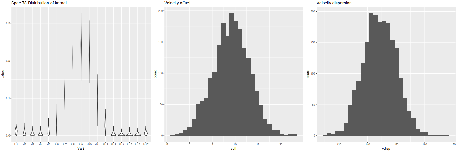
for each draw from the posteriors, and these are shown as histograms in the middle and right graphs. This was a high signal to noise spectrum with prominent emission and absorption lines, a favorable situation for this modeling exercise and in fact the results look very promising with an especially well determined distribution for the emission lines. In summary, the posterior mean stellar velocity offset was 25 km/sec. with a 95% credible interval of (19.8, 31.3), while the corresponding values for emission lines were 24.3 and (22.8, 25.9), so the credible interval for emission lines lies entirely within that for stars.

The corresponding values for velocity dispersions on the other hand differ quite a lot: 141 km/sec. for stars with a 95% credible interval of (133.6, 150.3) versus 109 km/sec and (106, 111) for gas. I’ll say some more about this below, but I think this is already a sign that the second moments (at least) of these velocity distributions need to be treated with caution.

mrk888_centralspec_losv
Markarian 888 – mangaid 9894-3703 Central fiber spectrum, modeled stellar and ionized gas losvd

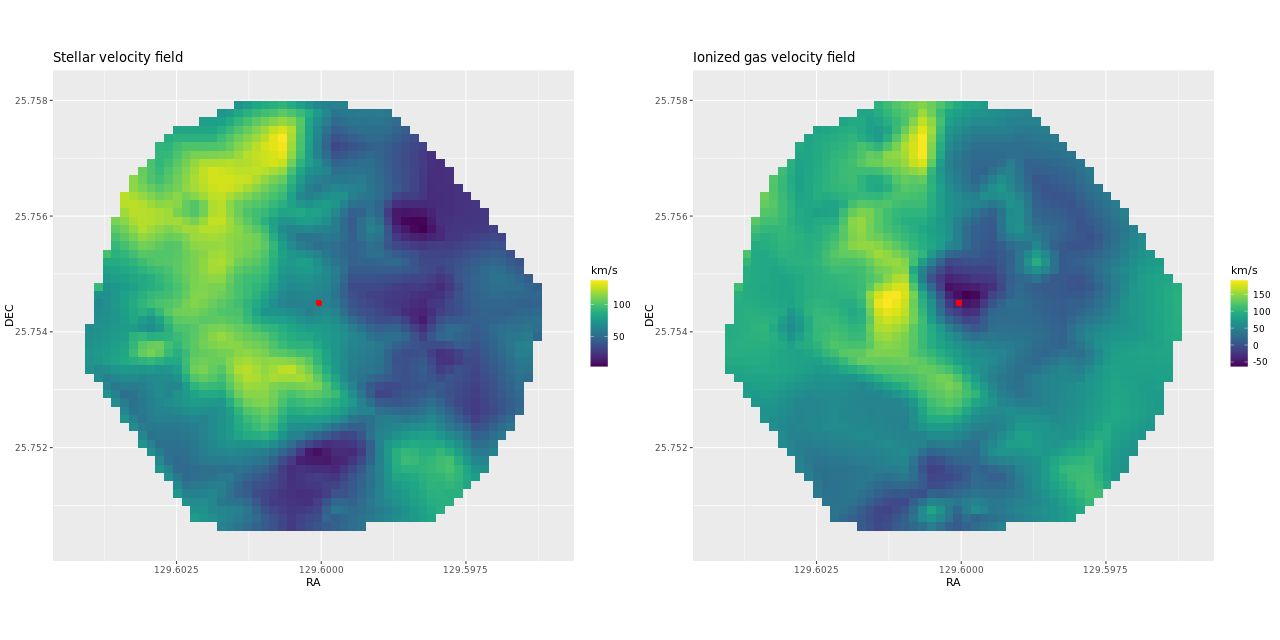
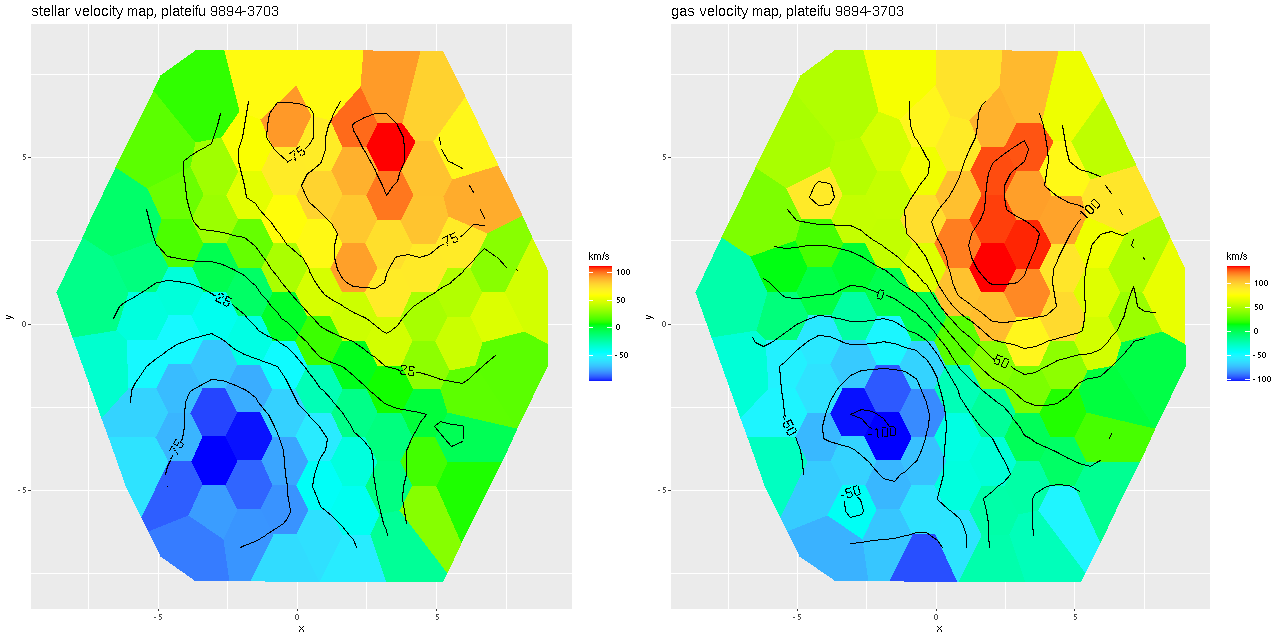
After running the code for every binned spectrum in the IFU I get stellar and gas velocity maps as shown below. These look similar to each other and to the map in the last post based on my hybrid red shift offset fitting routine, although a closer look will show a systematic decoupling of gas and stellar velocities.

mrk888_st_em_losvd
Stellar and ionized gas velocity maps for Mrk 888 (MaNGA plateifu 9894-3703)

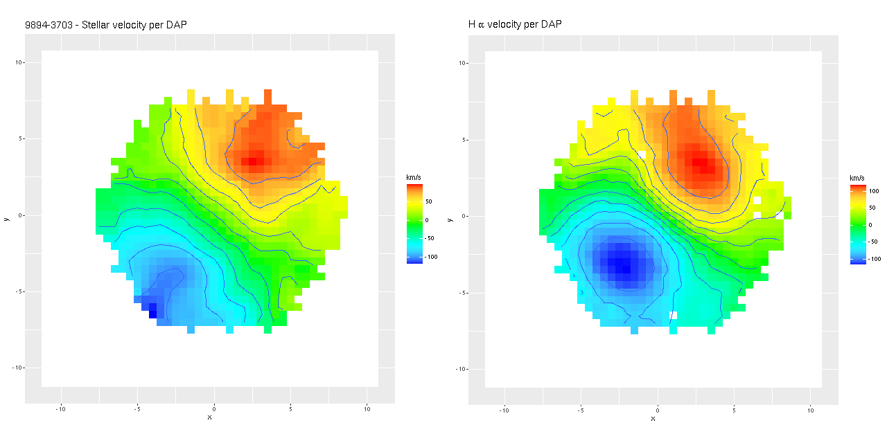
I often take a look at the official MaNGA data analysis pipeline results, usually through the “Marvin” interface. Generally my results look similar for any given quantity, but it’s hard to tell how closely since we’re looking at different things (binned RSS spectra vs. cubes, for one) and I’m really just doing a visual comparison. As more or less a one off exercise I decided to compare velocity fields from the cubes. First, here are stellar and Hα maps from the DAP. These are from the “HYB10-MILESHC-MASTARSSP” sequence, which refers to the binning strategy and template inputs.

mrk888_vel_maps_per_dap
Mrk 888 – stellar and gas velocity fields derived from non-parametric LOSVD models

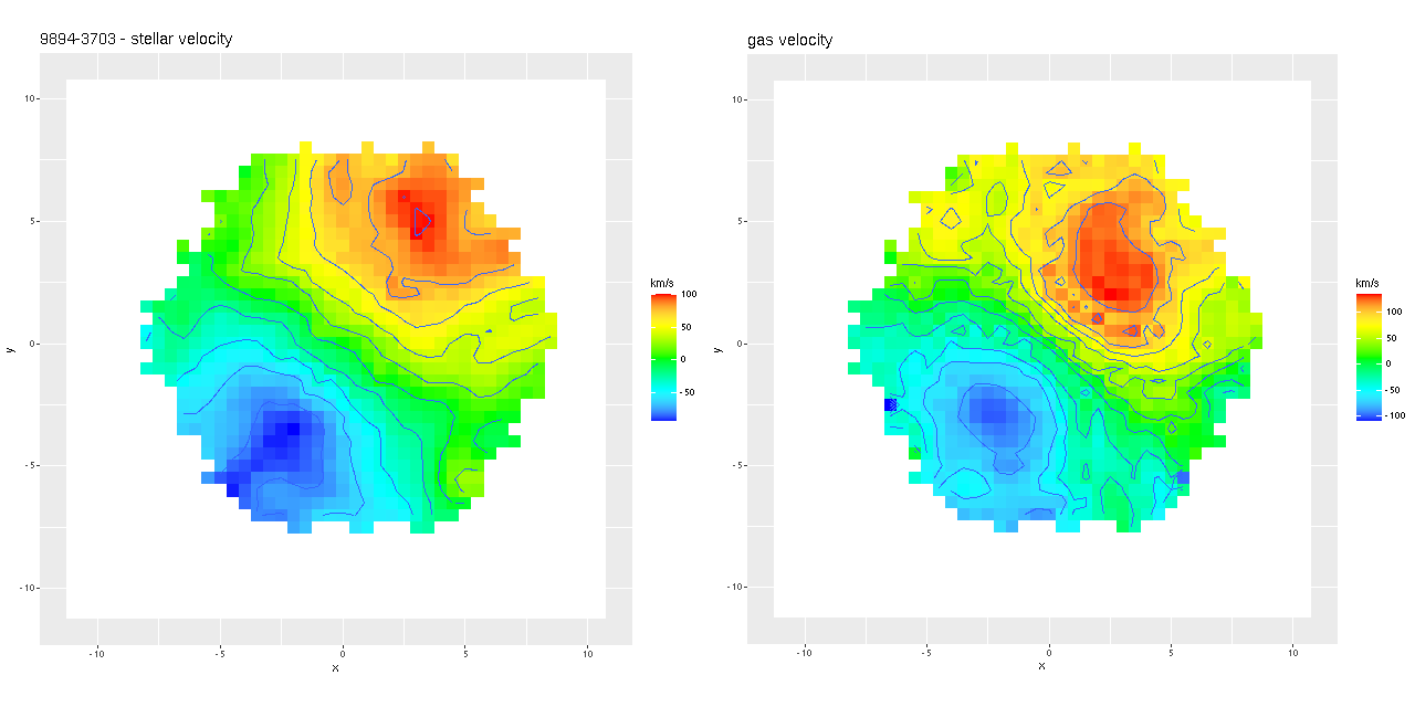
Next are my stellar and ionized gas velocity maps. Evidently these are considerably “noisier” in appearance, but similar overall. The noisiness may be due to different binning strategies: I modeled velocity distributions for every spaxel that met a minimal signal to noise requirement.

mrk888_vel_maps_per_moi
Mrk 888 – stellar and gas velocity fields derived from non-parametric LOSVD models

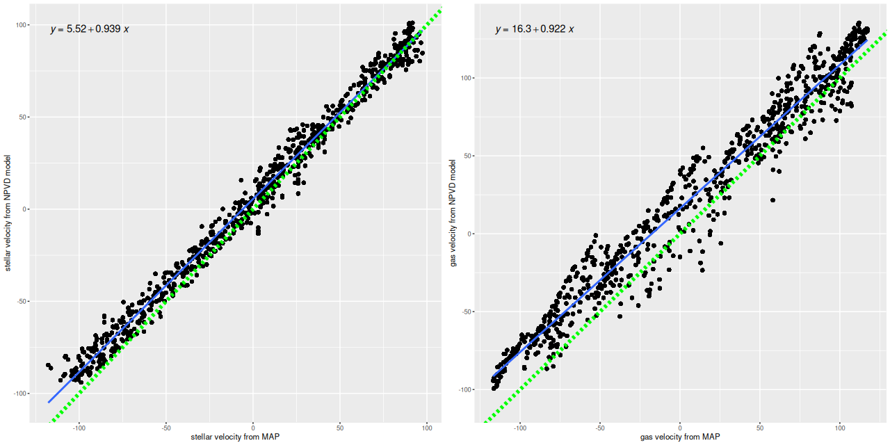
For a more quantitative comparison here are scatterplots of the mean stellar and gas velocity offsets from my runs against the MaNGA DAP. Both of these show slight tilts, that is the slopes are less than one, and small offsets. I’m tempted to suspect systematic errors somewhere, but I haven’t found any yet. And I have no hypothesis about the decidedly non-random behavior of the gas velocity plots. So there are still questions to be answered, but the magnitude of differences is no more than about ±1 wavelength bin (69 km/sec). For my main purposes this is good enough.

mrk888_vel_comp
Mrk 888 – scatter plot of mean stellar and gas velocities – my models vs. DAP

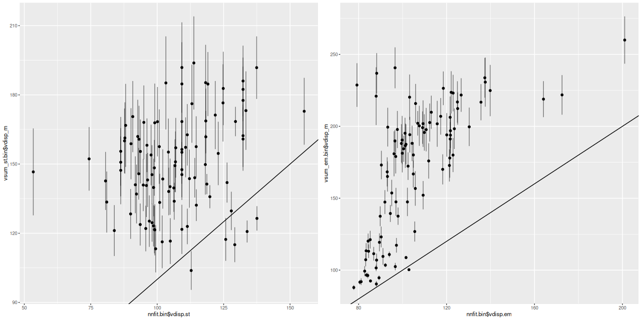
One more pair of graphs for this galaxy. In the initial maximum likelihood fit to a spectrum I estimate stellar and gas velocity dispersions with a single component gaussian. The graphs below plot the velocity dispersions from the Bayesian models calculated by the formula above against the ML fit values. The stellar velocity dispersions behave pretty much the same as I noted before: there’s a weak positive correlation between the non-parametric models and the maximum likelihood estimates with the former generally offset to higher values. The gas velocity dispersion estimates show an even larger discrepancy along with an apparently nonlinear trend.

mrk_888_vdisp
Mrk 888 – velocity dispersions from Bayesian nonparametric losvd models vs. estimates from maximum likelihood fitting

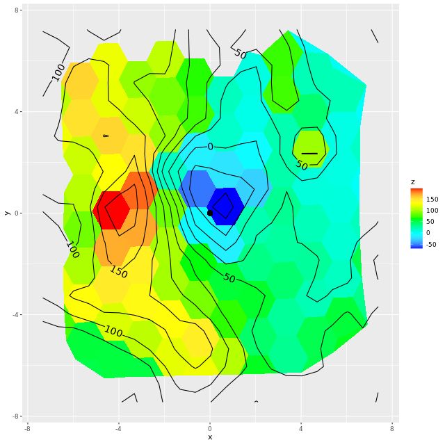
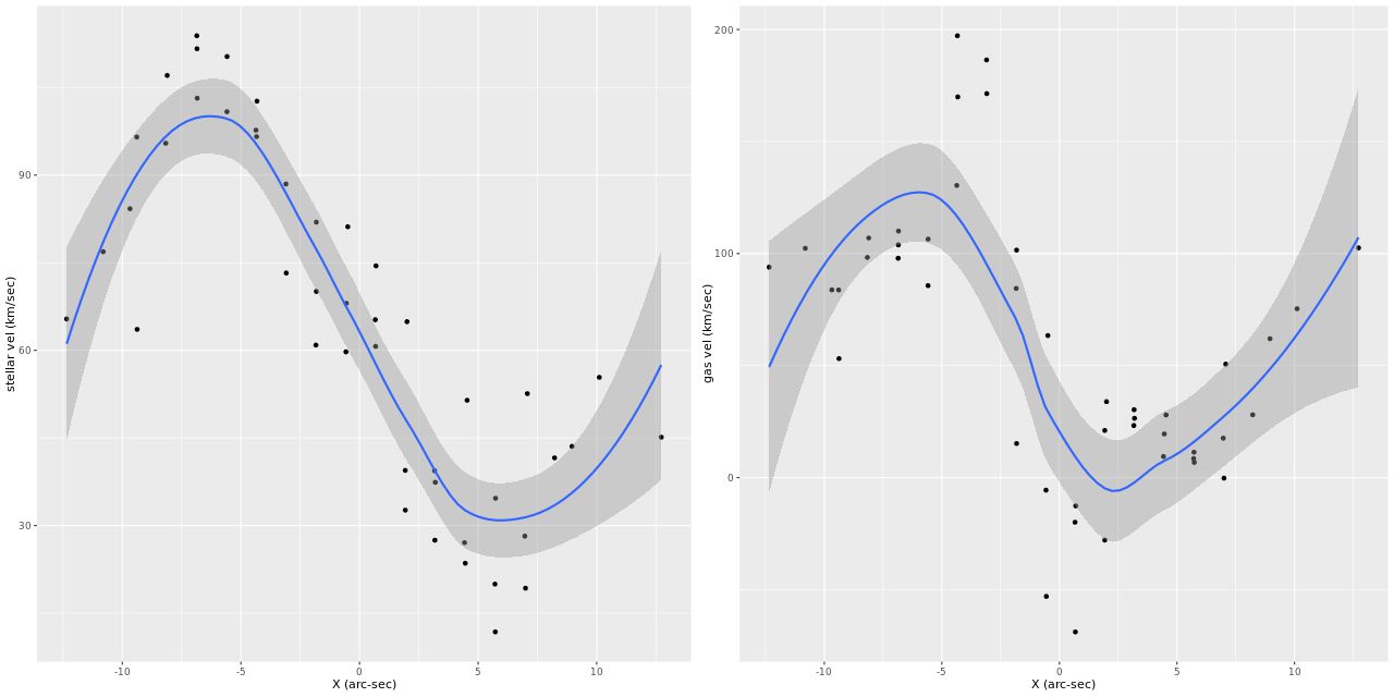
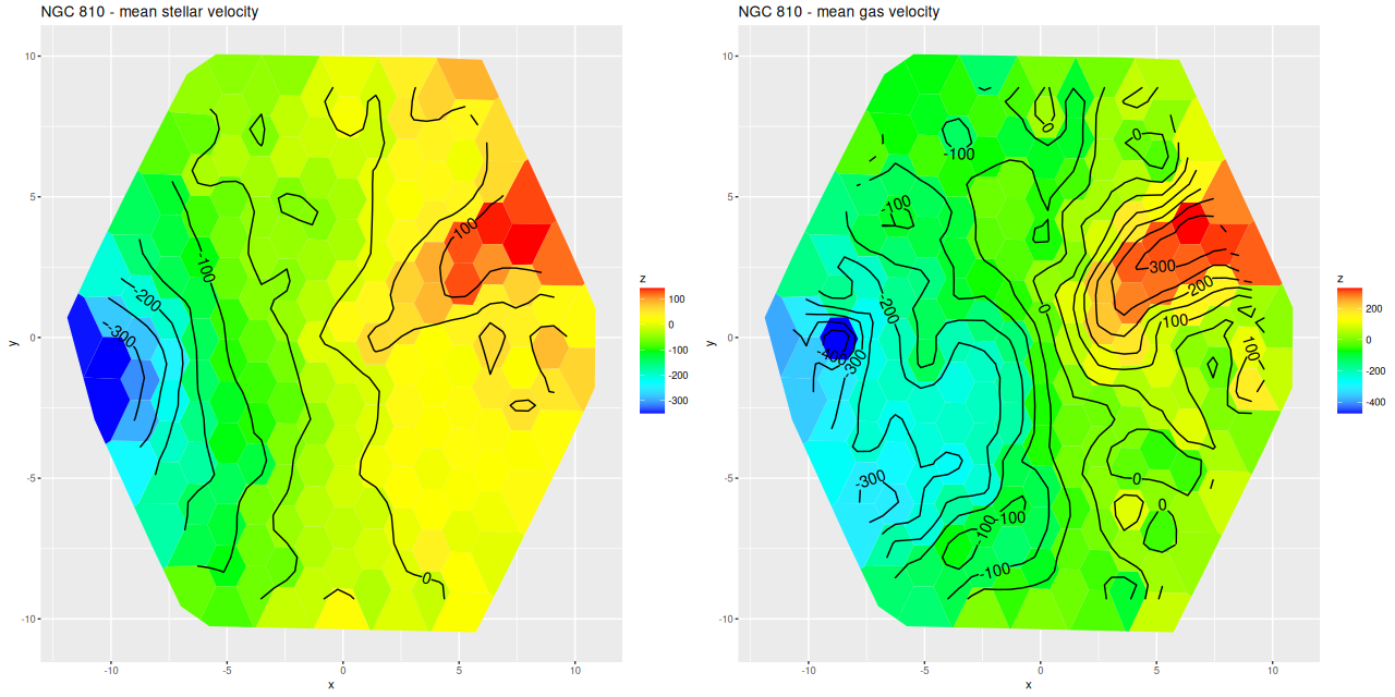
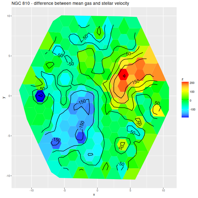
More briefly now, since this got longer than I wanted. I also ran models for the “Zoogems” target NGC 810, which I noted two posts ago has interesting kinematics, in particular a rapidly rotating disk that isn’t evident in the stellar velocity map from the DAP. From the maps below we see that the rapidly rotating component is the ionized gas, which has a mean rotation velocity as much as 150 km/sec larger than the stellar component.

ngc_810_st_em
NGC 810 – mean stellar and gas velocity maps
ngc_810_em-st
NGC 810 – difference between mean gas and stellar velocities

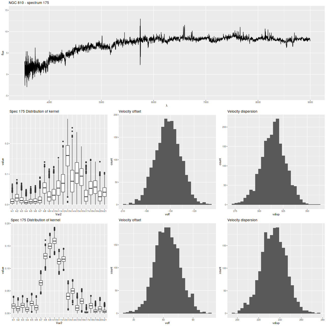
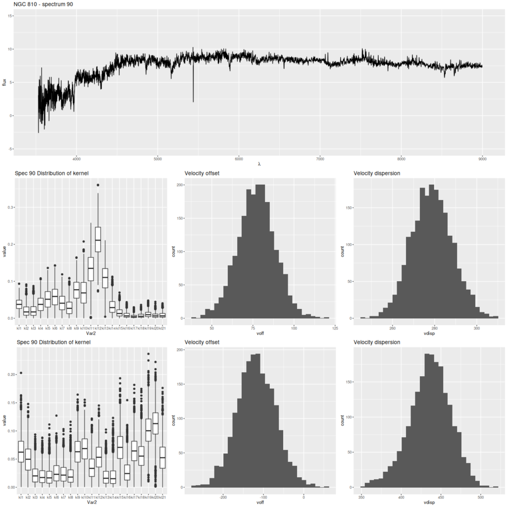
Finally, here are two more graphs of the kinematic models for the spectra with the largest positive and negative differences between stellar and gas velocity (these are the reddest and bluest patches in the map above. These show the spectra in the top row, followed by the posterior distribution of the stellar LOSVD and distributions of the first two moments, then the same for the emission line profiles.

ngc810_175_spec_los
NGC 810 – sample MaNGA spectrum, non-parametric stellar LOSVD and emission line profile
ngc810_90_spec_los
NGC 810 – sample MaNGA spectrum, non-parametric stellar LOSVD and emission line profile

The second set of graphs illustrates a significant problem: when there’s poor data — in this case no detectable emission lines — the models tend to return the prior, which for now is a maximally diffuse dirichlet. This will bias second moment estimates to the high side and can lead to spurious correlations, for example the increase of velocity dispersion with radius that I noted in the last post on this topic.

At the same time this spectrum is in the region of overlap between the main galaxy and its companion, and two peaks in the stellar velocity distribution are clearly seen at about the right velocity offset (~340 km/sec).

A short to do list:

  1. Investigate informative priors.
  2. Allow for dust reddening. I tried using a modified Calzetti attenuation relation in the code (note its presence in the code below, although it’s not used in the model), but it adds too much to execution time. A low order multiplicative polynomial might suffice.
  3. Investigate systematics between my estimates and those in the DAP.

Continue reading “Adding emission lines to non-parametric kinematic models”

What fraction of Schawinski’s “Blue early type galaxies” are ellipticals?

The first iteration of Galaxy Zoo led to several collections of distinct objects, including a sample of 215 “blue early type galaxies” published in Schawinski et al. (2009)1which inexplicably and consistently says there were 204 objects while the catalog published in Vizier contains 215.I found this an interesting group of galaxies, partly because of a possible link to post-starburst (K+A) galaxies that was discussed in the original paper. The authors discuss at some length the likelihood that these are results of mergers in the cosmologically recent past, with at least one of the progenitors being gas rich. Many (at least 25% and possibly more than half) were found to be currently starforming and the rest likely to have only recently ceased forming stars as inferred from their blue colors.

The ongoing Zoogems program has 12 of Schawinski’s blue ETGs on its target list, of which 6 have been observed so far as of mid-January 2022. Somewhat surprisingly there are 24 in the final MaNGA release, over 11% of the sample!

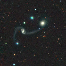
Taking a look at the 6 with HST observations I would say none of these are typical ellipticals. Five show some degree of spiral structure although in 4 it’s embedded in a more diffuse body. One appears to me to be an S0 with both inner and outer rings — this is in agreement with the one published morphological classification I’ve found. All of the others appear more disky than ellipsoidal to me, although this is just my possibly flawed qualitative judgment. At least two are visibly disturbed. One (CGCG 315-014) is connected to a nearby galaxy with a long tidal tail as seen in the Legacy Survey thumbnail below. Markarian 888, which will be the subject of the rest of this post, has shells that extend well past the main body of the galaxy and prominent, centrally concentrated dust lanes.

CGCG 315-014 Legacy Survey Thumbnail

So far it’s the only Zoogems blue etg target with a MaNGA observation (two others on the target list are in MaNGA but of course there’s no guarantee they will ever be observed). As is often the case the IFU could have been larger — this was observed with a 37 fiber bundle giving 111 dithered spectra in the RSS file.

MRK 888 SDSS thumbnail with MaNGA IFU footprint

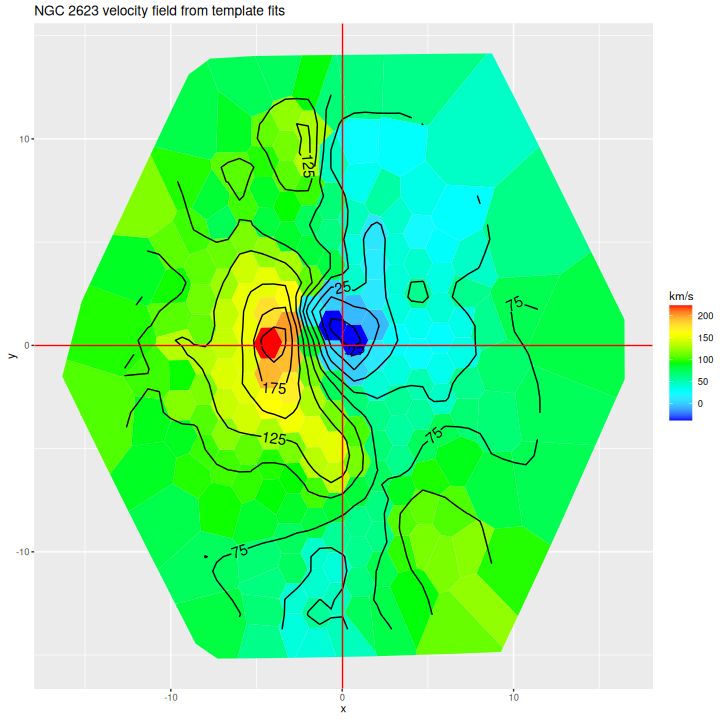
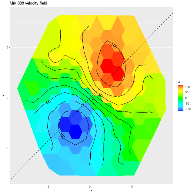
As always the first step in analyzing these data is to estimate redshift offsets for each spectrum, and from there we get a velocity field, which in this case shows a rapid rotator with a fairly symmetrical radial velocity pattern.

Mrk 888 (MaNGA plateifu 9894-3703) velocity field

Visual inspection suggests the line of sight velocity distribution is consistent with a rotating thin disk, so I fed the data to my Gaussian process based rotation modeling code, with results summarized below. In fact the model does an excellent job of accounting for the data, with residuals (not shown) from the model fit (top right) in a range of ±15 km/sec. One unusual feature of the velocity field is the rotation velocity turns over at somewhat less than one effective radius. Whether the rotation curve declines smoothly outside the IFU footprint or is kinematically disconnected from the outer parts of the galaxy is of course unknowable at this time.

Gaussian process rotation model results

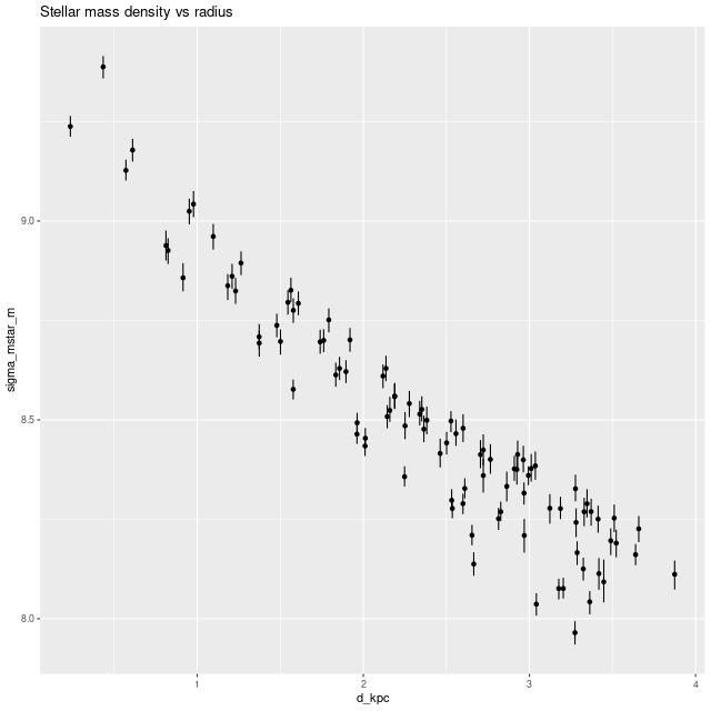
I also ran my usual star formation history modeling code on the data binned to 97 spectra. First, here are some summary results. The stellar mass density declines roughly exponentially, which is consistent with a disky morphology:

Model estimate of stellar mass density vs. radius

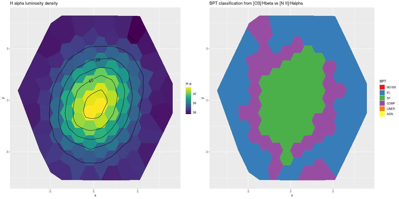
Next are maps of the estimated Hα luminosity density and, on the right, the BPT classification from the [O III]/Hβ vs. [N II]/Hα diagnostic. The contours are elliptical with major axes closely aligned to the rotation axis (the posterior mean for the angle is the dashed line in the velocity field plot above). Again, the emission appears to arise in a disk.

The proper interpretation of the “composite” BPT classification is something I think I’ve written about in the past. It was originally suggested to indicate a mix of AGN and stellar ionization, but here it arises in a thin ring of weak but detectable emission just outside the star forming region. If it’s truly composite it’s likely to arise from a mix of weak star formation and ionization by hot evolved stars. In any case there’s no evidence for an AGN in the optical data.

(L) Hα luminosity density (R) BPT classification from [O III]/Hβ vs {N II]/Hα diagnostic

Next are maps of the modeled (100 Myr average) star formation rate density and specific star formation rate, and in the second row scatter plots of the same estimates against radius in kpc. The trends with radius are somewhat unusual, especially for SSFR which in a normal disk galaxy typically increases with radius even if the highest total star formation rates are centrally concentrated. Highly centrally concentrated star formation in the aftermath of mergers is predicted by some simulations.

(TL) star formation rate density; (TR) specific star formation rate; (bottom row) scatter plots vs. radius

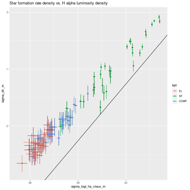
A couple more graphs will round out my discussion of summary model estimates. As I’ve shown several times before there’s a pretty tight linear relationship between modeled SFR density and estimated Hα luminosity density. In this plot Hα is corrected for modeled stellar attenuation, which is expected always to underestimate the attenuation in emission line emitting regions. That, and the fact that Hα emission and the model star formation rate estimates probe order of magnitude different time scales probably account for the systematic offset from the standard calibration given by the straight line.

Model star formation rate density vs. Hα luminosity density corrected for stellar attenuation. Straight line is calibration from Calzetti (2012).

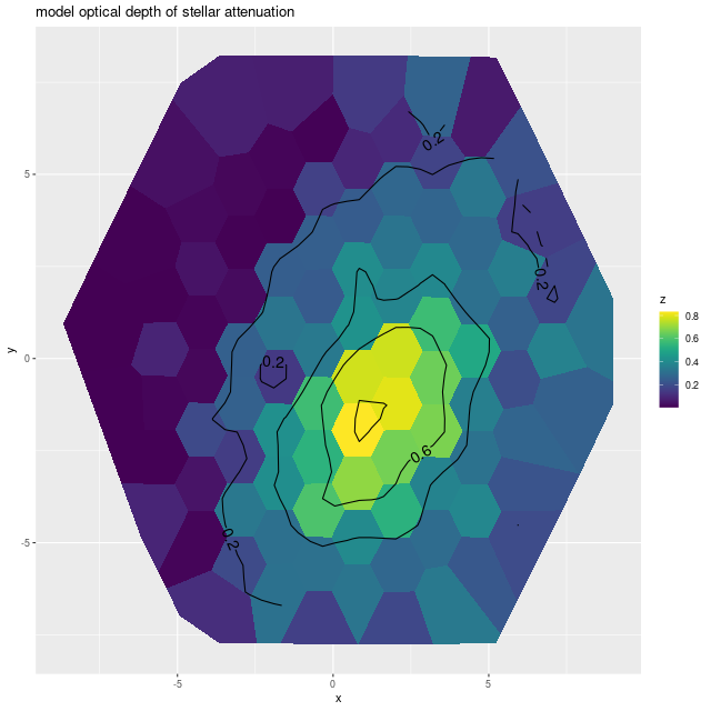
And, once again I show a map of the modeled optical depth of stellar attenuation. The region of highest optical depth nicely tracks the visible dust (the HST image at the top is rotated about 90º from the SDSS image). Outside the dusty region there appears to be a shallow gradient, which might indicate that the nearer side is to the northeast.

Map of modeled optical depth of stellar attenuation

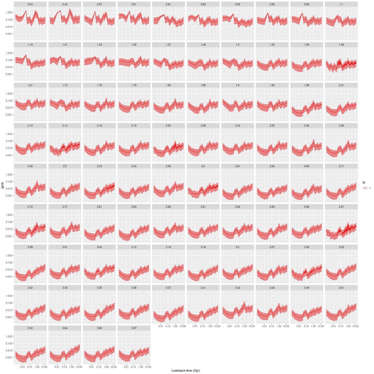
Finally here are plots of the model star formation history for all spectra ordered by distance from the IFU center. In the inner 1.5 kpc or so there’s some recent burstiness with possibly a very recent acceleration of star formation. For reasons I’ve discussed recently I don’t take either the timing or magnitude of bursts of star formation too seriously, but the behavior of the models is consistent with a recent revival of star formation due presumably to a merger, for which there are multiple lines of evidence.

model star fomation histories for all spectra

With 24 of these galaxies and another 31 from the compilation of Melnick and dePropris and the post-starburst ancillary program in the final release of MaNGA these samples satisfy my criteria of being manageably sized for my computing resources while large enough to say something about the groups. So, when time permits I plan to take a look. I already have the data in hand.

NGC 810 – interesting kinematics in a Zoogems and MaNGA target

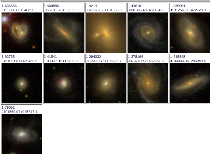
The final release of SDSS MaNGA went public back in early December as promised, and I’ve spent the last month or so of my hobby time looking for manageable sized samples of interesting galaxies. One sample I looked at out of curiosity was the Zoogems target list, which is an HST gap filler imaging program with about 300 galaxies selected (mostly) by Galaxy Zoo volunteers. It turns out there are 11 targets with MaNGA data, of which 5 have been observed by HST so far.

thumbnails
SDSS thumbnail images of Zoogems targets with MaNGA data

As can be seen from the thumbnails above this is a pretty diverse lot, with several in progress mergers and merger remnants, some normal looking spirals at least two of which were from Masters’ red spirals sample, and 3 of Schawinski’s blue early type galaxies. Only one of those 3 has HST imaging so far (number 8 in the thumbnails above), although there are a surprising 24 blue ellipticals in the final MaNGA release out of 215 in Schawinski’s original sample.

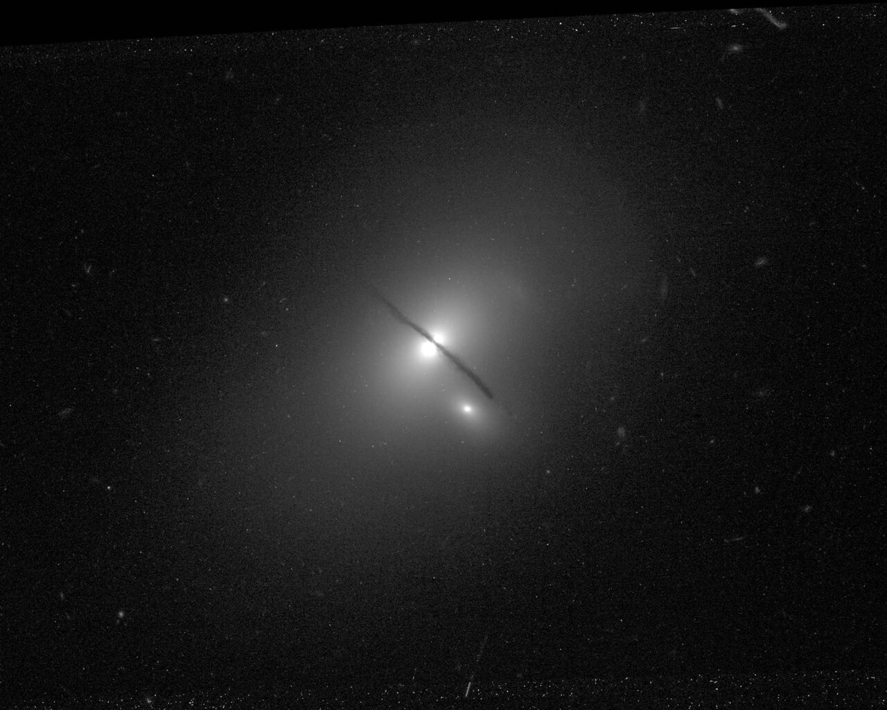
Of the 5 Zoogems galaxies that have been observed so far the one that caught my eye as deserving an early look was number 3 in the top row, NGC 810, an apparent elliptical with an unusual dust lane that’s almost perfectly aligned with the minor axis. There are also hints of shells indicating a likely merger sometime in the past.

NGC 810 HST ACS, proposal id 15445, PI Keel

The MaNGA data, which is new in DR17, only covers the central part of the galaxy with the companion just photobombing the edge. A larger IFU would have been nice for this observation, but the data quality is better than average in terms of nominal signal to noise. I was able to use all 183 fiber/position combinations in the RSS file without binning.

NGC 810 – plateifu 9514-6101 – MaNGA IFU footprint

The first step in the analysis process after loading the data is to estimate redshift offsets from the system redshift for each spectrum, and from that it’s straightforward to calculate a velocity field, which in this galaxy looks like1this is actually from the data cube:

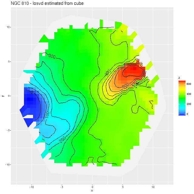
NGC 810 (plateifu 9514-6101) – losvd estimated from cube

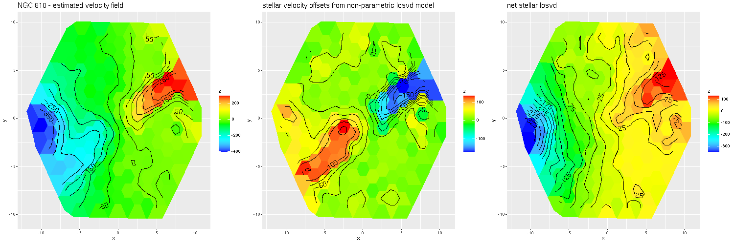
It turns out the redshift assigned to this system was that of the companion galaxy, which was the only SDSS spectroscopic target in the immediate vicinity and is evidently blueshifted by ~350 km/sec from the target. What’s more interesting though2interesting enough that I made a couple posts on the Galaxy Zoo talk forum, which I rarely do anymore. is the apparent rapidly rotating disk that’s aligned with and somewhat thicker than the dust lane. There may also be overall prolate rotation outside the disk although the presence of the companion makes it hard to tell based solely on visual inspection. In hopes of separating out multiple velocity components I returned to the non-parametric line of sight velocity distribution models that I wrote some posts about last year. Unlike the ones I practiced on previously this galaxy has non-negligible amounts of emission, at least in the central region, so I just temporarily masked the regions around the emission lines that I fit. That results in a pure stellar velocity distribution. The results were a bit surprising:

NGC 810 (plateifu 9514-6101) (L) velocity field estimated from RSS file (M) stellar velocity offsets (R) net stellar velocity

In the left pane above is the velocity field from the RSS data, with the system redshift adjusted to the IFU center. For the LOSVD models I set the adopted redshift of each spectrum to the system redshift plus the offset calculated previously. Now I had hoped to be able to cleanly separate the contribution of the companion from that of the main galaxy, which so far I haven’t been able to do. But what I did find that was unexpected is that the average stellar velocities in the disk partially offset the original measurements (middle pane), so the net stellar velocity field shows a much more slowly rotating stellar disk.

As I’ve written before I use a set of 15 eigenspectra from a principal components analysis of some tens of thousands of SDSS spectra that I performed some years ago for redshift offset estimation. Those galaxies were of all types and include systems both with and without significant emission. The redshift estimation routine just does straightforward template matching and returns a single value for the best fitting offset. Since the templates encode information about both emission and absorption lines that estimate could be most applicable to the ionized gas, stars, or some combination. In this case it’s possible emission lines were driving the original fits, implying the gas and stars in the disk are kinematically decoupled. I have not verified that though.

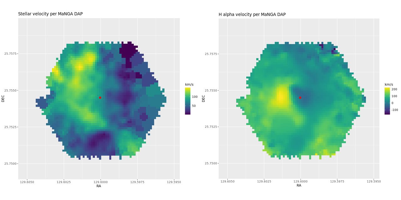
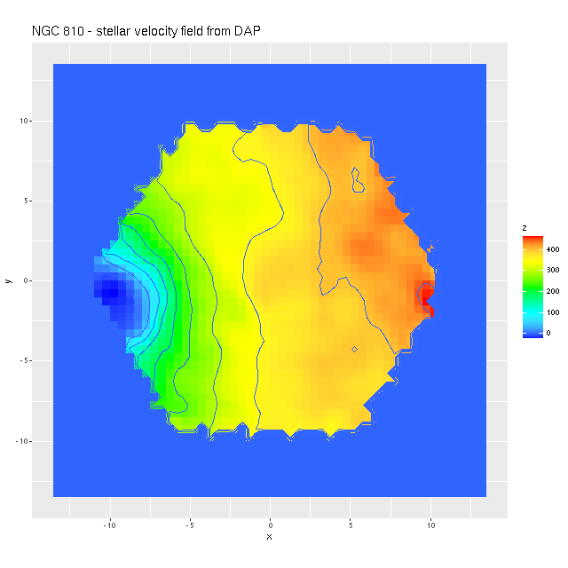
Another issue I noticed is that the stellar velocity field from the official MaNGA Data Analysis Pipeline looks rather different from mine, with barely a hint of a kinematically distinct disk. This wasn’t really evident in the Marvin webpage, which makes some really unfortunate choices for color palettes. So here is the same data rendered with a more nearly perceptually uniform rainbow palette3I know data visualization experts frown on rainbows, but I think they’re OK for things like velocities or redshifts:

NGC 810 (plateifu 9514-6101) Stellar velocity field per MaNGA DAP

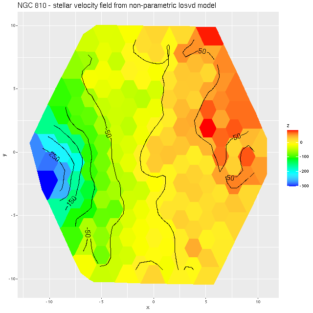
I decided to re-run my LOSVD modeling code on the RSS data, this time setting the redshift offset to 0 for each fiber, so this is now measuring velocities relative to the overall system velocity. I also used a larger convolution kernel (25 vs. 21 in the first set of runs). The map of the average velocity offsets is:

NGC 810 (plateifu 9514-6101) Stellar losvd from nonparametric model

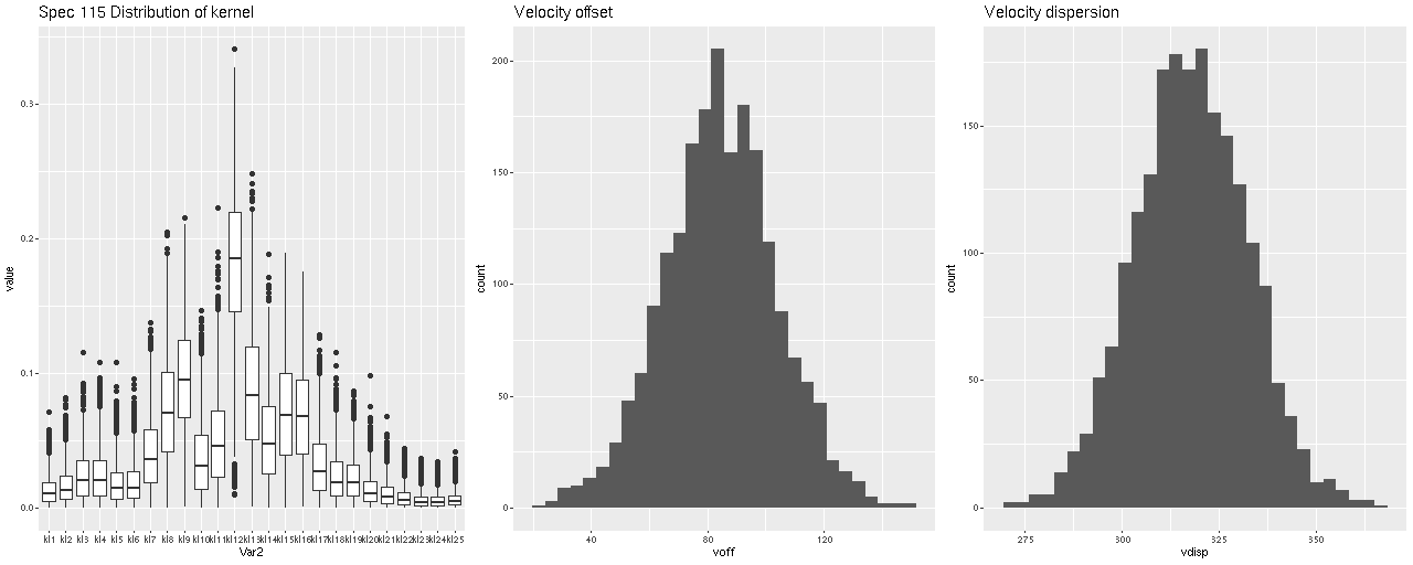
Although not a perfect match this is somewhat closer to the DAP map. I suspect what’s happening here is that there really are at least two, and more likely 3 distinct kinematic components. I haven’t read the DAP release paper in a while and don’t know exactly how they estimate stellar velocities, but in any case their model just returns a single value for visualization purposes. To see the (possible) complexity of the actual data here are the results for a single fiber with the largest positive velocity offset in the map above. Again, I don’t know how much of the structure in the posterior distribution of the convolution kernel is real, but it’s evident there’s more complexity than is captured in the first two moments shown in the middle and right panes.

NGC 810 – sample nonparametric losvd

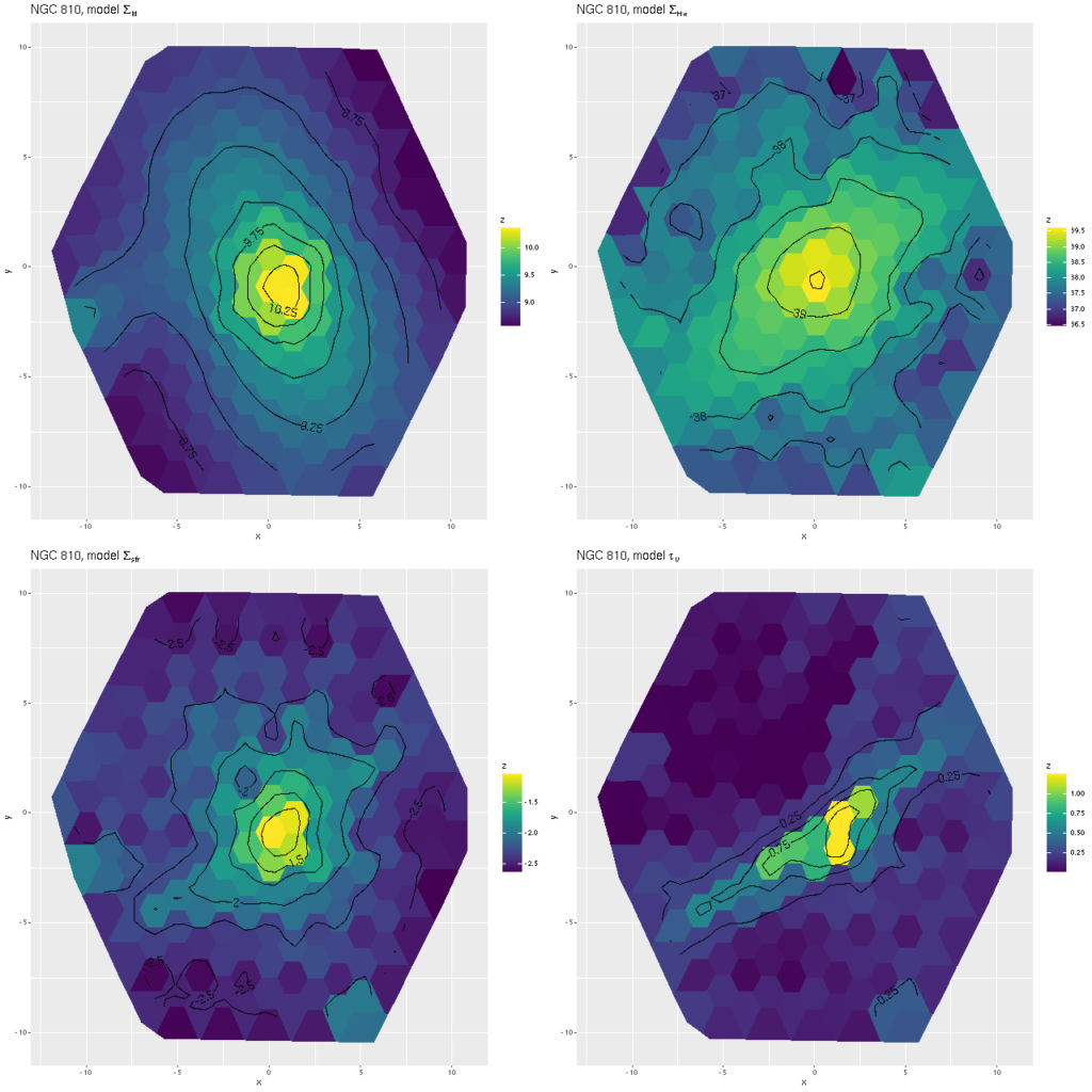
Besides the kinematic modeling I did run star formation history models on the full RSS data set using the same tools as in recent posts. I’m not going to discuss them in detail, but some summary maps are worth showing. In the graphic below these are, from top left, stellar mass density, Hα luminosity density uncorrected for attenuation, SFR density (as usual 100Myr average), and stellar dust attenuation.

There’s no sign of a disk in the stellar mass map, which faithfully follows the distribution of light. A disk is visible in Hα and the small amount of recent starformation is also confined to a disk and nuclear region. In the fourth pane I show the modeled stellar dust attenuation, mostly just to demonstrate that this component of the model does capture something of reality.

ngc810_model_summaries
NGC 810 – a sampling of quantities derived from star formation history models

Getting back briefly to the first paragraph, there are 8 post-starburst galaxies from the catalog of Melnick and de Propris and 24 from an ancillary program to observe post-starburst galaxies from various sources that was added for DR17. There’s just one galaxy from the former catalog in the latter set, so that makes 31 total, an easily manageable number. There are also 24 of Schawinski’s blue ellipticals. Of course there are many disk galaxies, far too many for me to look at.

Continue reading “NGC 810 – interesting kinematics in a Zoogems and MaNGA target”

KUG 0859+406 – unravelling the differences between 2018 and 2021 model runs

I did have my old data and model runs of course, in fact they were spread over several directories on two machines. I’m going to refer to it by this catalog designation, KUG standing for the “Kiso survey of Ultraviolet-excess Galaxies.” It’s also a low power radio source with catalog entries in both FIRST and NVSS, and of course it’s in MaNGA with plateifu ID 8440-6104 (mangaid 01-216976).

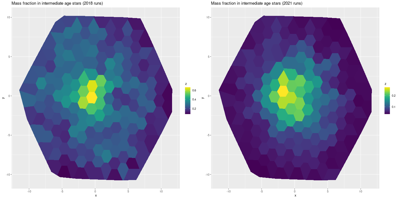
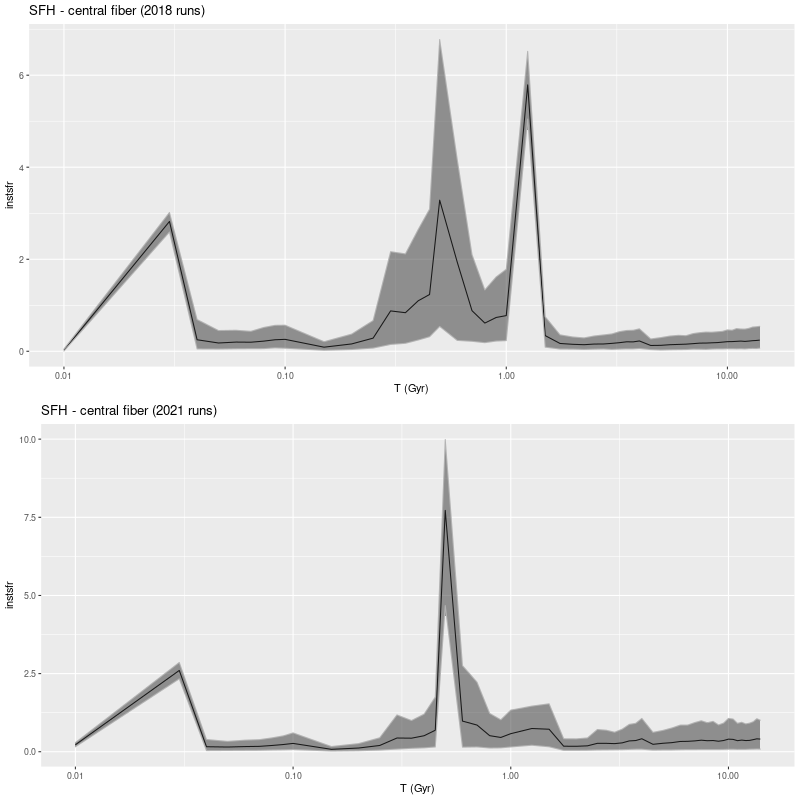
In my 2018 model runs, which were interesting enough to write 3 posts about, I found this galaxy had undergone an extraordinarily large burst of star formation that began ~1 Gyr ago with locally as much as 60% of the present day stellar mass born in the burst and something like 40% of the mass over the footprint of the IFU. In this years model runs the peak burst fraction was a considerably more modest ~25% and globally barely amounted to a slight enhancement of star formation. The starburst was also much more localized than in the earlier runs:

burst_strengths_compared
Fractional stellar mass in stars between 0.1 and 1.75 Gyr old in 2018 and 2021 model runs

So what happened? First, here is a comparison of modeled star formation histories for the innermost fiber, which got the largest injection of mass in the starburst.

central_sfh_compared
Model star formation histories for central fiber of MaNGA plateifu 8440-6104, 2018 and 2021 model runs

The obvious remark is the double peaked starburst noted back in 2018 (and discussed at some length) has been replaced with a single narrow peak with a slow ramp up and fast decay. The peak SFR is a little larger than before but the total mass in the burst is lower.

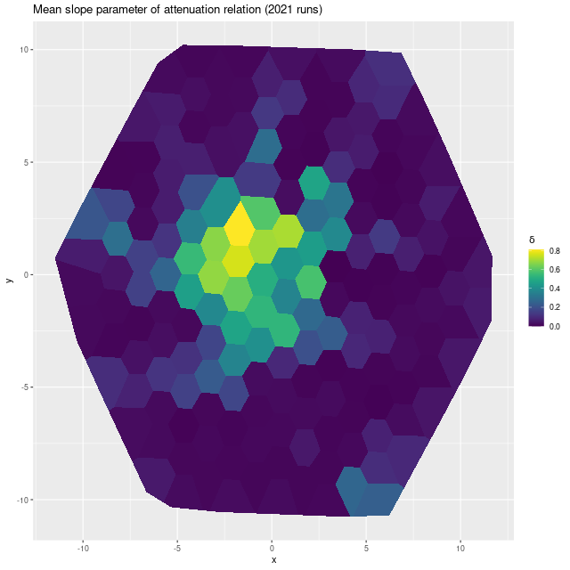
I’ve made several changes in model formulation since 2018, of which the most important in the current context is adopting the more flexible “modified Calzetti” attenuation relation that adds an additional slope parameter to the prescription. In the current year model runs a steeper than Calzetti relation is favored throughout the IFU footprint, particularly in the central region where the starburst was strongest:

map_delta
Map of modified Cal;zetti slope parameter δ — MaNGA plateifu 8440-6104

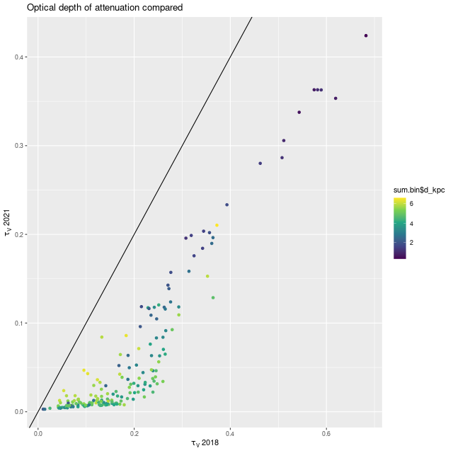
A smaller optical depth of attenuation is also favored throughout:

tauv_compared
Modeled optical depth of attenuation – 2021 runs vs. 2018 MaNGA plateifu 8440-6104

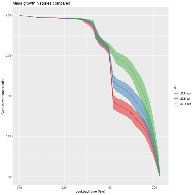
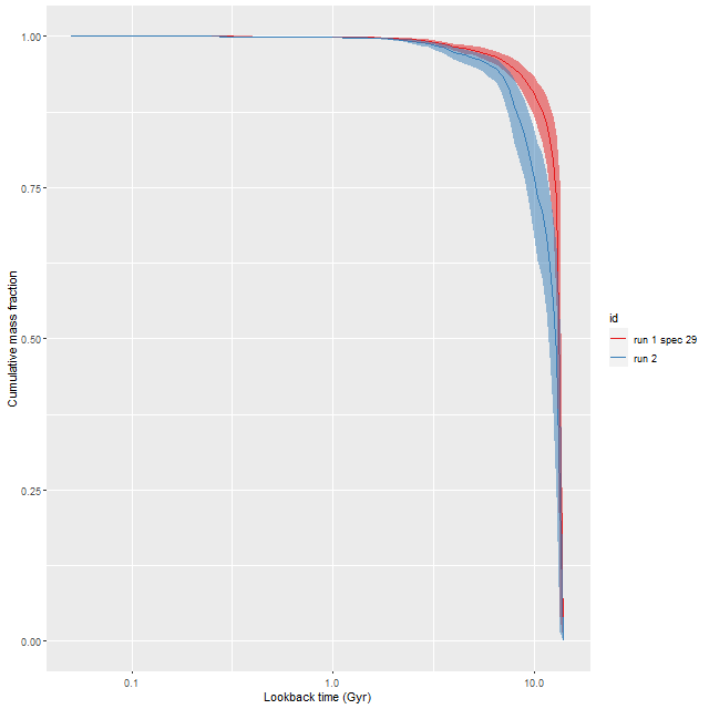
This has a couple predictable consequences. Steeper attenuation will favor an intrinsically bluer, hence younger population while a lower optical depth requires less light, and hence mass in the stellar population. I can test this directly by returning to a model with Calzetti attenuation, and here is the result for the central fiber (this model run is labeled 2021 (c) in the legend below):

mgh_compared
Mass growth histories – 2021 run 2021 run with Calzetti attenuation 2018 run Central fiber of MaNGA plateifu 8440-6104

So, an eyeball analysis suggests about 3/4 of the difference between the 2018 and 2021 runs is due to the modification to the attenuation relation. The other changes I’ve made to the models are to change the stellar contribution parameters from a non-negative vector to a simplex, and at the same time changing the way I rescale the data. In early runs the SSP model fluxes were scaled to make the maximum stellar contribution ≈ 1, while the current models scale both the galaxy and SSP fluxes to ≈ 1 in the neighborhood of V, making the individual stellar contributions approximately the fraction of light contributed. An additional scale factor parameter in the model is used to adjust the overall fit. Assuming I did this right this should have no effect on a deterministic maximum likelihood solution, but with MCMC who knows?

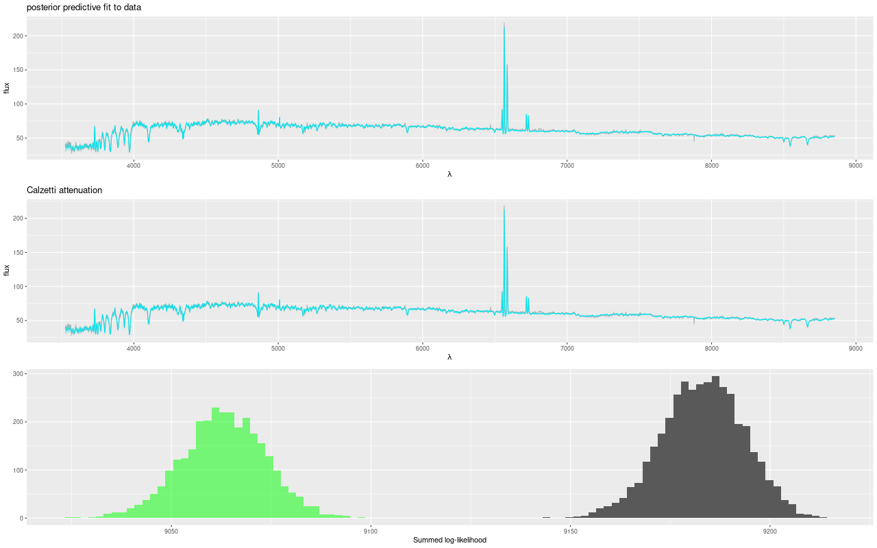
Although the fit to the data looks about the same between the model with and without the attenuation modification the summed log-likelihood is consistently about 1% higher for the modified Calzetti model with no overlap at all in the distribution of likelihood. This suggests the case for a steeper than Calzetti attenuation is a fairly robust result.

ppfits
“Posterior predictive” fits to galaxy flux data – modified Calzetti attenuation vs. Calzetti – central fiber of MaNGA plateifu 8440-6104

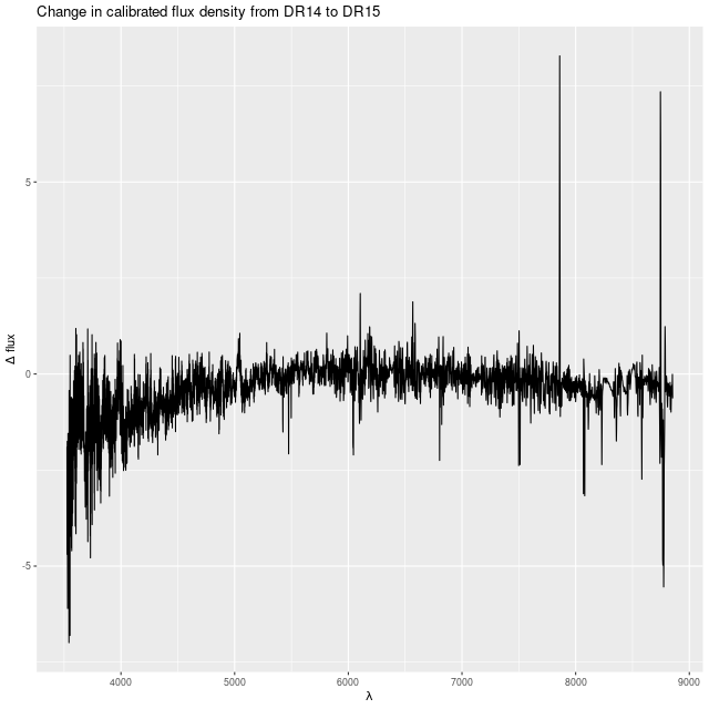
The galaxy flux data also changed a little bit. The early runs were on the DR14 release (version 2_1_2 of the MaNGA DRP) while the recent ones used the DR15 release (ver 2_4_3). Most of the calibration differences resemble random noise, but there is some curvature that systematically affects both the red and blue ends of the spectrum and could cause some change in the temperature distribution of the models:

measured_flux_compared
Difference in measured flux from DR14 to DR15 – central fiber of MaNGA plateifu 8440-6104

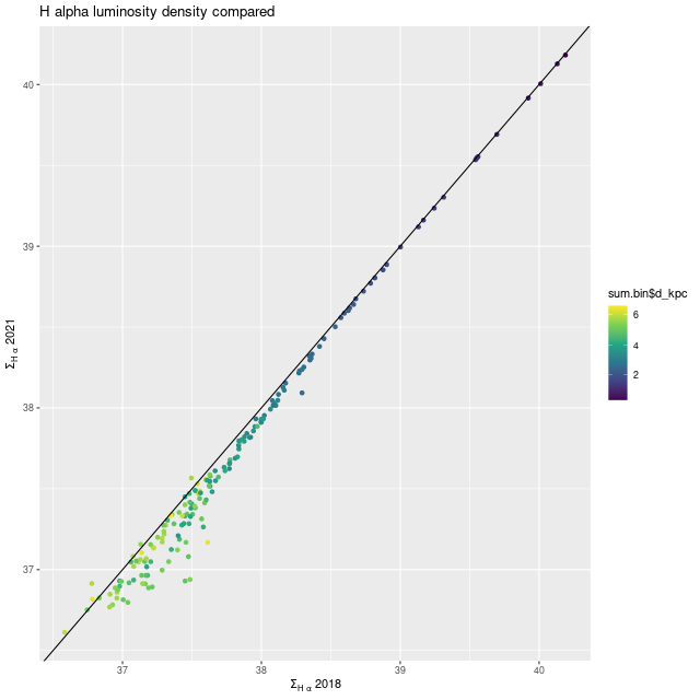
While the detailed star formation histories changed, quantities that aren’t too model dependent didn’t very much. One example is shown below. Also, the kinematic maps agree with the earlier ones in detail.

halpha_luminosity_compared
Hα luminosity density – 2021 runs vs. 2018 MaNGA plateifu 8440-6104
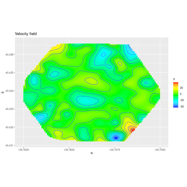
velocity_field_8440_6104
Velocity field of MaNGA plateifu 8440-6104 from 2021 model runs. Map interpolated from RSS file spectra.

One input that hasn’t changed are the emiles SSP model spectra, although there have been some procedural changes in how I handle the modeling. Early on I often used a much smaller subset of SSP models with just 27 time bins and 3 metallicities for preliminary modeling, including my first models on the same binning of these data. I also routinely ran 250 warmup iterations with just 250 more per chain. My current standard practice is always to use the largest emiles subset with 216 SSP models in 54 time bins and 4 metallicities, and I generally run 750 post-warmup iterations per chain but still with only 250 warmup iterations. This is generally enough and if adaptation fails it is usually fairly obvious. The small sample size of the earlier runs mostly effects the precision of inferences rather than means.

To conclude for now, my speculation about whether it might be possible to say something about the timing of critical events in a merger from the model star formation history was too optimistic. On a positive note though both sets of model runs retrodict that coalescence occurred at a lookback time around 500Myr ago, which is consistent with the fact that tidal tails and other merger signatures are clearly visible even in SDSS imaging. Both sets of model runs also have that odd uptick in star formation at 30Myr in the central fiber. And while the difference in burst mass contributions is a little disconcerting the current runs are more consistent with the likely gas content of ordinary spiral galaxies.

This example illustrates another well known “degeneracy” among attenuation (and adopted attenuation relation), mass, and stellar age. Whether I’ve broken the degeneracy by adopting the more flexible attenuation prescription described some time ago remains to be validated.

Do the details of the line of sight velocity distribution matter for star formation history modeling? Probably not much.

I decided to try a set of models for one galaxy – NGC 4889 (with MaNGA plateifu 8479-12701), which had the highest overall velocity dispersion of the Coma sample I’ve been discussing in the last several posts. It also has some evidence for multiple kinematic components which isn’t too much of a surprise since it’s one of the central cD galaxies in Coma. The SSP model spectra fed to the SFH models were preconvolved with the element wise means of the LOSVD convolution kernels from the velocity distribution modeling exercise. Again, this is an expedient to avoid what could otherwise be prohibitively computationally expensive. The models I ran were the same as described back in this post — these ignore emission but do model dust attenuation with the usual modified Calzetti attenuation relation.

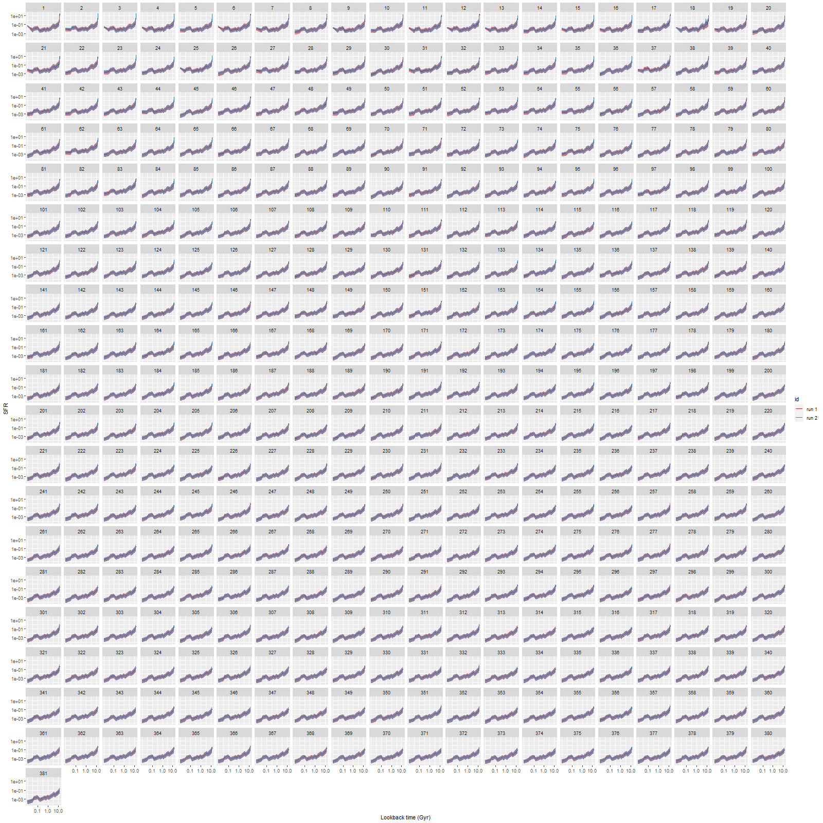
To get quickly to the results, here are model star formation histories compared to the previous runs that used the full model in its current form. Usually I like these plots of results from all spectra in an IFU, but in this one all 381 spectra met my S/N criterion, so the plot is pretty crowded. You really need to see it live on a 4K monitor to see the details.

NGC 4889 (MaNGA plateifu 8479-12701) Model star formation histories for all spectra, runs with non-parametric LOSVD vs. single gaussian stellar velocity dispersions

Well it’s pretty hard to see but differences in model SFH’s are mostly in the youngest age bins, which are very poorly constrained anyway in these presumably passively evolving galaxies. Here’s a closer look at a single model run that had the largest difference in estimated stellar mass density (more on this right below) of about 0.19 dex:

mgh_comparison_8479-12701
NGC 4889 (MaNGA plateifu 8479-12701) Model mass growth histories for a single spectrum – runs with non-parametric LOSVD vs. single Gaussian stellar velocity dispersion

So, the difference in star formation histories was slower mass build up between about 12-5 Gyr look back times in the second run, which was responsible for the lower current day stellar mass density. How this resulted from the choice of LOSVD is not at all obvious.

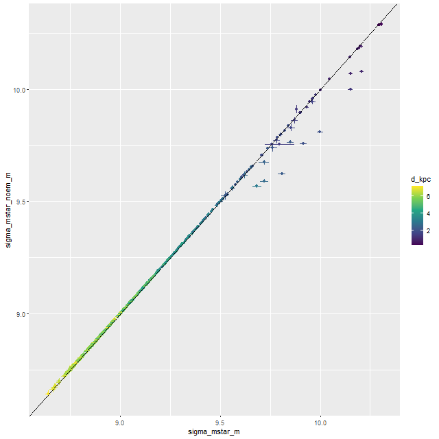
Let’s look at a few summary results. First, the model stellar mass surface densities:

sigma_mstar_comparison_8479-12701
NGC 4889 (MaNGA plateifu 8479-12701) Model ΣM* – runs with non-parametric LOSVD vs. single Gaussian stellar velocity dispersion

These fall on an almost exactly one to one relation with a few hands full of outliers. Oddly these are mostly in the higher signal to noise area of the IFU (i.e. near the center).

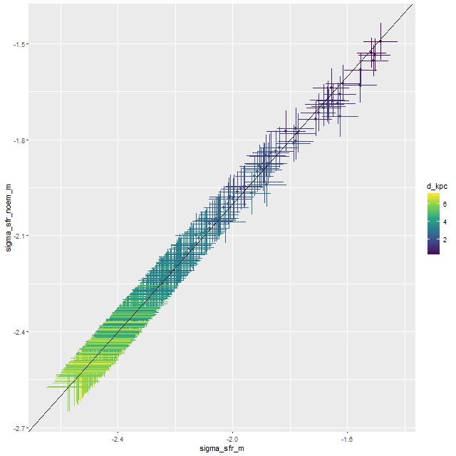
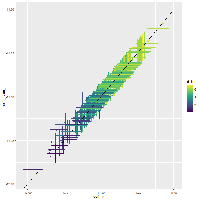
Results for star formation rate density and specific star formation rate are even more consistent between runs, with essentially no differences larger than the nominal 1 σ error bars.

sigma_sfr_comparison_8479-12701
NGC 4889 (MaNGA plateifu 8479-12701) Model Σsfr – runs with non-parametric LOSVD vs. single Gaussian stellar velocity dispersion
ssfr_comparison_8479-12701
NGC 4889 (MaNGA plateifu 8479-12701) Model SSFR – runs with non-parametric LOSVD vs. single Gaussian stellar velocity dispersion

One problem I encountered was that I had to re-run some models either for technical reasons or because of obvious convergence failures. I suspect there could have been some convergence issues in both sets of runs and am slightly worried that could be the source of the few differences in summary measures seen. Oddly, there were almost no suspicious convergence diagnostics in either set of runs (once the latter were run to satisfactory conclusion), and Stan is quite aggressive about reporting possible convergence issues.

Anyway, modeling kinematics remains an interesting topic to me, but it seems somewhat decoupled from modeling star formation histories. Right now I’m waiting for the final SDSS data release to decide what projects I want to tackle.

I’m going to end with a couple of asides. First, I recognize that all of these error bars are overoptimistic, maybe by a lot. The main reason, I think, is that I treat the flux values as independent which they clearly are not1 this is pretty standard practice however, which effectively results in overestimating the sample size. One possible partial solution is to allow the flux uncertainties to vary from their nominal values by, for example, a factor > 1. This would involve adding as few as one parameter to the models, which is something I’ve actually tried in the past. I may relook at that.

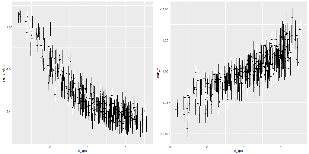
One interesting feature of the previous two graphs is the rather obvious systematic trend with radius of both SFR density and specific star formation rate, as shown more directly below taken from the first set of model runs:

sfr_ssfr_d_8479-12701
NGC 4889 (MaNGA plateifu 8479-12701) ΣSFR and SSFR vs. distance from IFU center

Are these real trends? I don’t know, but I don’t see an obvious reason why they might be spurious features of the models. In normal star forming galaxies I encounter trends with radius in both directions and sometimes no trend at all.

As a final and related aside there was a paper by Sedgwick et al. that showed up on arxiv not long ago that presented estimates of star formation rates of early type galaxies from observations of core collapse supernovae carefully matched to host galaxies with high confidence morphological classifications. To oversimplify their conclusions they found that typically massive ellipticals might have specific star formation rates ∼ 10-11 / yr, which is somewhat higher than usually supposed. As I mentioned in my last post my models will always have some contribution from young stars and I typically get central estimates of SSFR > ∼ 10-11.5 even in galaxies with no hint of emission (as is the case with this Coma sample). This particular galaxy has a total stellar mass within the IFU of ∼ 1011.5 M , so it could be forming stars at a rate of ∼ 1 M / yr.

Well, I think I have one more post to write before the SDSS DR17 release.

A little more on nonparametric line of sight velocity distribution modeling – is regularization needed?

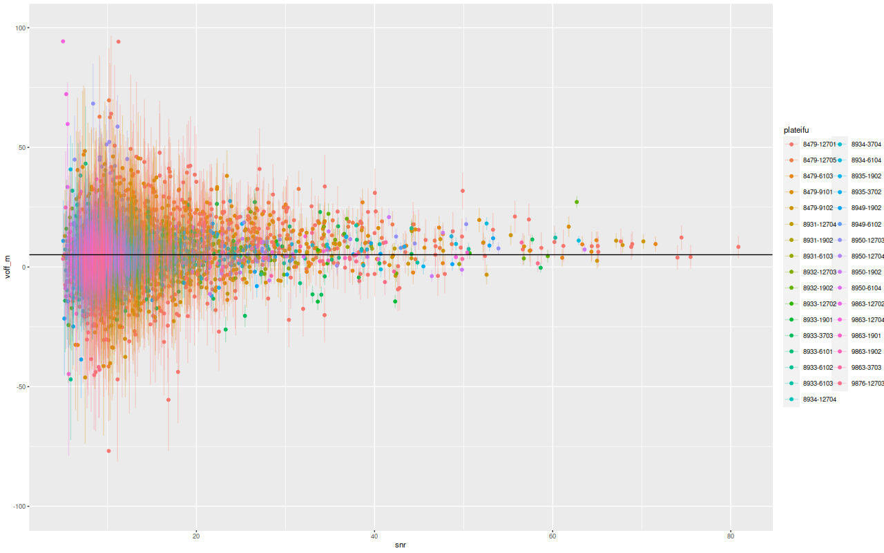
A while back I completed LOSVD models for 3348 spectra in the 33 Coma Cluster galaxies I chose for an initial sample. I want to look briefly at a couple summary statistics from the models. For each sample in the posterior I calculate first and second moments of the velocity distribution, and from those I calculate means and standard deviations of velocity offsets and velocity dispersions. Recall from the earlier posts that wavelengths are in the spectrum rest frame with peculiar velocities estimated by fitting a set of eigenspectra to the data. The first plot below is the mean velocity offset with errorbars ± 1 standard deviation versus the signal to noise in each spectrum. The horizontal line is the overall median of 5.25 km/sec. This is less than 1/10th the width of a wavelength bin and, I think, consistent with the absolute wavelength calibration accuracy claimed by the MaNGA team. From an eyeball analysis there doesn’t appear to be any trend in the mean with S/N, but the dispersion in estimates increases as the data quality gets worse. This seems unlikely to be a real problem. Two outliers cut off from the graph had mean velocity offsets of ≈ 200 km/sec, which is only 3 wavelength bins.

voff_v_snr
Mean velocity offset and standard deviation of mean vs. spectrum S/N for 33 passively evolving Coma Cluster galaxies. Solid horizontal line is median offset.

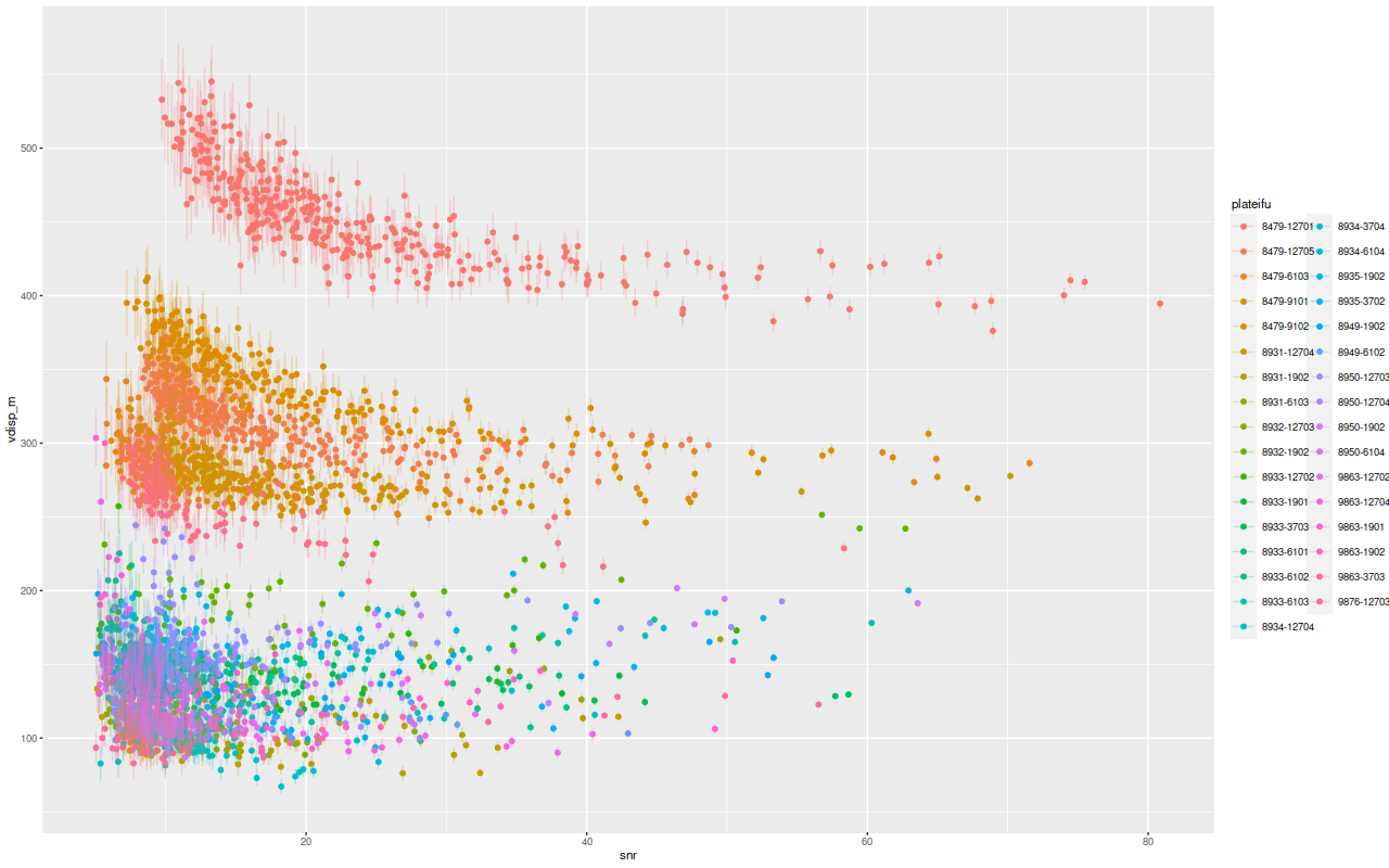
Possibly more concerning is that the mean velocity dispersion also shows a systematic trend with S/N:

vdisp_v_snr
Mean velocity dispersion and standard deviation of mean vs. spectrum S/N for 33 passively evolving Coma Cluster galaxies.

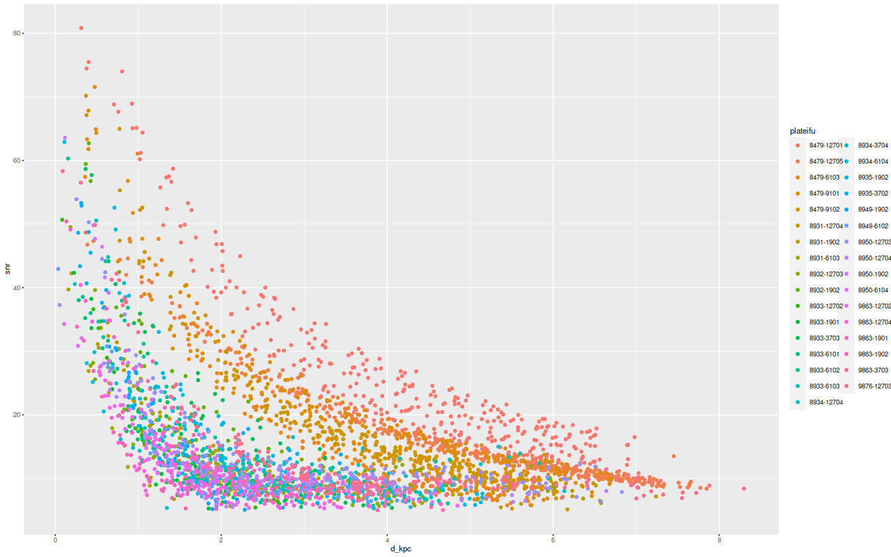
Of course there is a wide range of velocity dispersions since there’s a range of galaxy masses in this sample, but each galaxy shows a similar trend. This matters because, of course, S/N correlates strongly with distance from the nucleus which is usually the IFU center and this in turn leads to potentially spurious correlations with distance.

MaNGA spectrum S/N vs. distance from IFU center in kpc. — 33 passively evolving Coma Cluster galaxies

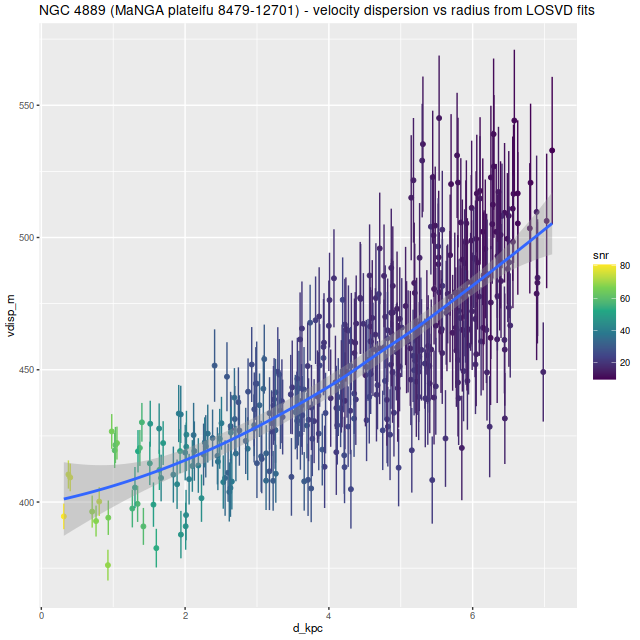
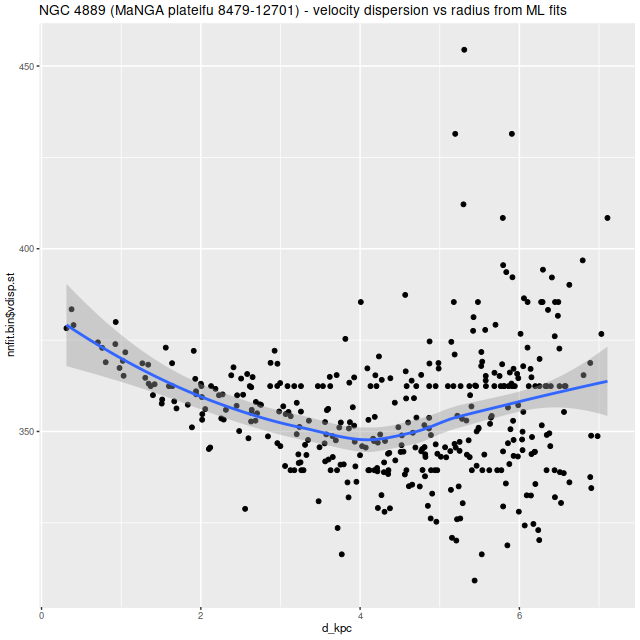
For example here are results for the cD galaxy NGC 4889 with MaNGA plateifu 8479-12701. This has the highest overall velocity dispersion in the sample by a fair margin as seen in the plots above. Plotting the estimated velocity dispersion against distance from the IFU center shows an apparent systematic increase1the trendline is just a “loess” smooth fit to mislead the eye and shouldn’t be interpreted as any kind of analysis:

NGC 4889 (MaNGA plateifu 8479-12701) – mean velocity dispersion vs. radius per nonparametric LOSVD fit.

Now this could be a real trend: my recollection is the outskirts of cD galaxies have essentially the velocity dispersion of the clusters they live in, which is taken as strong evidence that they grow by cannibalism. But the IFU only covers the inner part of this galaxy and in any case the confounding effect of the correlation between S/N and modeled velocity dispersion prevents any conclusion. Just for comparison here is the same relation using the single gaussian estimates from the preliminary maximum likelihood fits:

NGC 4889 (MaNGA plateifu 8479-12701) – velocity dispersion vs. radius per maximum likelihood fit.

So, if we’re interested in kinematics or dynamics some regularization with an informative prior seems advisable. What’s not so clear is whether this matters in SFH modeling, which as I’ve said many times is what most interests me. There’s one way to find out…

NGC 4949 – first attempt at modeling star formation histories with non-parametric losvd’s

I only have time to analyze one MaNGA galaxy for now and since it was the first to get the correctly coded LOSVD estimates I chose the Coma Cluster S0 galaxy NGC 4949 that I discussed in the last post for SFH modeling. As I mentioned a few posts ago trying to model the LOSVD and star formation history simultaneously is far too computationally intensive for my resources, so for now I just convolve the SSP model spectral templates with the elementwise means of the convolution kernels estimated as described previously and feed those to the SFH modeling code. My intuition is that the SFH estimates should be at least slightly more variable if the kinematics are treated as variable as well, but for now there’s no real alternative to just picking a fiducial value. Of course a limited test of that hypothesis could be made by pulling multiple draws from the posterior of the LOSVD distribution. I will certainly try that in the future.

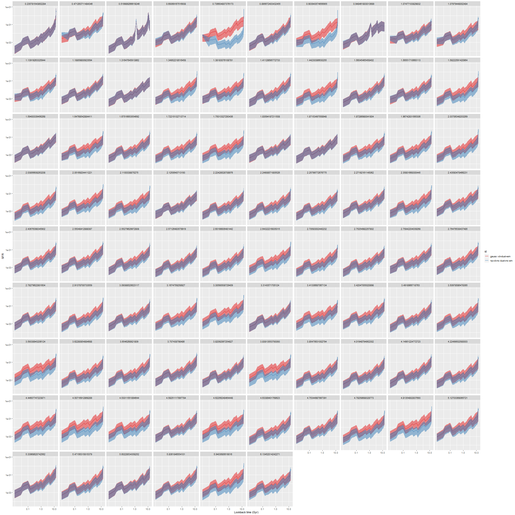
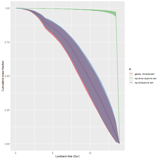
My first idea was to leave both dust and emission lines out of the SFH models. The first choice was to save CPU cycles and also based on the expectation that these passively evolving galaxies should have very little dust. The results were rather interesting: here are ribbon plots of model SFH’s for all 86 binned spectra. The pink ribbons are from the original model runs, which assumed single component gaussian velocity distributions, modified Calzetti attenuation, and included emission lines (which contribute negligible flux throughout). The blue ribbons are with non-parametric LOSVD and no attenuation model:

NGC 4949 – modeled star formation histories with single component gaussian and nonparametric estimates of line of sight velocity distributions with no dust model

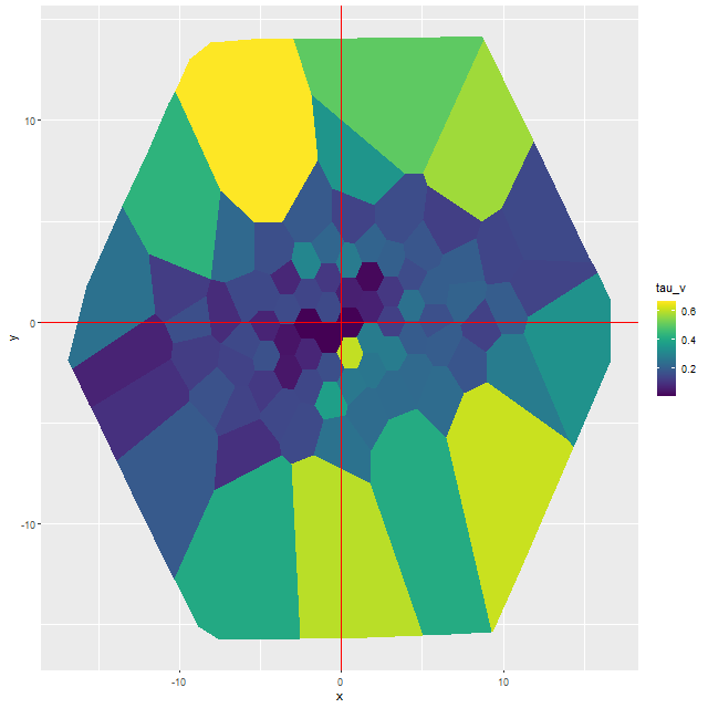
The differences in star formation histories turn out to be almost entirely due to neglecting dust in the second set of model runs. In this galaxy there are some areas with apparently non-negligible amounts of dust:

NGC 4949 – map of estimated optical depth of attenuation

Ignoring attenuation forces the model to use redder, hence older (and probably more metal rich although I haven’t yet checked) stellar populations and this has, in some cases, profound effects on the model SFH.

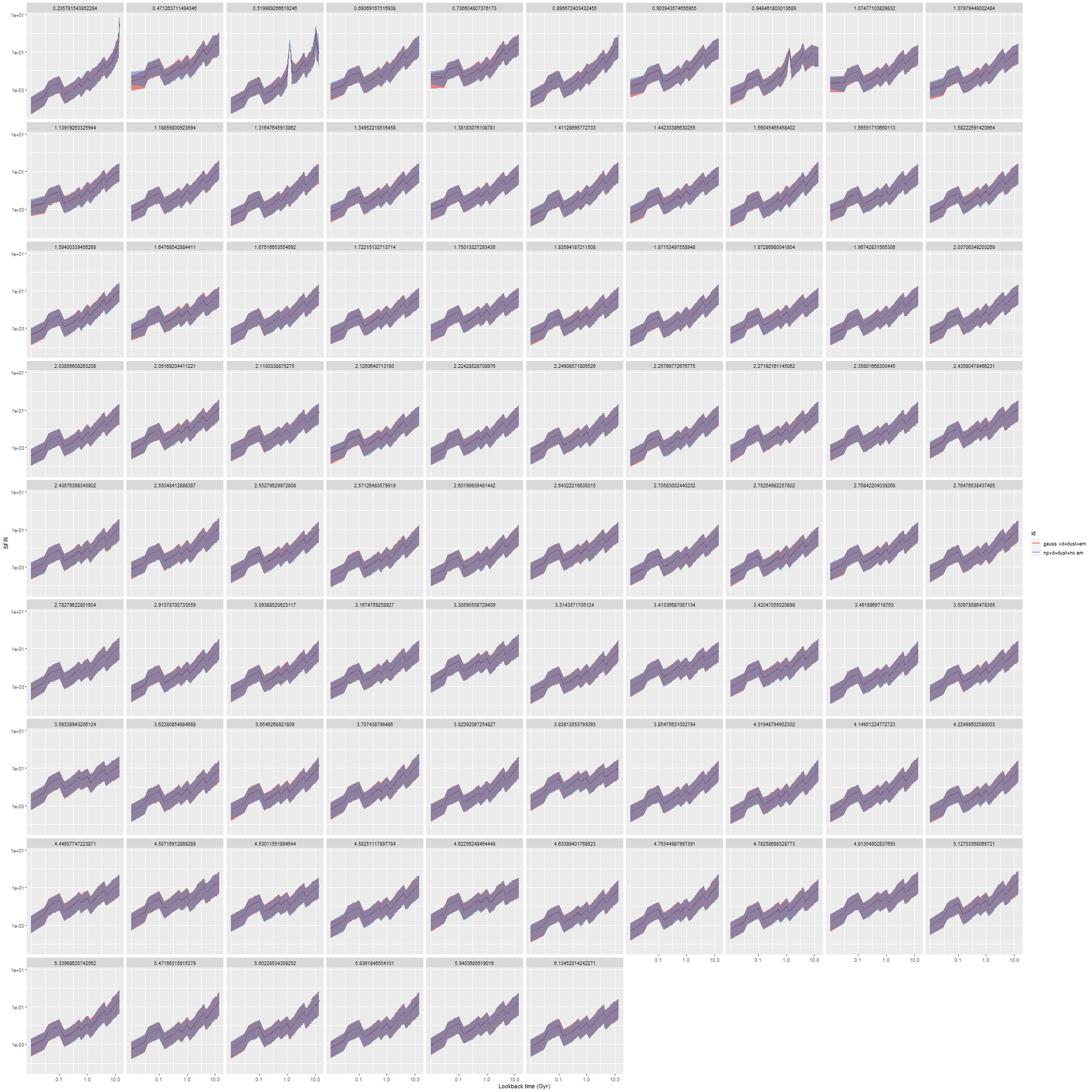
So, I tried a second set of model runs adding back in modified Calzetti attenuation but still leaving out emission:

ngc4949_sfh0_sfhnpvddust
NGC 4949 – modeled star formation histories with single component gaussian and nonparametric estimates of line of sight velocity distributions

And now the models are nearly identical, with minor differences mostly in the youngest age bin. All other quantities that I track are similarly nearly identical in both model runs.

Here is the modeled mass growth history for a single spectrum of a region just south of the nucleus that had the largest difference in model SFH in the second set of runs, and the largest optical depth of attenuation in the first and 3rd. This is an extreme case of the shift towards older populations required by the neglect of reddening. Well over 90% of the present day stellar mass was, according to the model, formed in the first half Gyr after the big bang with almost immediate and complete quenching thereafter. While not an impossible star formation history it’s not one I often see result from these models, which strongly favor more gradual mass buildup.

ngc4949_mgh3models_spec14
NGC 4949 – modeled mass growth histories for models with and without an attenuation model

So, the conclusion for now is that having an attenuation model matters a lot, the detailed stellar kinematics not so much. Of course this is a relatively simple example because it’s a rapid rotator and the model convolution kernels are fairly symmetrical throughout the galaxy. The massive ellipticals and especially cD galaxies with more complex kinematics might provide some surprises.

Update on Bayesian line of sight velocity modeling

Well that was simple enough. I made a simple indexing error in the R data preprocessing code that resulted in a one pixel offset between the template and galaxy spectra, which effectively resulted in shifting the elements of the convolution kernel by one bin. I had wanted to look at a rotating galaxy to perform some diagnostic tests, but once I figured out my error this turned out to be a pretty good validation exercise. So I decided to make a new post. The galaxy I’m looking at is NGC 4949, another member of the sample of passively evolving Coma cluster galaxies of Smith et al. It appears to me to be an S0 and is a rapid rotator:

NGC 4949 – SDSS image
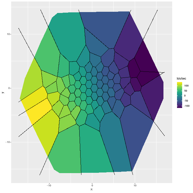
NGC 4949 – radial velocity map

These projected velocities are computed as part of my normal workflow. I may in a future post explain in more detail how they’re derived, but basically they are calculated by finding the best redshift offset from the system redshift (taken from the NSA catalog which is usually the SDSS spectroscopic redshift) to match the features of a linear combination of empirically derived eigenspectra to the given galaxy spectrum.

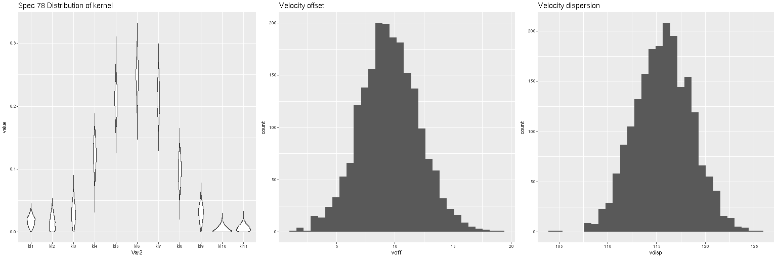
First exercise: find the line of sight velocity distribution after adjusting to the rest frame in each spectrum. This was the originally intended use of these models. This galaxy has fairly low velocity dispersion of ~100 km/sec. so I used a convolution kernel size of just 11 elements with 6 eigenspectra in each fit. Here is a summary of the LOSVD distribution for the central spectrum. This is much better. The kernel estimates are symmetrical and peak on average at the central element. The mean velocity offset is ≈ 9.5 km/sec, which is much closer to 0 than in the previous runs. I will look briefly at velocity dispersions at the end of the post: this one is actually quite close to the one I estimate with a single component gaussian fit (116 km/sec vs 110).

Estimated LOSVD of central spectrum of NGC 4949

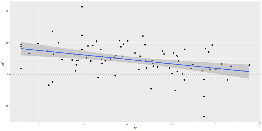
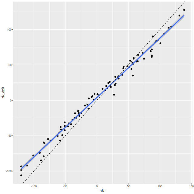
Next, here are the posterior mean velocity offsets for all 86 spectra in the Voronoi binned data, plotted against the peculiar velocity calculated as outlined above. The overall average of the mean velocity offsets is 4.6 km/sec. The reason for the apparent tilt in the relationship still needs investigation.
Mean velocity offset vs. peculiar velocity. All NGC 4949 spectra.

Exercise 2: calculate the LOSVD with wavelengths adjusted to the overall system redshift as taken from the NSA catalog, that is no adjustment is made for peculiar redshifts due to rotation. For this exercise I increased the kernel size to 17 elements. This is actually a little more than needed since the projected rotation velocities range over ≈ ± 100 km/sec. First, here is the radial velocity map:

Radial velocity map from Bayesian LOSVD model with no peculiar redshifts assigned.

Here’s a scatterplot of the velocity offsets against peculiar velocities from my normal workflow. Again there’s a slight tilt away from a slope of 1 evident. The residual standard error around the simple regression line is 6.4 km/sec and the intercept is 4 km/sec, which are consistent with the results from the first set of LOSVD models.

Velocity offsets from Bayesian LOSVD models vs. peculiar velocities

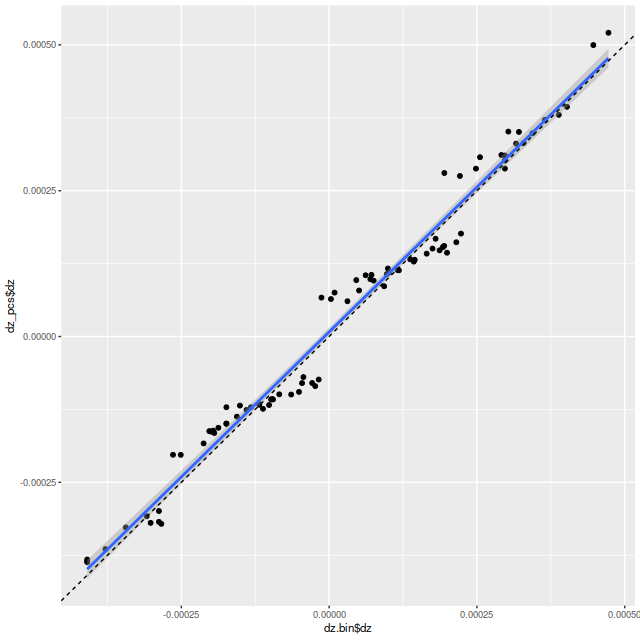
Exercise 3: calculate redshift offsets using a set of (for this exercise, 6) eigenspectra from the SSP templates. Here is a scatterplot of the results plotted against the redshift offsets from my usual empirically derived eigenspectra. Why the odd little jumps? I’m not completely sure, but my current code does an initial grid search to try to isolate the global maximum likelihood, which is then found with a general purpose nonlinear minimizer. The default grid size is 10-4, about the size of the gaps. Perhaps it’s time to revisit my search strategy.

Redshift offsets from a set of SSP derived eigenspectra vs. the same routine using my usual set of empirically derived eigenspectra.

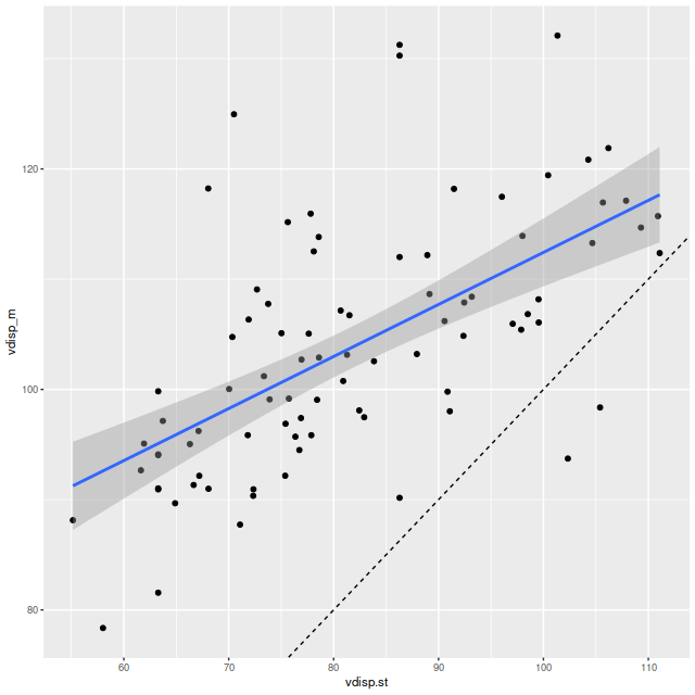
Final topic for now: I mentioned in the last post that posterior velocity dispersions (measured by the standard deviation of the LOSVD) were only weakly correlated with the stellar velocity dispersions that I calculate as part of my standard workflow. With the correction to my code the correlation while still weak has greatly improved, but the dispersions are generally higher:

Velocity dispersion form Bayesian LOSVD models vs. stellar velocity dispersion from maximum likelihood fits.

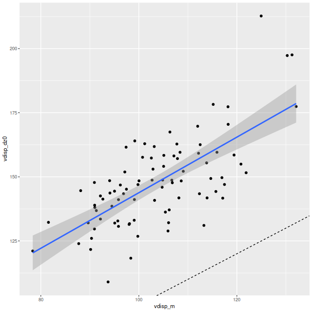
A similar trend is seen when I plot the velocity dispersions from the LOSVD models with correction only for the system redshift and a wider convolution kernel (exercise 2 above) with the fully corrected model runs (exercise 1):

These results hint that the diffuse prior on the convolution kernel is responsible for the different results. As part of the maximum likelihood fitting process I estimate the standard deviation of the stellar velocity distribution assuming it to be a single component gaussian. While the distribution of kernel values in the first graph look pretty symmetrical the tails are on average heavier than a gaussian. This can be seen too in the LOSVD models with the larger convolution kernel of exercise 2. The tails have non-negligible values all the way out to the ends:

Now, what I’m really interested in are model star formation histories. I’ve been using pre-convolved SSP model templates from the beginning along with phony emission line spectra with gaussian profiles with some apparent success. My plan right now is to continue that program with these non-parametric LOSVD’s. The convolutions could be carried out with posterior means of the kernel values or by drawing samples. Repeated runs could be used to estimate how much variation is affected by uncertainty in the kernel.

How to handle emission lines is another problem. For now stepping back to a simpler model (no emission, no dust) would be reasonable for this Coma sample.
Arxiv notes: “BAYES-LOSVD: a bayesian framework for … line-of sight velocity distributions”

This paper by J. Falcón-Barroso and M. Martig that showed up on arxiv back in November interested me for a couple reasons. First, this was one of the first research papers I’ve seen to make use of the Stan language or indeed any implementation of Hamiltonian Monte Carlo. What was even more interesting was they were doing exactly something I experimented with a few years ago, namely estimating the elements of convolution kernels for non-parametric description of galaxy stellar kinematics. And in fact their Stan code posted on github has comment lines linking to a thread on discourse.mc-stan.org I initiated where I asked about doing discrete convolution by direct multiplication and summation.
The idea I was pursuing at the time was to use sets of eigenspectra from a principal components decomposition of SSP model spectra as the bases for fitting convolved model spectra, with the expectation being that considerable dimensionality reduction could be achieved by using just the leading PC’s, which would in turn speed up model fitting. In fact this was certainly the case, although at the time I perhaps overestimated the number of components needed 1I mentioned in that thread that by one criterion — now forgotten — I would need 42, which is about an 80% reduction from the 216 spectra in the EMILES subset I use but still more than I expected. and I found the execution time to be disappointingly large. Another thing I had in mind was that I wanted to constrain emission line kinematics as well, and I couldn’t quite see how to do that in the same modeling framework. So, I soon turned away from this approach and instead tried to constrain both kinematics and star formation histories using the full SSP library and what I dubbed a partially parametric approach to kinematic modeling, using a convolution kernel for the stellar component and Gauss-Hermite polynomials for emission lines. This works, more or less, but it’s prohibitively computationally intensive, taking an order of magnitude or more longer to run than the models with preconvolved spectral templates. Consequently I’ve run this model fewer than a handful of times and only on a small number of spectra with complicated kinematics.

Falcón-Barroso and Martig started with exactly the same idea that I was pursuing of radically reducing the dimensionality of input spectral templates through the use of principal components. They added a few refinements to their models. They include additive Legendre polynomials in their spectral fits, and they also “regularize” the convolution kernels with informative priors of various kinds. Adding polynomials is fairly common in the spectrum fitting industry, although I haven’t tried it myself. There is only a short segment in the red that is sometimes poorly fit with the EMILES library, and that would seem to be difficult to correct with low order polynomials. What does affect the continuum over the entire wavelength range and could potentially cause a severe template matching issue is dust reddening, and this would seem to be more suitable for correction with multiplicative polynomials or simply with the modified Calzetti relation that I’ve been using for some time.

I’m also a little ambivalent about regularizing the convolution kernel. I’m mostly interested in the kinematics for the sake of matching the effective SSP model spectral resolution to that of the spectra being modeled for star formation histores, and not so much in the kinematics as such.

I decided to take another look at my old code, which somewhat to my surprise I couldn’t find stored locally. Fortunately I had posted the complete code on that discourse.mc-stan thread, so I just copied it from there and made a few small modifications. I want to keep things simple for now, so I did not add any polynomial or attenuation corrections and I am not trying to model emission lines. I also didn’t incorporate priors to regularize the elements of the convolution kernel. Without an explicit prior there will be an implicit one of a maximally diffuse dirichlet. I happen to have a sample of MaNGA spectra that are well suited for a simple kinematic analysis — 33 Coma cluster galaxies from a sample of Smith, Lucey, and Carter (2012) that were selected to be passively evolving based on weak Hα emission, which virtually guarantees overall weak emission. Passively evolving early type galaxies also tend to be nearly dust free, making it reasonable not to model it.

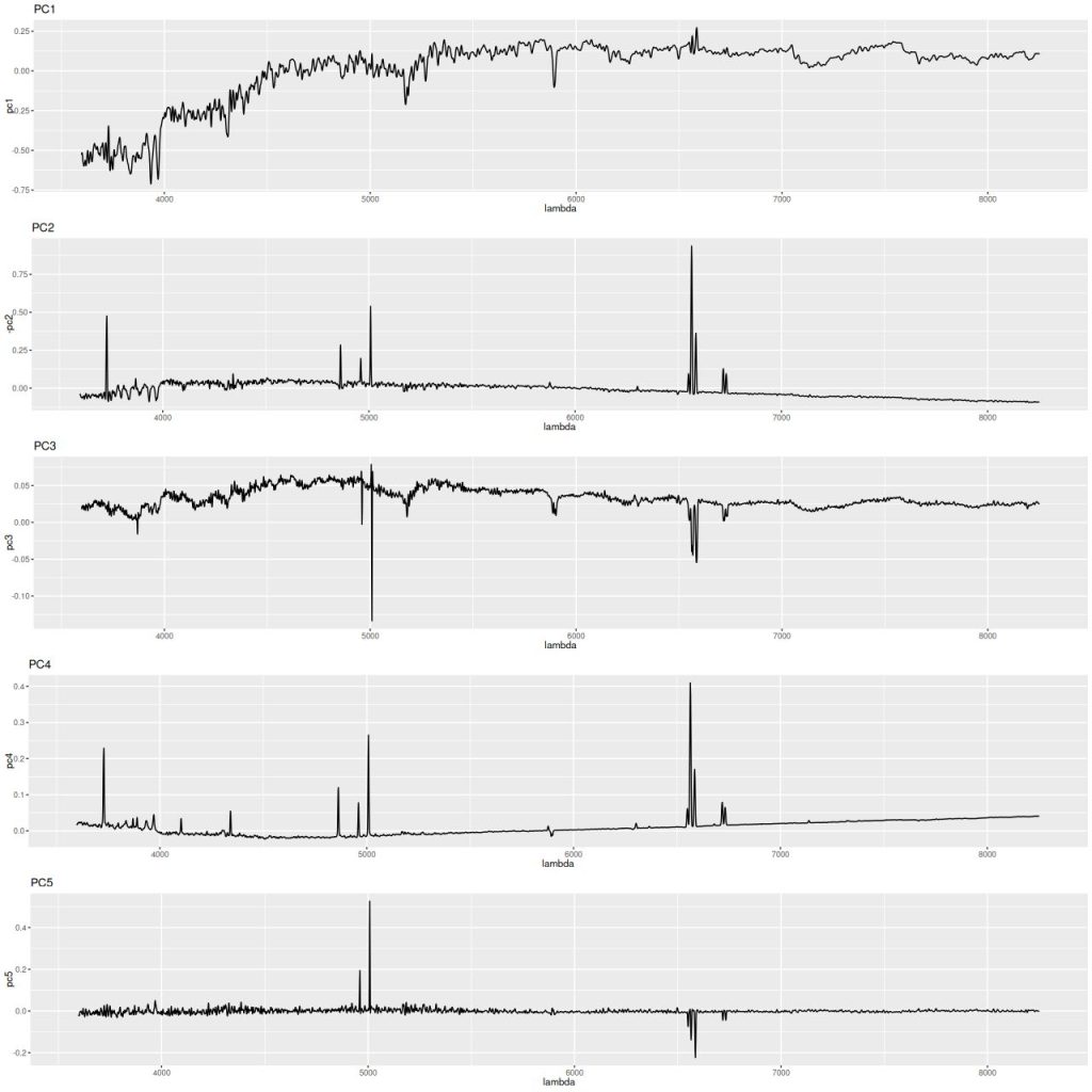
I’ve already run SFH models for all of these galaxies, so for each spectrum in a galaxy I adjust the wavelengths to rest frame using the system redshift and redshift offsets that were calculated in the previous round. I then regrid the SSP library (as usual the 216 component EMILES subset) templates to the galaxy rest frame and extract the region where there is coverage of both the galaxy spectrum and the templates. I then standardize the spectra (that is subtract the means and divide by the standard deviations) and calculate the principal components using R’s svd() function. I again rescale the eigenvectors to unit variance and select the number I want to use in the models. I initially did this by choosing a threshold for the cumulative sum of the eigenvalues as a fraction of the sum of all. I think instead I should use the square of the eigenvalues since that will make the choice based on the fraction of variance in the selected eigenvectors. With the former criterion a threshold of 0.95 will result in selecting 8 eigenspectra, 0.975 results in 13 (perhaps ± 1). In fact as few as 2 or 3 might be adequate as noted by Falcón-Barroso and Martig. The picture below of three eigenspectra from one model run illustrates why. The first two look remarkably like real galaxy spectra, with the first looking like that of an old passively evolving population, while the second has very prominent Balmer absorption lines and a bluer continuum characteristic of a younger population. After that the eigenspectra become increasingly un-spectrum like, although familiar features are still recognizable but often with sign flips.

three_eigenspectra
First three eigenspectra from a principal components decomposition of an SSP model spectrum library

The number of elements in the convolution kernel is also chosen at run time. With logarithmic wavelength binning each wavelength bin has constant velocity width — for SDSS and MaNGA spectra of 69.1 km/sec. If a typical galaxy has velocity dispersion around 150 km/sec. and we want the kernel to be ≈ ±3 σ wide then we need 13 elements, which I chose as the default. Keep in mind that I’ve already estimated redshift offsets from the system value for each spectrum, so a priori I expected the mean velocity to be near 0. If peculiar velocities have to be estimated the convolution kernel would need to be much larger. Also in giant ellipticals and other fairly rare cases the velocity dispersion could be much larger as we’ll see below.

Lets look at a few examples. I’ve only run models so far for three galaxies with a total of 434 spectra. One of these (SDSS J125643.51+270205.1) appears disky and is a rapid rotator. The most interesting kinematically is NGC 4889, a cD galaxy at the center of the cluster. The third is SDSS J125831.59+274024.5, a fairly typical elliptical and slow rotator. These plots contain 3 panels. The left shows the marginal posterior distribution of the convolution kernels, displayed as “violin” plots. The second and third are histograms of the mean and standard deviation of the velocities. For now I’m just going to show results for the central spectrum in each galaxy. These are fairly representative although the distributions in each velocity bin get more diffuse farther out as the signal/noise of the spectra decrease. I set the kernel size to the default for the two lower mass galaxies. The cD has much higher velocity dispersion of as much as ~450 km/sec within the area of the IFU, so I selected a kernel size of 39 (± 1320 km/sec) for those model runs. The kernel appears to be fairly symmetrical for the rotating galaxy (top panes), while the two ellipticals show some evidence of multiple kinematic components. Whether these are real or statistical noise remains to be seen.

centrallosvd_8931_1902
Distribution of kernel, velocity offset, and velocity dispersion. Central spectrum of MaNGA plateifu 8931-1902
centrallosvd_8933_6101
Distribution of kernel, velocity offset, and velocity dispersion. Central spectrum of MaNGA plateifu 8933-6101
centrallosvd_8479_12701
Distribution of kernel, velocity offset, and velocity dispersion. Central MaNGA spectrum of NGC 4889 (plateifu 8479-12701)

There are a couple surprises: the velocity dispersions summarized as the standard deviations of the weighted velocities are at best weakly correlated and generally larger than the values estimated in the preliminary fits that I perform as part of the SFH modeling process. More concerning perhaps is the mean velocity offset averages around -50 km/sec. This is fairly consistent across all three galaxies examined so far. Although this is less than one wavelength bin it is larger than the estimated uncertainties and therefore needs explanation.

hist_velocity_offset
Distribution of mean velocity offsets from estimated redshifts for 434 spectra in 3 MaNGA galaxies.

Some tasks ahead: Figure out this systematic. Look at regularization of the kernel. Run models for the remaining 30 galaxies in the sample. Look at the effect on SFH models.