I’ve written a few times about my dissatisfaction with the EMILES based SSP model library that I’ve used for star formation history modeling for some years and my desultory search for a replacement: This post from early 2024 was the most detailed. Unfortunately neither of the two alternatives I tested were quite satisfactory and my hopes for a MaStar based library from the final MaNGA data release haven’t yet materialized nearly a year later. I’ve given some thought to producing my own but I don’t know exactly how to create sets of summed spectra from a collection of isochrones and given IMF, and it wasn’t really something I wanted to learn. It’s also the case that even though MaStar has many more stellar spectra than any other publicly available collection (MILES, which is the basis for most (semi-)empirical libraries contains just 985) it still doesn’t fully span the space of physical parameters, so additional theoretical or empirical inputs will be required.
Somewhat serendipitously since I was traveling at the time and could easily have missed them a pair of papers appeared on arxiv on 23 October describing an R package named “ProGeny” that does precisely what I need: 2410.17697 and 2410.17698 by A. Robotham and S. Bellstedt. The first paper introduces the package and describes the data currently available for generating what they call Stellar Population Libraries (SPL). While it might seem surprising they used R for this1Python is the language of choice for most astronomers these days. the senior author has published several R packages for various astronomy related tasks, so it isn’t actually surprising that given their apparent need for this tool they chose R to implement it. This was a timely publication for me since I’ve about reached the limit of what I want to do with the EMILES library.
Besides the software which is written entirely in R, the authors did a good job of collating the publicly available data for the required inputs of isochrones and stellar atmospheres and packaging them into FITS files that are readable in R with the help of addon packages. Functions within ProGeny take care of reading the files and creating R objects for further processing.
After installing the software and dependencies and downloading the data files (several GB unzipped) I spent a little time browsing the (rather sparse) documentation and the two vignettes that have been published so far and it was then pretty straightforward to create a library with the recommended inputs. Specifically I used the MIST isochrones combined with the following stellar atmospheres: “C3K” for the base, “PHOENIX” extended, “AGB” from Lancon, “TMAP” for hot stars including remnants: see Table 3 of the first paper for descriptions and references. I used a Kroupa IMF with lower and upper mass limits of 0.1 and 100 M☉, which are fairly standard choices and the same as my EMILES based library. The constructed library has 107 age bins in logarithmic intervals of 0.05 dex ranging from log(T) = 5.0 to 10.3, 15 metallicity bins with log(Z/Z☉) ranging from -4 to +.5 with adopted Z☉ = 0.02, and wavelengths from 5.6 Å to 36 mm. Almost all of the data that I use as model inputs is calculated, including of course the spectra and remaining stellar mass at each age and metallicity. The only thing missing is relative g, r, i band fluxes that I use to calculate model intrinsic colors (something I occasionally look at as a sort of proxy for specific star formation rate). This I have existing code for.
These are more age/metallicity combinations than I need or probably can use and definitely a much larger wavelength range than needed for MaNGA data, so I’m experimenting with subsets. For a first pass I created a “small” subset with 42 ages ranging from log(T) = 6 to 10.1 in 0.1 dex increments and 5 metallicities log(Z/Z☉) = {-0.75, -0.25, 0, 0.25, 0.5}. The metallicity range is similar to my EMILES based library but with one more bin, while there are fewer but more evenly spaced age bins. I’ve also created a “large” subset with all 83 age bins between log(T) = 6 and 10.1, and the same 5 metallicities. I didn’t include younger populations for the simple reason that there’s not much evolution in the first Myr, which makes it difficult or impossible to disentangle their contributions. Similar considerations apply at the old end, and in addition there’s the fact that the current consensus age of the universe is 13.8 Gyr (log(T) = 10.14).
I’ve tentatively chosen a wavelength range of 3300-9000Å. The blue end was chosen to cover the shortest rest frame wavelength in MaNGA spectra for redshifts out to z ≈ 0.1. The red limit is more of a judgment call. Night sky lines become problematic at wavelengths as short as ≈ 8000Å, and in addition there’s an artifact called “blowtorch” by the SDSS team that causes an upturn at the very red end in some spectra. The chosen cutoff is just to the red of a set of Calcium triplet absorption lines at 8500-8700Å that are prominent in some spectra.
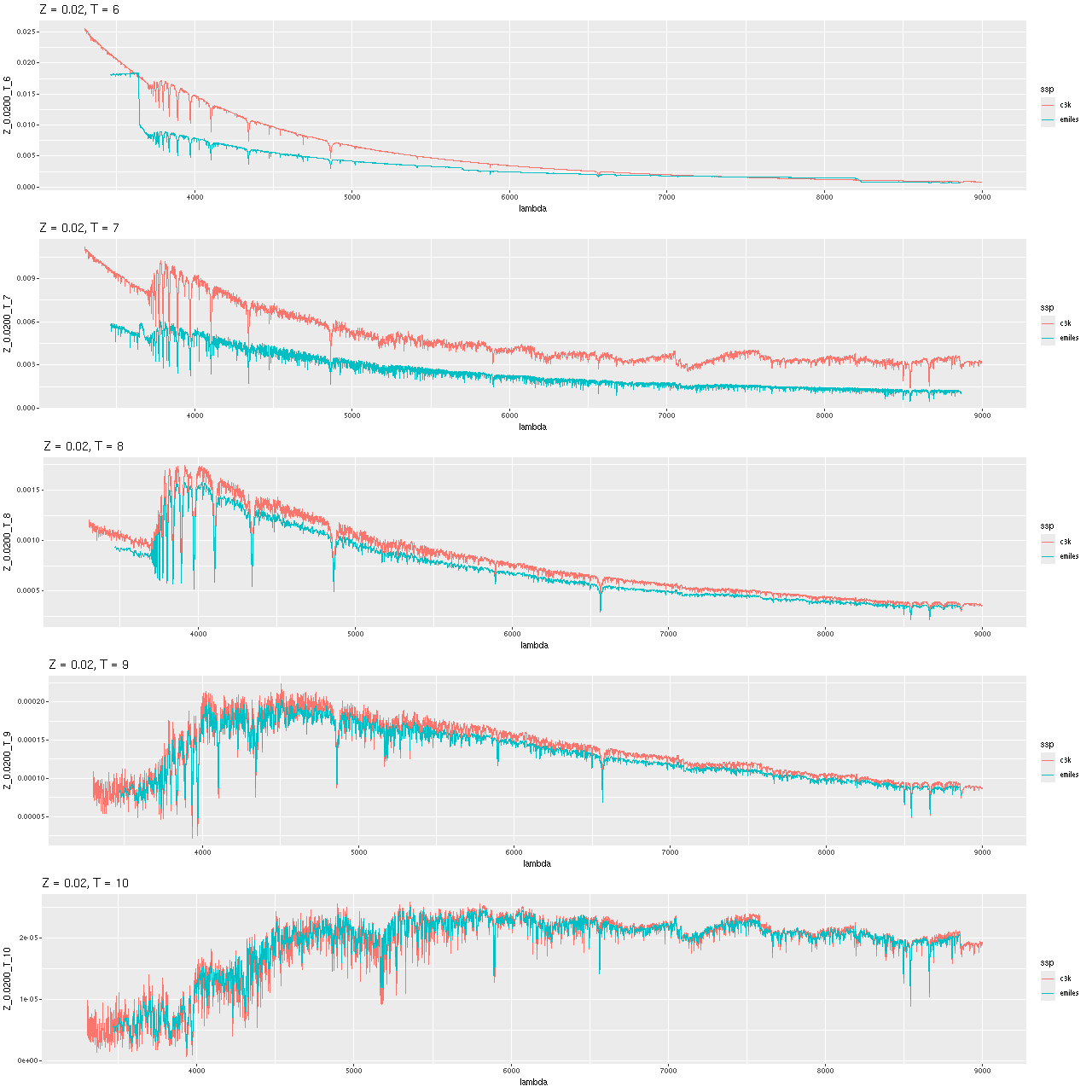
Below are comparisons of a few model spectra at solar metallicity and decade age intervals. Recall that the 106 and 107 year models are from the Hr-PyPopStar models of Millan-Irigoyen et al. (2021) including continuum emission. Evidently the newly constructed models are rather more luminous and bluer than the PyPopstar models, while closer to the EMILES models especially at ages > 1 Gyr. Possible differences in absorption line strengths could be due to finer wavelength sampling in the ProGeny models. One possibly significant difference is the MIST isochrones track more stages of stellar evolution than the version of BaSTI used for EMILES, including the asymptotic giant branch and stellar remnants. How much these contribute to the light in the relevant wavelength range and at what ages has yet to be investigated by me.
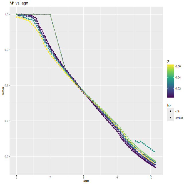
Modern collections of stellar isochrones generally include a prescription for mass loss and remnant masses in evolving populations. ProGeny calculates these and includes a data table of stellar masses in its SSP model output. The graph below compares the remaining stellar mass (including remnants) with age for the provisional library versus EMILES. I had assigned a relative stellar mass of 1 to the PyPopstar models, while the MIST isochrones indicate about a 10% mass loss by 107 years. At older ages the masses are very similar. This is much closer agreement than the equivalent graph in Figure 12 of paper 1, so the adopted relation shouldn’t be a source of significant differences in present day stellar mass computations.
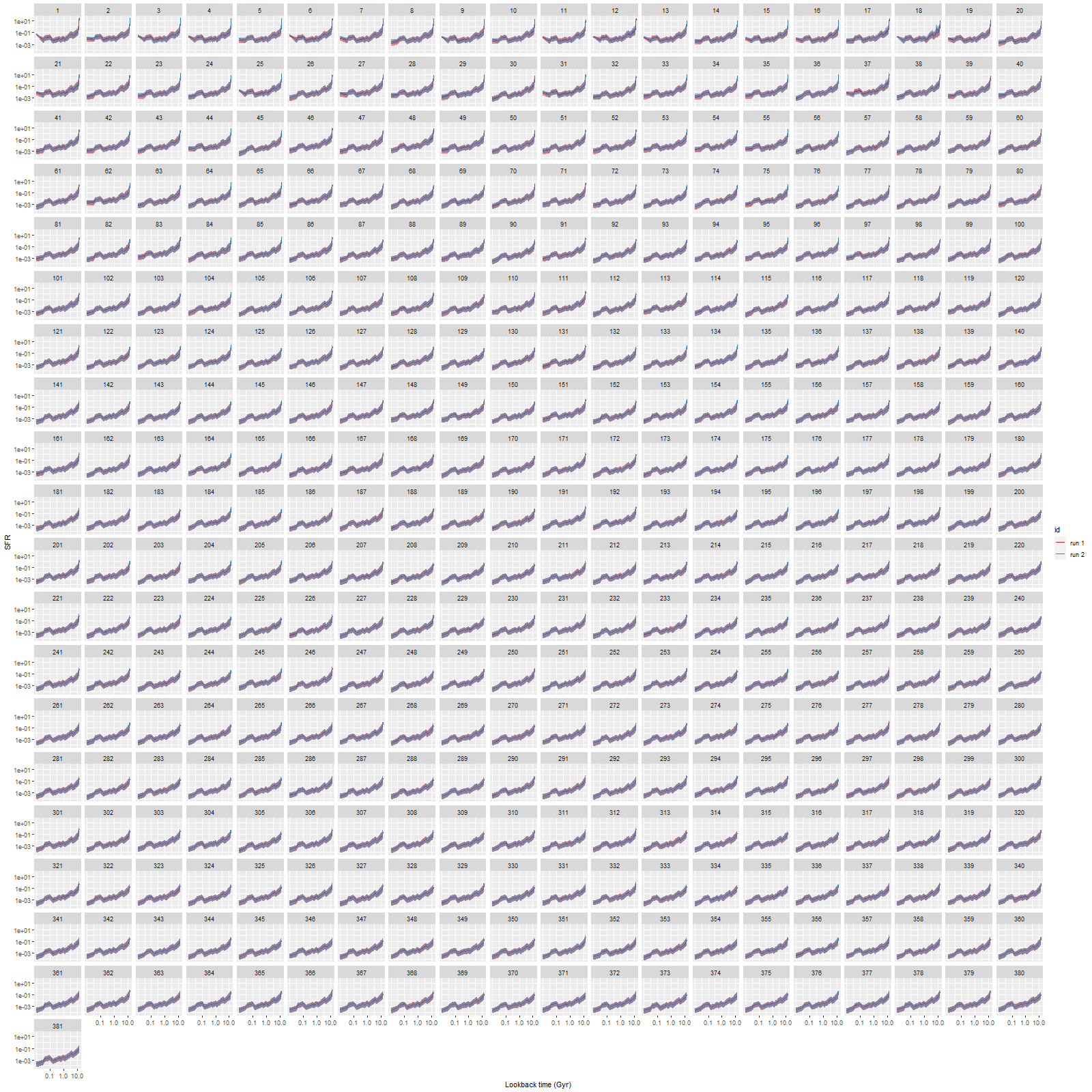
So far I’ve only run models for two galaxies with rather different properties, the same ones I wrote about in this post: the post-starburst plateifu 10220-3703 (mangaid 1-201936; NED name WISEA J080218.38+323207.8) and the late type spiral plateifu 11018-12704 (mangaid 1-233951; UGC 8162). Since it has taken much longer to prepare this post than I anticipated, I’m only going to discuss the post-starburst for now. The spiral will have to wait for the new year.
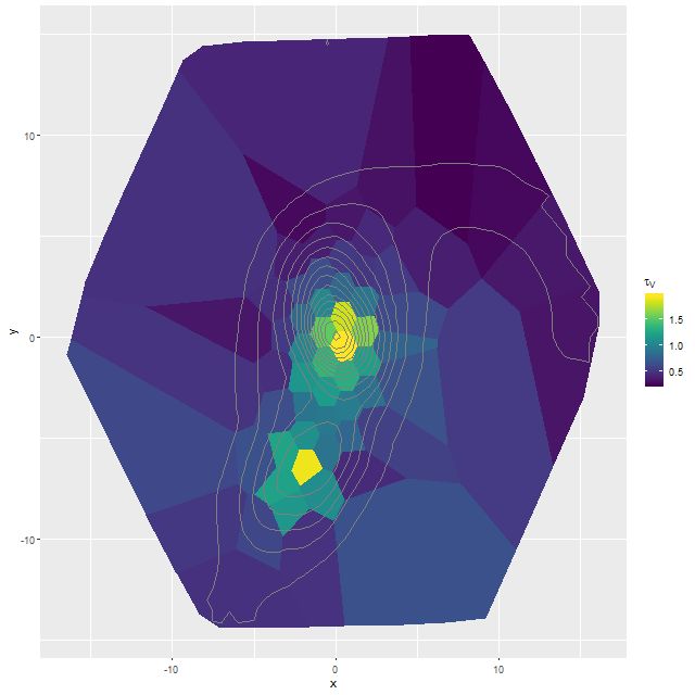
I did an initial set of runs with the same model formulation that I’ve used for a few years now and got some rather surprising results, particularly for outlying regions of the galaxy: model star formation histories looked more like an actively star forming galaxy than a passively evolving one, with younger populations and higher recent star formation rates. The models also had relatively high attenuation values with much steeper attenuation curves than are reported in the literature. This is I think a known “degeneracy” between attenuation and stellar age. The tentative solution was simply to tighten the priors on the two attenuation parameters: I set both upper and lower bounds on the steepness parameter δ: -0.5 < δ < 1.2 and also decreased the scale parameters on the priors for both τV and δ (see this post for my initial discussion of the attenuation model and the following one for problems I initially encountered; the parameterization was based on the work of Salim et al. 2018). Plugging into equation 4 of Salim et al. the limits on δ correspond to 1.6 < RV < 8.7, which is still a very large range.
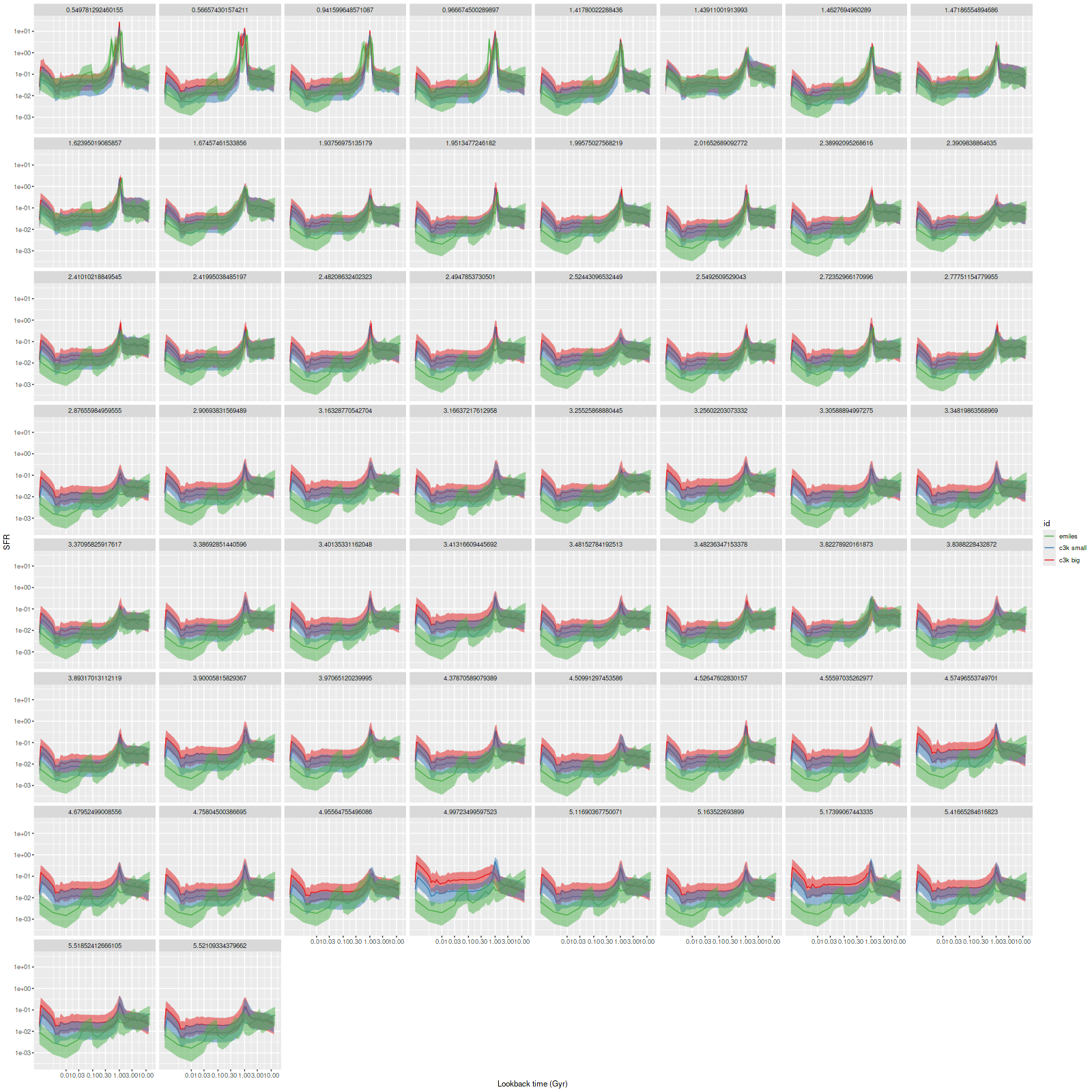
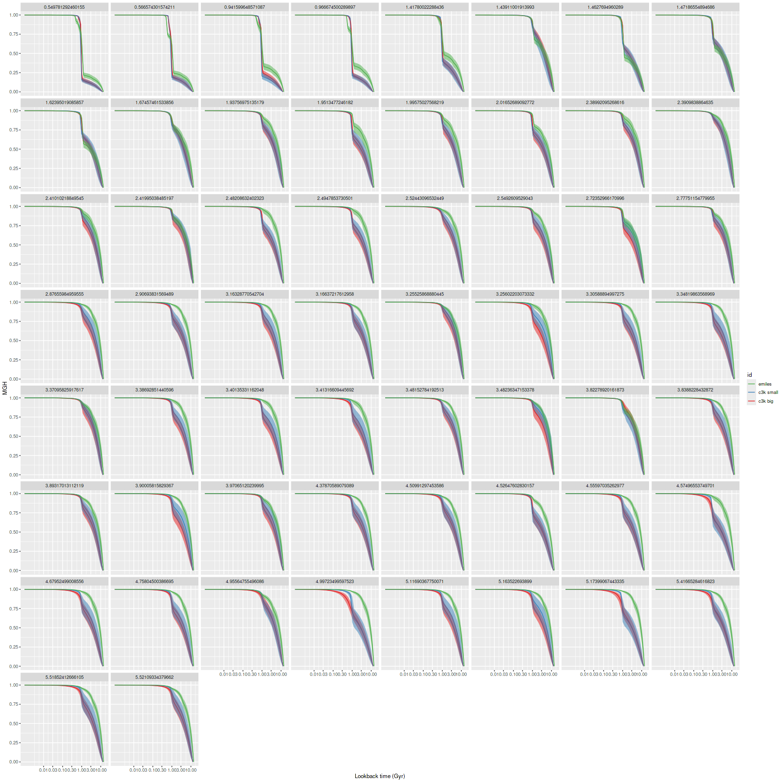
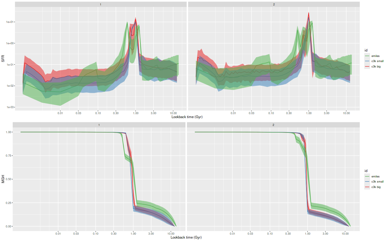
As can be seen from the SFH and mass growth plots below the C3K based models are fairly consistent with EMILES, although with generally higher late time star formation rates. Interestingly, the “big” models also have generally higher late time SFR than the “small” models even though they have the same stellar ingredients with just different time resolution. Both sets of models have gotten rid of the objectionable artificial jumps in star formation rates where the BaSTI models have abrupt changes in age intervals.
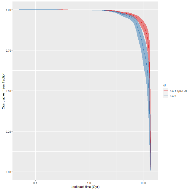
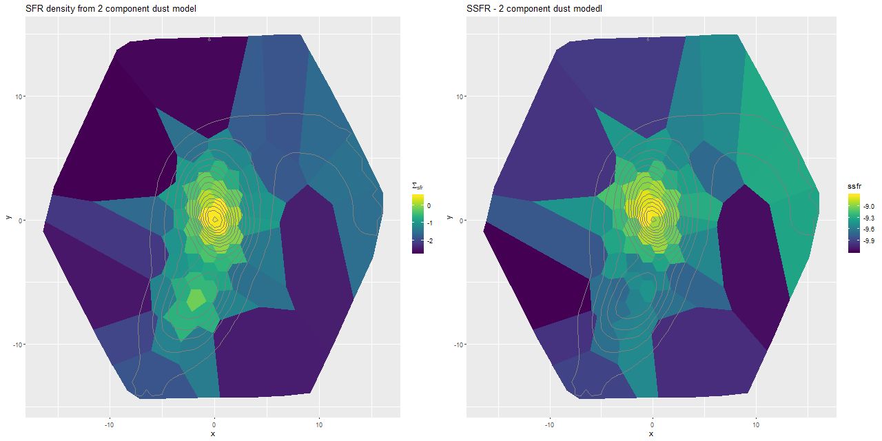
One fairly significant difference is that in the EMILES based models the burst appears to be strongly centrally concentrated, fading beyond about 2 kpc from the center. The C3K based models by contrast show a burst throughout. In the center the EMILES models have a complex, multipeaked evolution through the burst, while the C3K models have a fairly smooth rise and decline. Whatever hopes I had that it might be possible to time major events in possible merger scenarios seem to have been misguided., although the age and magnitude of the burst agree in all model runs.
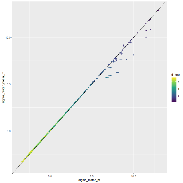
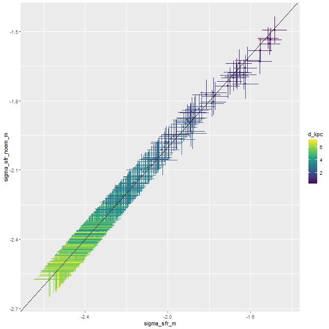
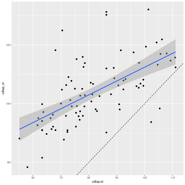
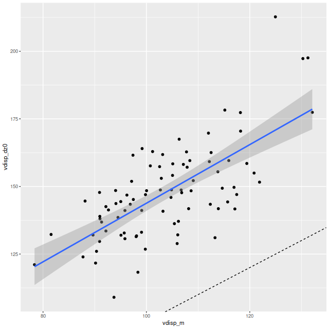
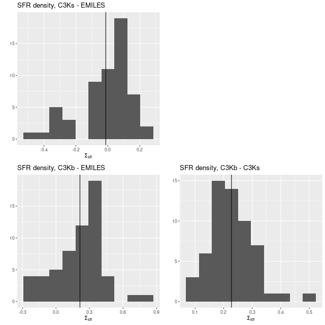
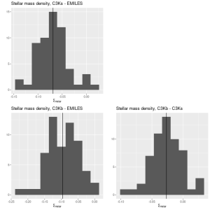
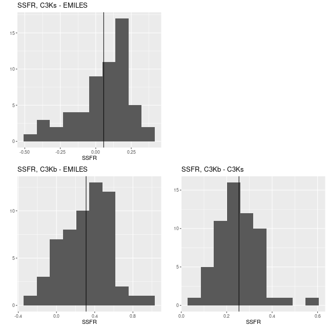
Here are pairwise differences in mean values between the models for some of the summary quantities I track. Some of the differences are fairly large, which just reinforces my longstanding opinion that true uncertainties are much larger than what’s captured in the posteriors of model runs.
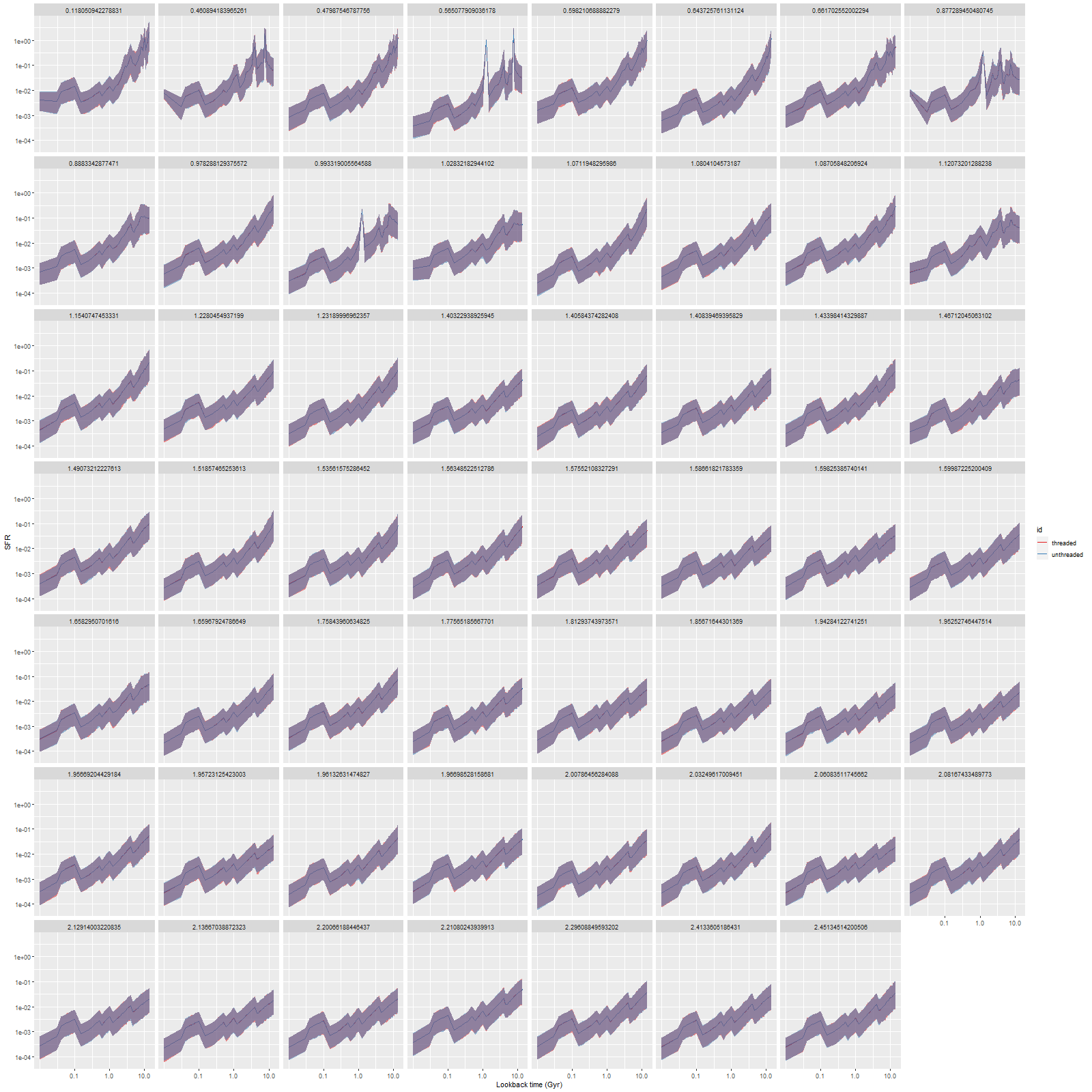
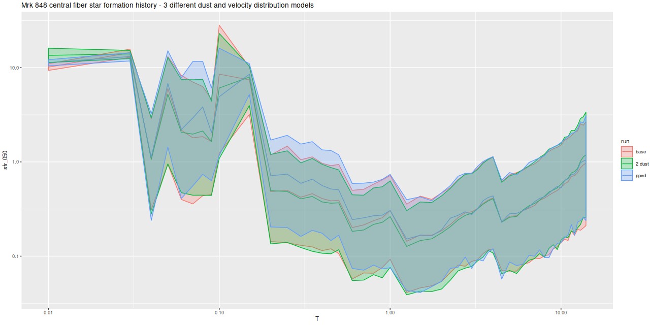
And finally, here is a closer look at star formation history models for the two fibers closest to the center:
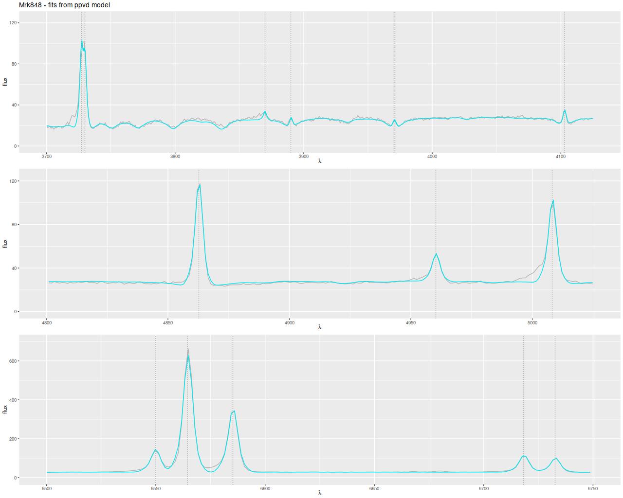
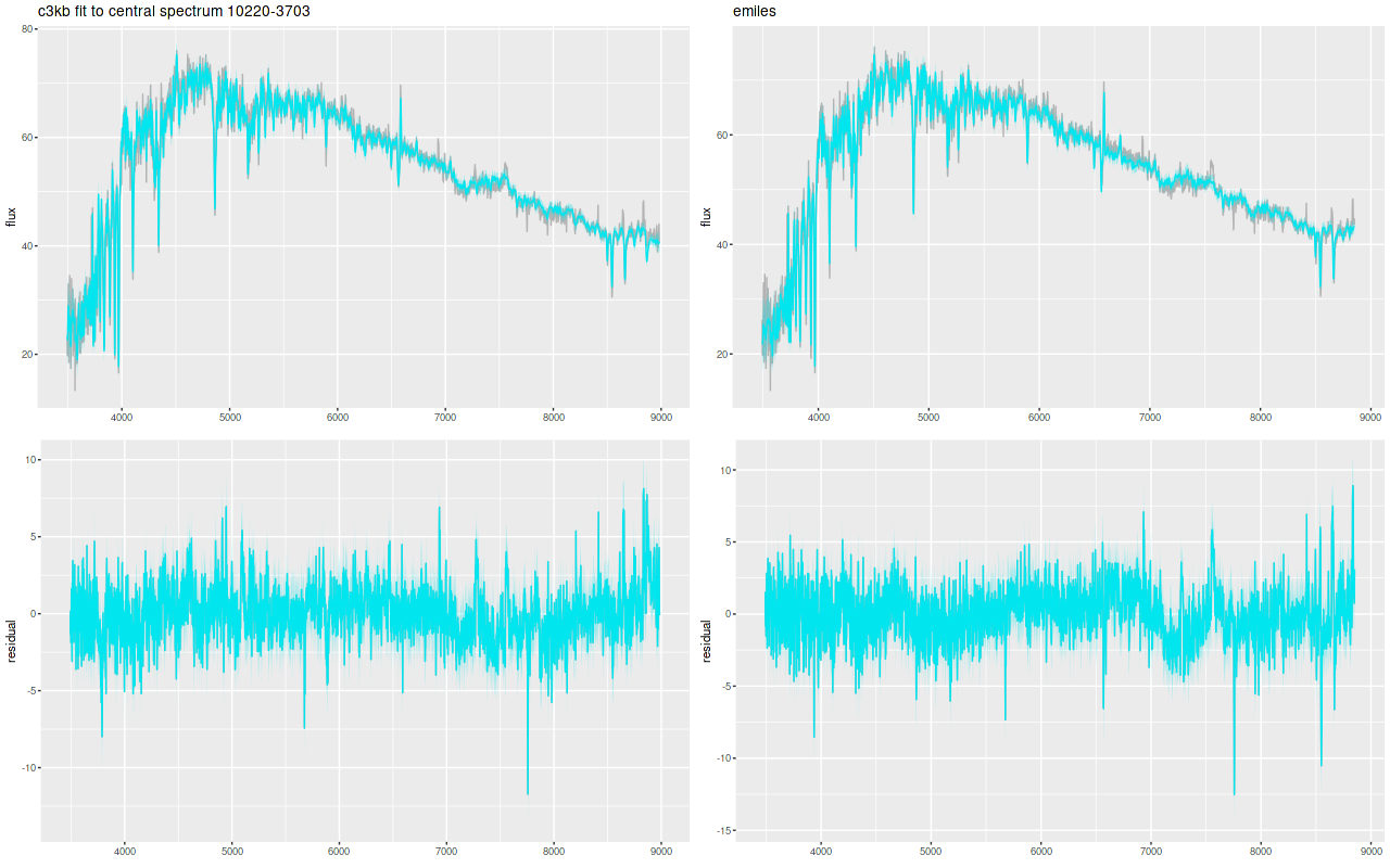
And here are (posterior predictive) fits to the data for the central spectrum with the large C3K based model (L) and EMILES (R). Both of these have some problematic areas, with some stretches of continuum and absorption line strengths “off” a bit. Note that the C3K model does better with the trough around 7200Å. The continuum upturn at the red end can also be seen in C3K model, which suggests I may want to consider truncating the model spectra a few hundred Ångstroms to the blue. Overall though fits to the data are very similar, and there’s little difference between the “large” and “small” C3K subsets.
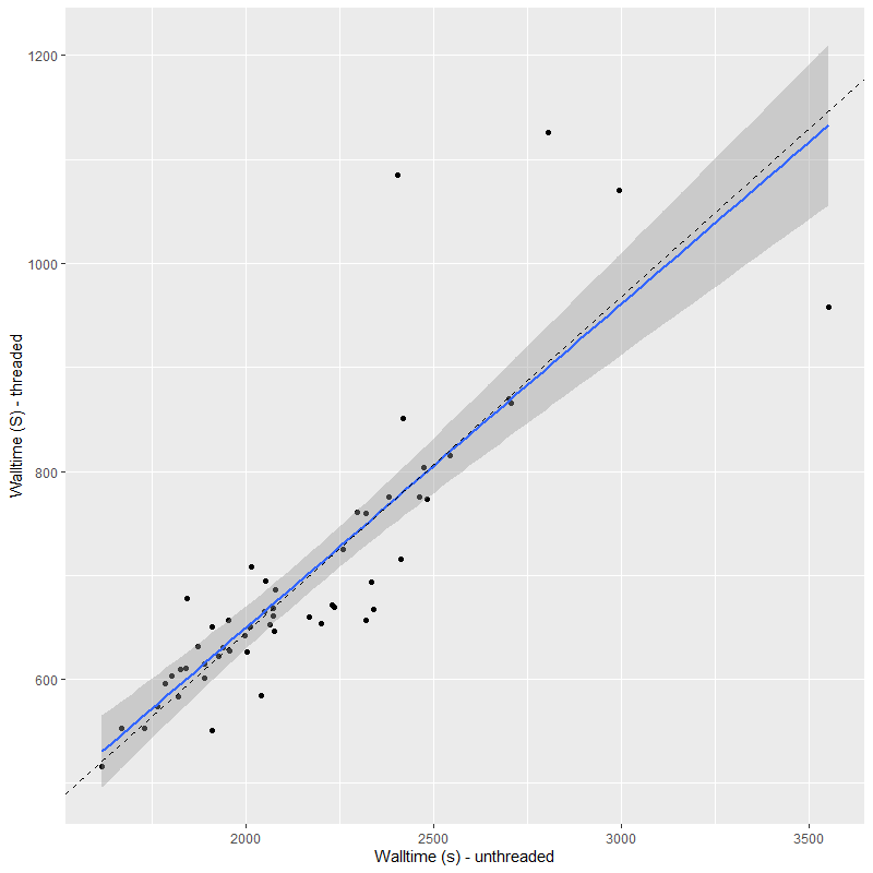
ProGeny is a useful tool and I hope the authors will be able to maintain it and add new capabilities and data sources. I still have a few things to do before resuming a modeling campaign: most importantly perhaps choosing a final subset of the full library, specifically the number of age and metallicity bins. The execution time of a model run is roughly proportional to the number of stellar contribution parameters. For this data set the average time with the EMILES library (224 SSP model spectra) was 618 sec, 576 sec for the small C3K library (210 spectra), and 1038 sec. for the large C3K library (415 spectra). That’s more time than I’d like to take. Would it be preferable to have a coarser metallicity grid, say log(Z/Z☉) = {-0.75, 0, 0.5} with the full 0.05 dex age spacing or a finer metallicity grid with 0.1 dex age bins? I don’t know: some fake data exercises might be appropriate at this point.
I still have some interest in using the MaStar spectra but there are some technical issues to solve. For one thing the data available on Skyserver are corrected to above the atmosphere but not for galactic extinction and are just apparent flux values rather than absolute ones. They also need to be reduced to rest frame wavelengths. ProGeny’s model spectra have a very wide wavelength range, which I assume is required to make the integrated model flux equal to the bolometric luminosity. Even though I don’t really need wavelengths outside the range of BOSS spectra I would need to extend them somehow anyway. Finally (?) the parameter coverage (temperature, gravity, metallicity) is still not quite complete, especially at for hot stars and very luminous ones so it would still be necessary to supplement the base library.