I’m stranded at sea at the moment so I may as well make a short post. First, here is the complete Stan code of the current model that I’m running. I haven’t gotten around to version controlling this yet or uploading a copy to my github account, so this is the only non-local copy for the moment.
One thing I mentioned in passing way back in this post is that making the stellar contribution parameter vector a simplex seemed to improve sampler performance both in terms of execution time and convergence diagnostics. This was for a toy model where the inputs were nonnegative and summed to one, but it turns out to work better with real data as well. At some point I may want to resurrect old code to document this more carefully, but the main thing I’ve noticed is that post-warmup execution time per sample is often dramatically faster than previously (the execution time for the same number of warmup iterations is about the same or larger though). This appears to be largely due to needing fewer “leapfrog” steps per iteration. It’s fairly common for a model run to have a few “divergent transitions,” which Stan’s developers seem to think is a strong indicator of model failure1I’ve rarely actually seen anything particularly odd about the locations of the divergences and inferences I care about seem unaffected. I’m seeing fewer of these and a larger percentage of model runs with no divergences at all, which indicates the geometry in the unconstrained space may be more favorable.
Here’s the Stan source:
// calzetti attenuation
// precomputed emission lines

functions {
  vector calzetti_mod(vector lambda, real tauv, real delta) {
    int nl = rows(lambda);
    real lt;
    vector[nl] fk;
    for (i in 1:nl) {
      lt = 5500./lambda[i];
      fk[i] = -0.10177 + 0.549882*lt + 1.393039*pow(lt, 2) - 1.098615*pow(lt, 3)
            +0.260618*pow(lt, 4);
      fk[i] *= pow(lt, delta);
    }

    return exp(-tauv * fk);
  }

}
data {
    int<lower=1> nt;  //number of stellar ages
    int<lower=1> nz;  //number of metallicity bins
    int<lower=1> nl;  //number of data points
    int<lower=1> n_em; //number of emission lines
    vector[nl] lambda;
    vector[nl] gflux;
    vector[nl] g_std;
    real norm_g;
    vector[nt*nz] norm_st;
    real norm_em;
    matrix[nl, nt*nz] sp_st; //the stellar library
    vector[nt*nz] dT;        // width of age bins
    matrix[nl, n_em] sp_em; //emission line profiles
}
parameters {
    real a;
    simplex[nt*nz] b_st_s;
    vector<lower=0>[n_em] b_em;
    real<lower=0> tauv;
    real delta;
}
model {
    b_em ~ normal(0, 100.);
    a ~ normal(1, 10.);
    tauv ~ normal(0, 1.);
    delta ~ normal(0., 0.1);
    gflux ~ normal(a * (sp_st*b_st_s) .* calzetti_mod(lambda, tauv, delta)
                    + sp_em*b_em, g_std);
}

// put in for posterior predictive checking and log_lik

generated quantities {
    vector[nt*nz] b_st;
    vector[nl] gflux_rep;
    vector[nl] mu_st;
    vector[nl] mu_g;
    vector[nl] log_lik;
    real ll;

    b_st = a * b_st_s;

    mu_st = (sp_st*b_st) .* calzetti_mod(lambda, tauv, delta);
    mu_g = mu_st + sp_em*b_em;

    for (i in 1:nl) {
        gflux_rep[i] = norm_g*normal_rng(mu_g[i] , g_std[i]);
        log_lik[i] = normal_lpdf(gflux[i] | mu_g[i], g_std[i]);
        mu_g[i] = norm_g * mu_g[i];
    }
    ll = sum(log_lik);
}
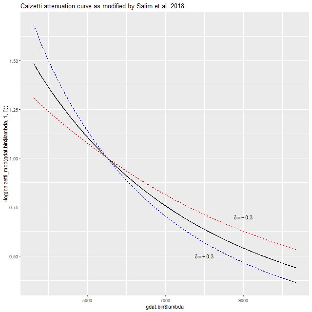
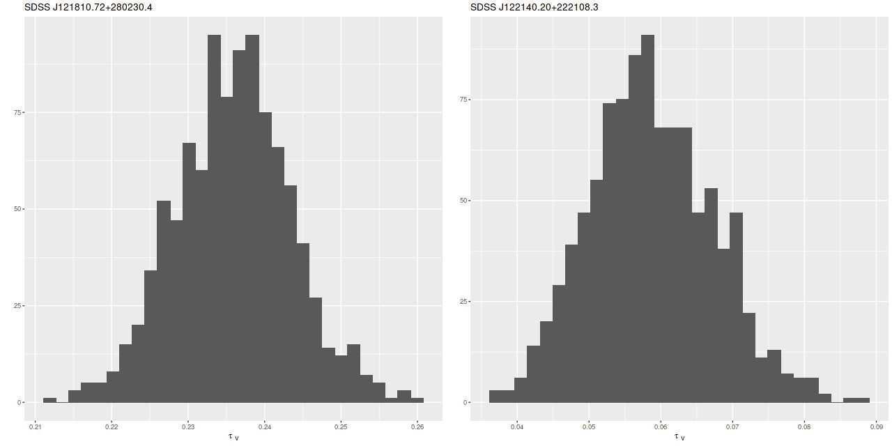
The functions block at the top of the code defines the modified Calzetti attenuation relation that I’ve been discussing in the last several posts. This adds a single parameter delta to the model that acts as a sort of slope difference from the standard curve. As I explained in the last couple posts I give it a tighter prior in the model block than seems physically justified.
There are two sets of parameters for the stellar contributions declared in lines 36-37 of the parameters block. Besides the simplex declaration for the individual SSP contributions there is an overall multiplicative scale parameter a. The way I (re)scale the data, which I’ll get to momentarily, this should be approximately unit valued. This is expressed in the prior in line 44 of the model block. Even though negative values of a would be unphysical I don’t explicitly constrain it since the data should guarantee that almost all posterior probability mass is on the positive side of the real line.
The current version of the code doesn’t have an explicit prior for the simplex valued SSP model contributions which means they have an implicit prior of a maximally dispersed Dirichlet distribution. This isn’t necessarily what I would choose based on domain knowledge and I plan to investigate further, but as I discussed in that post I linked it’s really hard to influence the modeled star formation history much through the choice of prior.
In the MILES SSP models one solar mass is distributed over a given IMF and then allowed to evolve according to one of a choice of stellar isochrones. According to the MILES website the flux units of the model spectra have the peculiar scaling
\((L_\lambda/L_\odot) M_\odot^{-1} \unicode{x00c5}^{-1}\)
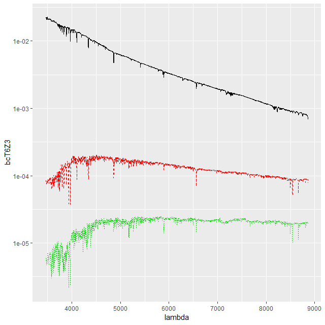
This convention, which is the same as and dates back to at least BC03, is convenient for stellar mass computations since the model coefficient values are proportional to the number of initially solar mass units of each SSP. Calculating quantities like total stellar masses or star formation rates is then a relatively trivial operation. Forward modeling (evolutionary synthesis) is also convenient since there’s a straightforward relationship between star formation histories and predictions for spectra. It may be less convenient for spectrum fitting however, especially using MCMC based methods. The plot below shows a small subset of the SSP library that I’m currently using. Not too surprisingly there’s a multiple order of magnitude range of absolute flux levels with the main source of variation being age. What might be less evident in this plot is that in the units SDSS uses coefficient values might be in the 10’s or hundreds of thousands, with multiple order of magnitude variations among SSP contributors. A simple rescaling of the library spectra to make at least some of the coefficients more nearly unit scaled will address the first problem, but won’t affect the multiple order of magnitude variations among coefficients.
One alternative that’s close to standard statistical practice is to rescale the individual inputs to have approximately the same scale and central value. A popular choice for SED fitting is to normalize to 1 at some fiducial wavelength, often (for UV-optical-NIR data) around V. For my latest model runs I tried renormalizing each SSP spectrum to have a mean value of 1 in a ±150Å window around 5500Å, which happens to be relatively lacking in strong absorption lines at all ages and metallicities.
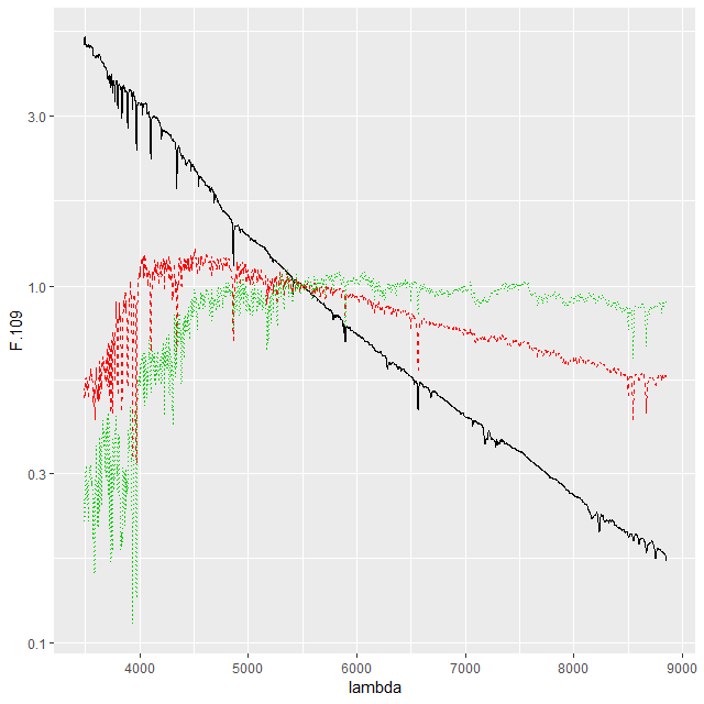
This normalization makes the SSP coefficients estimates of light fractions at V, which is intuitively appealing since we are after all fitting light. The effect on sampler performance is hard to predict, but as I said at the top of the post a combination of light weighted fitting with the stellar contribution vector declared as a simplex seems to have favorable performance both in terms of execution time and convergence diagnostics. That’s based on a very small set of model runs and no rigorous performance comparisons at all2among other issues I’ve run versions of these models on at least 4 separate PCs with different generations of Intel processors and both Windows and Linux OSs. This alone produces factor of 2 or more variations in execution time..
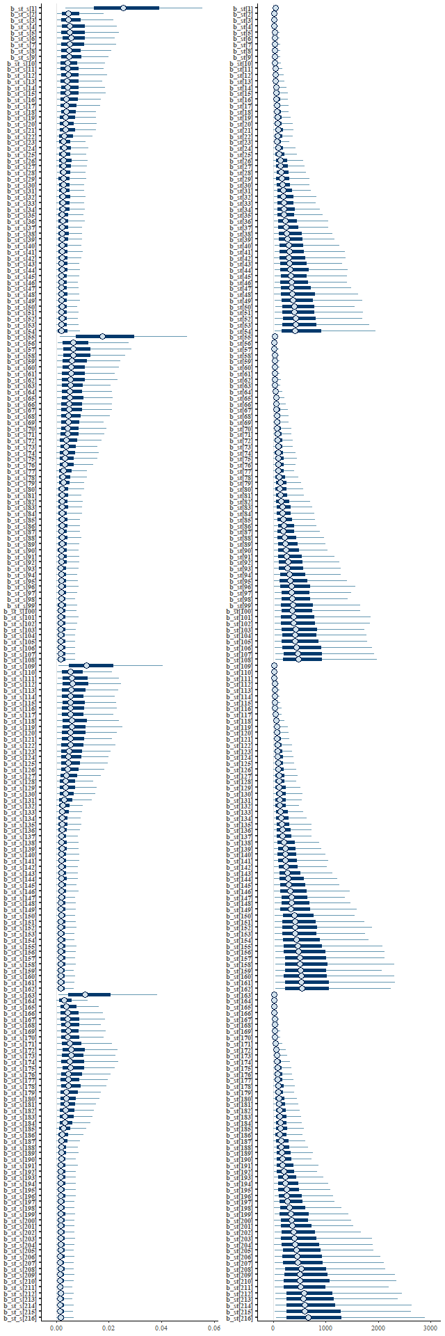
For a quick visual comparison here are coefficient values for a single model run on a spectrum from somewhere in the disk of the spiral galaxy that’s been the subject of the last few posts. These are “interval” plots of the marginal posterior distributions of the SSP model contributions, arranged by metallicity bin (of which there are 4) from lowest to highest and within each bin by age from lowest to highest. The left hand strip of plots are the actual coefficient values representing light fractions at V, while the right hand strip are values proportional to the mass contributions. The latter is what gets transformed into star formation histories and other related quantities. The largest fraction of the light is coming from the youngest populations, which is not untypical for a star forming region. Most of the mass is in older populations, which again is typical.
Another thing that’s very typical is that contributions come from all age and metallicity bins, with similar but not quite identical age trends within each metallicity bin. I find it a real stretch to believe this tells us anything about the real chemical evolution distribution trend with lookback time, but how to interpret this still needs investigation.