
Now that I have some data in a form suitable for further analysis my next step is to estimate radial velocity offsets. Part of the metadata is a system redshift z taken from the MaNGA observation catalog, which in turn is derived from the NSA catalog. Most redshifts are from the SDSS legacy survey, and usually but not always the spectroscopic target is close to the system nucleus, which is generally at the IFU center. What I actually measure then are redshift offsets from the cataloged system redshift, and I expect those most of the time to be small. The algorithm I developed uses a straightforward, not quite brute force template matching procedure that I believe, without having seen the code, is similar to that used in the SDSS spectro pipeline. This is a simpler task though because there’s no need to distinguish among stars, galaxies, and QSO’s and the range of redshifts to be probed is much smaller.
The templates I use are a set of 15 eigenspectra from a principal components analysis of ∼16,000 SDSS legacy survey galaxy spectra using an algorithm published by Tsalmantza and Hogg (2012). These are of some independent interest, but I will defer writing about them until a later post. The algorithm returns a single blended estimate for both stars and ionized gas. This differs from the MaNGA science team’s data analysis pipeline which produces separate estimates for stars and gas. From the small number of thumbnail size plots of velocity fields that have been published it’s evident that one or the other of these estimates is usually significantly noisier. Blended estimates should be cleaner provided ionized gas and stars are kinematically tightly coupled. This isn’t always true — in fact there is at least one published paper studying MaNGA galaxies with kinematically decoupled gas and stars (Jin et al. 2016). It also performs poorly if multiple velocity components are present, as in ongoing mergers, or if spectra are contaminated by foreground stars.
For completeness, and because the function is fairly small I reproduce the code here:
getdz <- function(gdat, lib, snrthresh=5, nlthresh=2000, dzlim=0.003, searchinterval=1e-4) {
  dims <- dim(gdat$flux)
  nr <- dims[1]
  nc <- dims[2]
  dz <- matrix(NA, nr, nc)
  dz.err <- matrix(NA, nr, nc)
  z <- gdat$meta$z
  lambda <- gdat$lambda
  fmla <- as.formula(paste("f ~", paste(names(lib)[-1], collapse="+")))
  fn <- function(x) {
    lambda.out <- lambda/(1+z+x)
    lib.out <- regrid(lambda.out, lib)
    lfit <- lm(fmla, data=lib.out, weights=iv)
    deviance(lfit)
  }
  fn_v <- Vectorize(fn)
  z_search <- seq(-dzlim, dzlim, by=searchinterval)

  for (i in 1:nr) {
    for (j in 1:nc) {
      if (is.na(gdat$snr[i,j]) || gdat$snr[i,j]<=snrthresh) next
        f <- gdat$flux[i, j, ]
        if (length(which(!is.na(f))) < nlthresh) next
          iv <- gdat$ivar[i, j, ]
          dev_grid <- fn_v(z_search)
          z0 <- z_search[which.min(dev_grid)]
          bestz <- Rsolnp::solnp(pars=z0, fun=fn,
                                 LB=z0-searchinterval, UB=z0+searchinterval,
                                 control=list(trace=0))
          dz[i,j] <- bestz$pars
          dz.err[i,j] <- sqrt(2./bestz$hessian)
    }
  }
  list(dz=dz, dz.err=dz.err)
}
I’ll review a few points about this function. The arguments gdat and lib are the IFU data described in the last post and a data frame with the rest frame template wavelengths and eigenspectra. I’ve found that sometimes large portions of spectra are masked by the DRP; often these are near the edge of the IFU and have very low signal to noise, so I set a minimum threshold for number of unmasked wavelength bins. The other arguments with default values just set reasonable limits for SNR, maximum redshift deltas, and grid size for preliminary search.
The function fn is the key section of code. Given the system redshift and a trial offset given in the function argument it calculates the galaxy restframe wavelengths, regrids the eigenspectra library to that vector of wavelengths, then fits it to the galaxy spectrum by weighted least squares and returns the deviance (weighted sum of squares). This function takes advantage of R’s rather peculiar scoping rules. When R encounters a name it checks the current environment for a value. If it finds one it uses it, otherwise it checks the parent environment, and if necessary the parent of the parent, etc. until it either finds the name or runs out of environments.
Just below the function definition I use the built in R function Vectorize, which takes a function that returns a single value and creates a new function that returns a vector. The brute force part of this code is a search over a uniformly spaced grid to isolate an interval containing the global minimum. This calls the vectorized version fn_v of fn, thus avoiding an explicit loop (which are generally best avoided in R). This also lets me write the grid search portion in two lines of code, which could have been condensed to one. Finally I use a general nonlinear optimization routine to refine the redshift offset estimate. I’ve found the function solnp in the independently developed Rsolnp package to be somewhat more robust than R’s built in options, but for this application it’s somewhat of an overkill. The return value from the function is a list of redshift offsets and uncertainties estimated from the local curvature. Here by the way is another R peculiarity. The value returned by a function is the last expression evaluated, which in this case is just the creation of a named list. Although there is a built in function return() nobody seems to quite know what it actually does and it’s rarely necessary to use it.
This function has considerable room for efficiency improvements. For one thing this task is embarrassingly parallel since each spaxel/fiber is evaluated independently, so this could easily be broken into chunks and fed to multiple cores when available. Also, the built in R function lm() for linear modeling does more than necessary and is somewhat slower than just doing the matrix algebra. So this function may change in the future.
Let’s take a look at a few examples. I modified the code to return the grid of deviance values for a single input spectrum. For this illustration I took the spectra from the eastern-most, central, and western-most fiber/pointing combinations from the stacked RSS data. The spectra are shown in the top row, with the run of deviance values with redshift offset in the bottom. Note there are many local minima in the deviance plots for the two corner spectra, which have very low S/N. This is probably due to accidental alignments of noise spikes with features in the eigenspectra rather than actual overlapping component populations. Somewhat surprisingly though the valleys in the vicinity of the global optima are even more steep sided than that for the central fiber, so the redshift offsets are quite well constrained. The presence of local optima is problematic for most nonlinear optimizers, which is why I use a brute force search to isolate global optima.
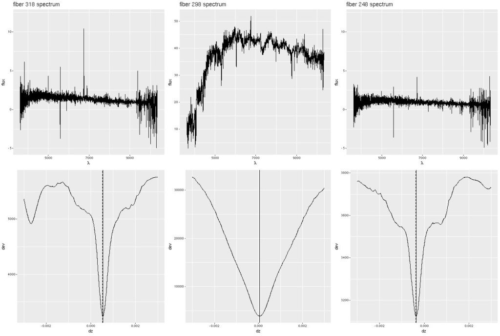 Deviance vs. delta z for 3 fiber/pointing combinations
Next are the full velocity fields, first from the stacked RSS data and below it from the data cube. I set a signal to noise threshold of 3 for these, which seems optimistic but is usually OK for extracting velocities. The symbols in the first graph aren’t quite to scale — the fiber positions actually overlap somewhat. In the second graph contour lines are separated by 25 km/sec.
Experts in data visualization generally frown on the use of rainbows, but I think they’re OK for this one specific application. In my shared code I define
rainbow <- c("blue", "cyan", "green", "yellow", "red") as the set of additive and subtractive primary colors from blue through red. In ggplot2 plots of continuous variables this gets expanded to a fairly perceptually uniform spectrum optimized for display on a monitor.
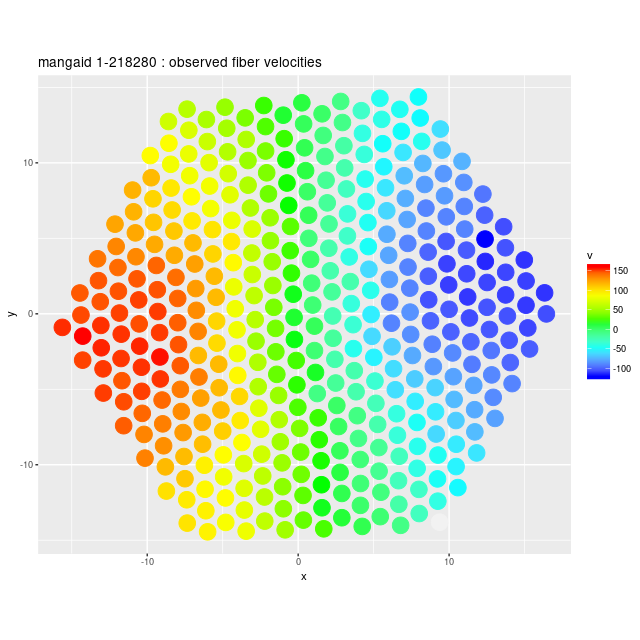 Example velocity field
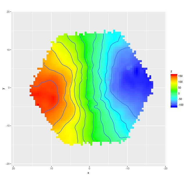 Example velocity field from data cube
I’m going to take a little closer look at the comparison between the RSS derived velocity field and the one from the cube. First I use the function interp from the package akima to interpolate the RSS data onto the same 74×74 grid as the data cube. The code to do that and display the results is:
> allok <- complete.cases(dv.stack)
> dv.interp <- akima::interp(x=gdat.stack$xpos[allok], y=gdat.stack$ypos[allok], z=dv.stack[allok], xo=-3600*gdat.cube$xpos, yo=3600.*gdat.cube$ypos, linear=FALSE)
> ggimage(dv.interp$z, dv.interp$x, dv.interp$y, col=rainbow, addContour = T, binwidth = 25, legend="dv km/sec")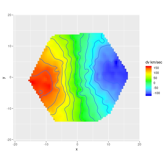
These look pretty similar. Taking the difference:
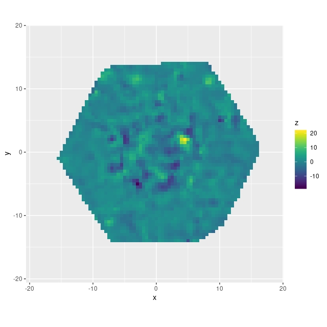
There’s some possible structure here — there’s an irregular ring of negative velocity differences punctuated with a small area of positive difference. It’s a little hard to relate these to features in the galaxy (and I’d like to develop better tools for this), but comparing to the SDSS supplied thumbnail with superposed IFU footprint the ring might correspond to the inner arms and perhaps where the bar meets the arms:

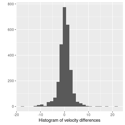
We’ll see later that arms and bars do measurably perturb velocities, and this suggests that different interpolation schemes might affect the fine details. But this is a higher order problem. Overall the velocity differences are symmetrically distributed around 0, with a standard deviation of just 2.7 km/sec and just slightly heavy tails:
Next up — doing something with velocity fields…