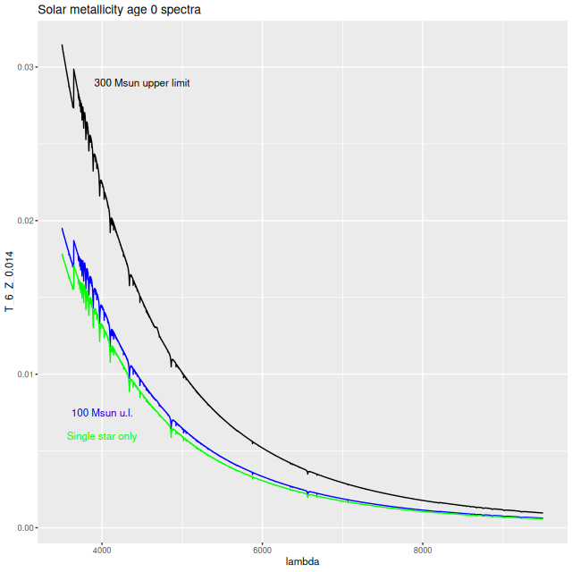
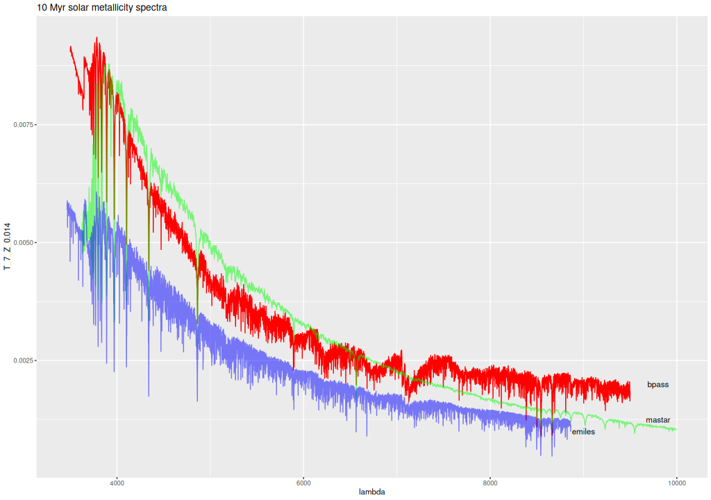
I’ve decided to take a break from real galaxy data and run some simulations of synthetic galaxy spectra. The main motivation was to help make an informed decision about which subset of the ProGeny based SSP libraries to use: the ones based on the MIST isochrones have ages uniformly logarithmically spaced at 0.05 dex intervals and 15 metallicity bins. Most of the latter are considerably sub-solar and aren’t likely to be major contributors to the light of nearby massive galaxies. For possibly metal poor dwarf galaxies it’s always possible to pick a metal poor subset — I have a subset of EMILES that I’ve used for that purpose for some time. More important to me is the choice of age bins. As I mentioned in the last post I did model runs with both 42 (0.1 dex age intervals) and 83 ages, with SSP models younger than log(T) = 6 and older than the currently accepted age of the universe excluded. Since execution time of a Stan model is roughly proportional to the number of parameters and these models are rather time consuming I’d like to know if the coarser age spacing has sufficient resolution. I will show below why it’s correct to exclude the very youngest populations.
Other reasons to do these kinds of exercises are to test the accuracy of retrieval of key quantities in idealized conditions where model assumptions are met by the inputs, to compare different model libraries, or to compare different modeling codes (something I don’t plan to do at present). Performing simulations is de rigueur in the SFH modeling industry and there are many examples in the literature, both as appendices and standalone papers — to name one the second of the two ProGeny papers I linked last time falls in this category. I’ve even done some limited simulations as far back as 2018, but the only case I wrote about was a very simple one.
This time I’ve decided to be more systematic and at least slightly more realistic. Since I remain interested in post-starburst galaxies I am creating simulations with two components: a base population that begins forming stars at the beginning of the universe, which I take to be a lookback time of \(10^{10.125}\) yr. = \(13.36\) Gyr. The second component is a “burst” population that commences star formation at a lookback time of \(\mathsf{t}_b\) with a relative strength of \(\mathsf{f}_b\). The base population has solar metallicity (Z = 0.02) while the burst is slightly subsolar (log(Z/Z☉) = -0.25). This obviously isn’t meant to represent a realistic model for chemical evolution — the purpose again is to test the ability to recover the input stellar metallicities in idealized circumstances. In keeping with my usual attitude of treating this as an afterthought I haven’t gotten around to exploring this issue yet.
Both the base and burst populations have time varying star formation rates proportional to Gamma probability distributions. The Gamma distribution is a two parameter family of univariate functions that can have a fairly wide variety of shapes, all of which have a single mode at \(t \ge 0\) followed by a monotonic decline asymptotically approaching 0. See the table below for the most salient properties. I don’t know of any real astrophysical justification1Abramson et al. (2016) argued for a log-normal form for the evolution of the cosmic SFR density and suggested that this describes the evolution of individual galaxies as well. More recently Katsianis, Yang, and Zheng (2021) argued for a gamma distribution fit to the evolution of the CSFRD and again claimed with some physical motivation that this form holds for individual galaxies. I was unaware of the latter work when I started this exercise. for this choice but it’s notable that it includes two of the most popular parametric forms for modeling star formation histories: exponentially declining (\(\alpha = 1\)), and what’s generally called the “delayed-\(\tau\)” model (\(\alpha =2\)) in the literature. Note that using a probability distribution has nothing to do with probability per se, but a probability density has two useful properties: it’s non-negative on its support and has a finite integral (equal to one when properly normalized).
| Property | Value |
| Parameters | shape \(\alpha \ge 0\) scale \(\theta > 0\) |
| Density function | \(f(t) = \frac{1}{\Gamma(\alpha)\theta^\alpha} t^{(\alpha-1)}\mathsf{e}^{-t/\theta}~~t \ge 0\) |
| Mean | \(\alpha\theta\) |
| Mode | \((\alpha -1)\theta~~\alpha\ge1\) \(0~~~~\alpha \le 1\) |
| Variance | \(\alpha \theta^2\) |
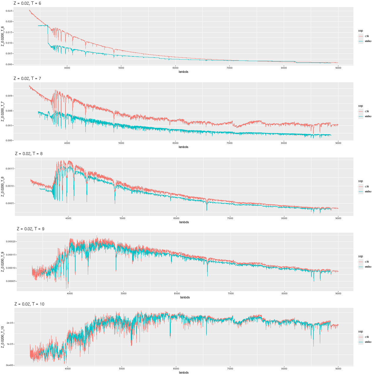
Given shape and scale parameters the mass in each time bin is proportional to the difference in the cumulative gamma distribution at the beginning and end of each interval. The star formation history for each component is just the mass formed in all age bins, with the burst component multiplied by the burst strength. These are scaled to sum to 1, and the spectra are straightforwardly calculated as matrix products of the input SSP model fluxes with the mass histories. The “flux” values are multiplied by 105 for the sole purpose of making them approximately unit scaled. This has the effect of making the total mass born in the simulated “galaxy” equal to 105 M☉. The fluxes are interpolated to the same logarithmic wavelength grid used by SDSS, convolved with a gaussian to simulate stellar velocity dispersion, then truncated to the wavelength range (3621 Å, 9000 Å). The velocity dispersion is a settable parameter, but so far I have only used 140 km/sec. The base and burst spectra, which were calculated separately for visualization purposes are added, then multiplied by Calzetti attenuation with a user selected optical depth, then finally perturbed with Gaussian random noise. The flux variances are Poisson-like, that is they are proportional to the “counts” in each wavelength bin and scaled to a target average signal to noise. Again this is a settable parameter, but so far I have used a target SNR of 40, which is fairly typical for a fiber spectrum near the center of the IFU of a bright MaNGA galaxy. So far at least I do not add emission lines, but they are allowed in the models.
The subsequent modeling workflow is essentially the same as I use with real data, with some very minor tweaks reflecting the fact that the flux values are arbitrarily scaled. The Stan code is exactly the same as my current working version. Model runs use the same number of warmup and sampling iterations as my real data runs (250 and 750 respectively with 4 independent chains). Post processing is also essentially the same. I extract the posterior predictive fits to the spectra, the model star formation histories, the optical depth of attenuation and the reddening curve slope parameter. I compute the present day stellar mass, the 100 Myr averaged star formation rates, and specific SFR. The stellar mass and SFR are arbitrarily scaled but would scale by the same factor if these were real data from a distant galaxy, so the SSFR would be the same.I also track a few observables: the 4000 Å break index Dn(4000) and HδA.
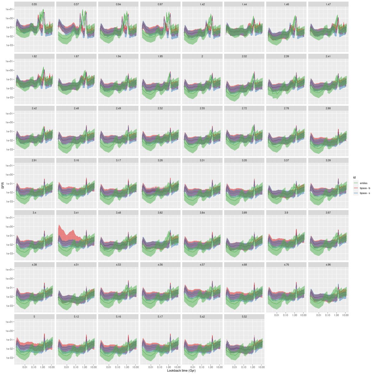
This time I am exploring a wider range of star formation histories than my previous effort, which only examined a case or two with instantaneous bursts. With seven parameters (plus two more that I’ve held constant so far) it isn’t really practical to do a comprehensive grid of models, so for the most part I have randomly selected parameter values in the ranges shown below. At the time of writing I’ve run a few more than a hundred models. Most of these use the “small” version of the ProGeny C3K base SSP models as the test library, with a few using the input library as the test. I’ve also done a few with the “large” version (see the previous post for details of the ingredients). I plan to do some simulations with the other model libraries I’ve used, especially EMILES, but that’s somewhat of a different project. For now I’m examining the accuracy of outputs for the idealized case where the inputs satisfy the assumptions of the model.
| \( \alpha_0 \in [1, 2] \) |
| \(\theta_0 \in [2, 6] \) |
| \(\mathsf{t}_b \in [0.5, 2]\) |
| \(\mathsf{f}_b \in [0.1, 0.75]\) |
| \( \alpha_b \in [1, 2] \) |
| \( \theta_b \in [0.01, 0.25] \) |
| \( \tau_V \in [0.0, 0.5] \) |
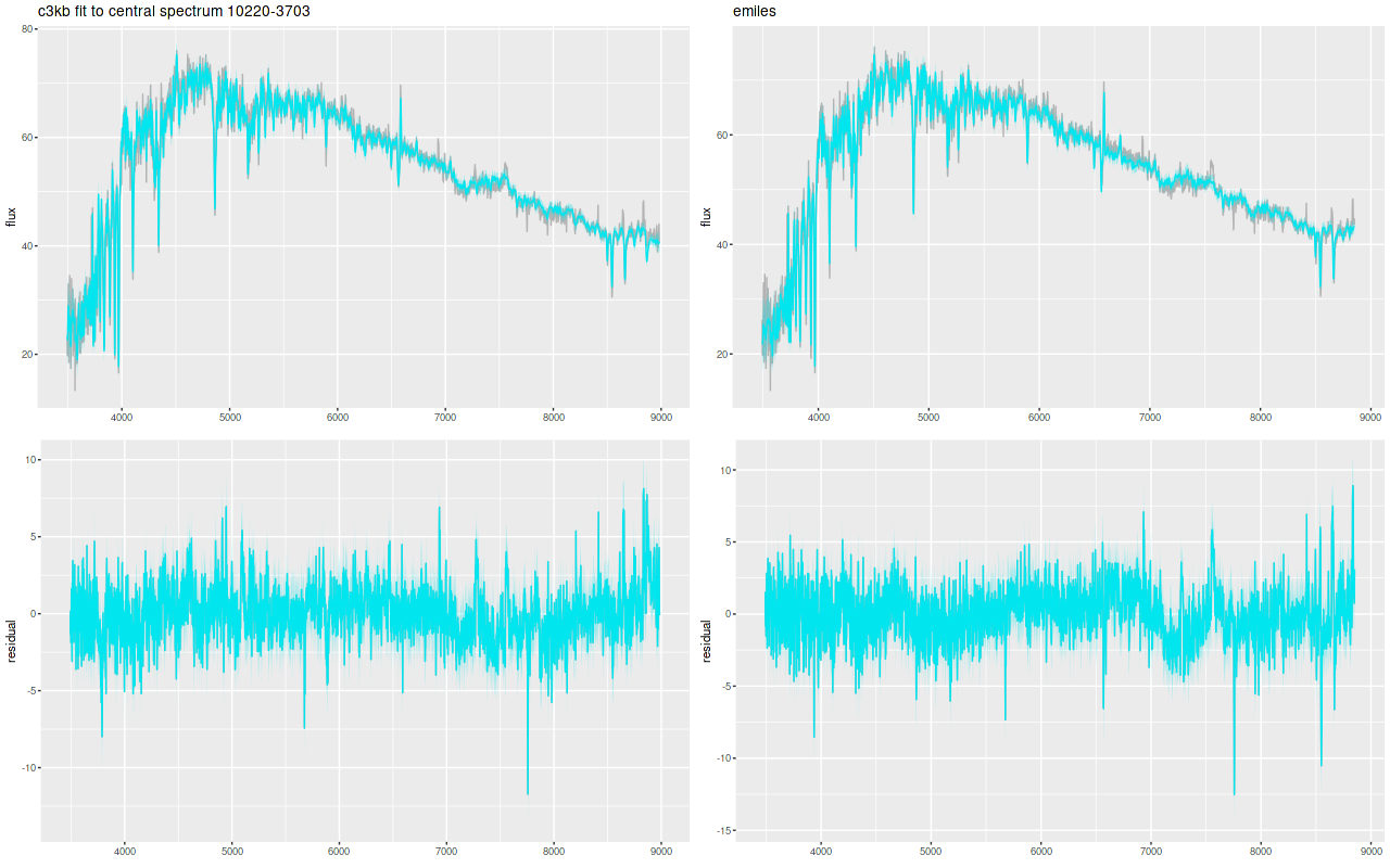
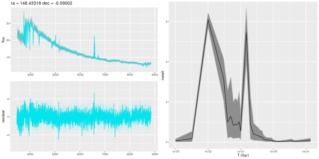
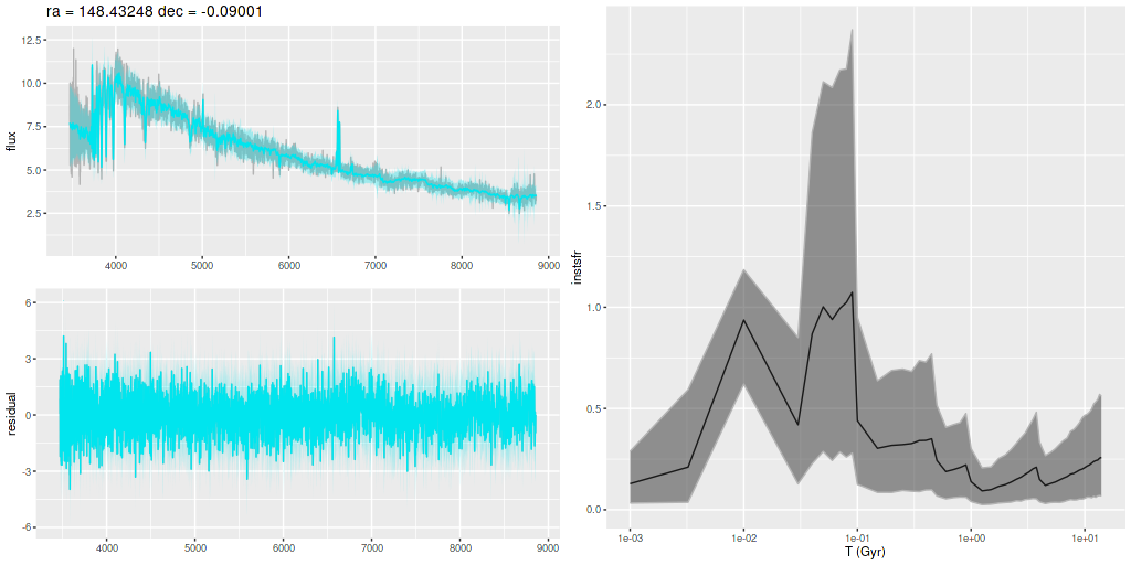
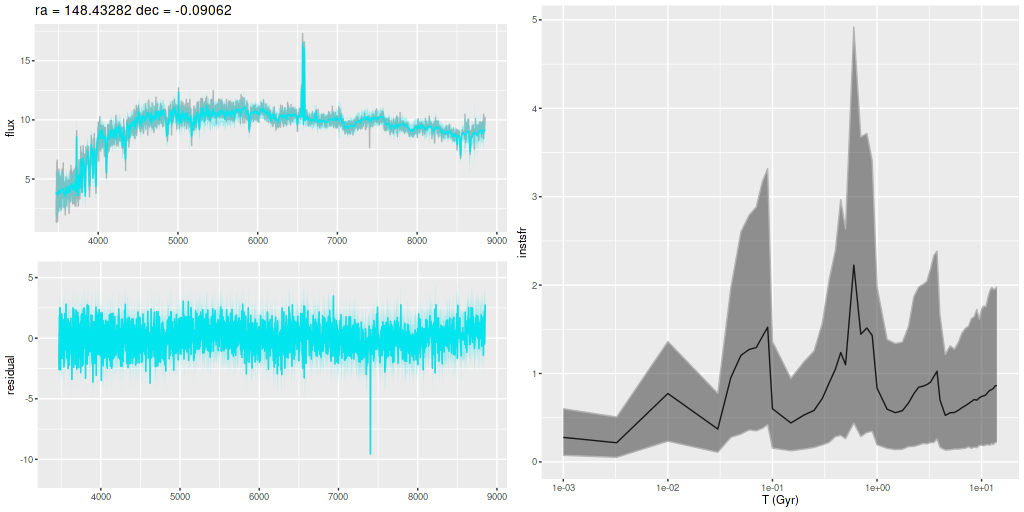
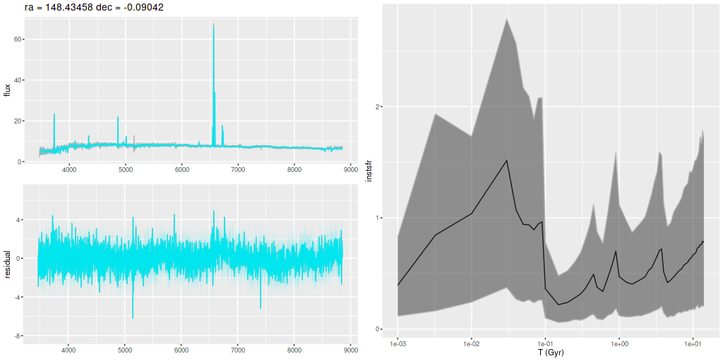
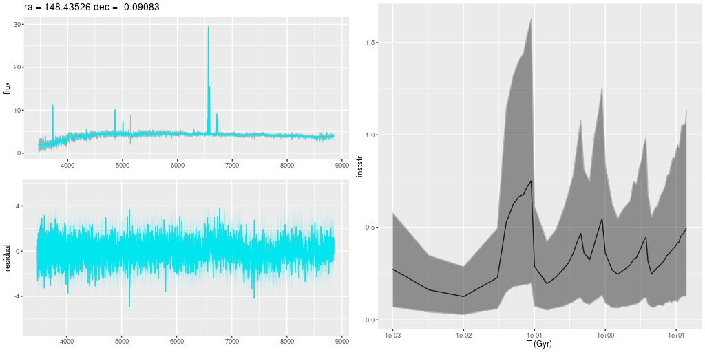
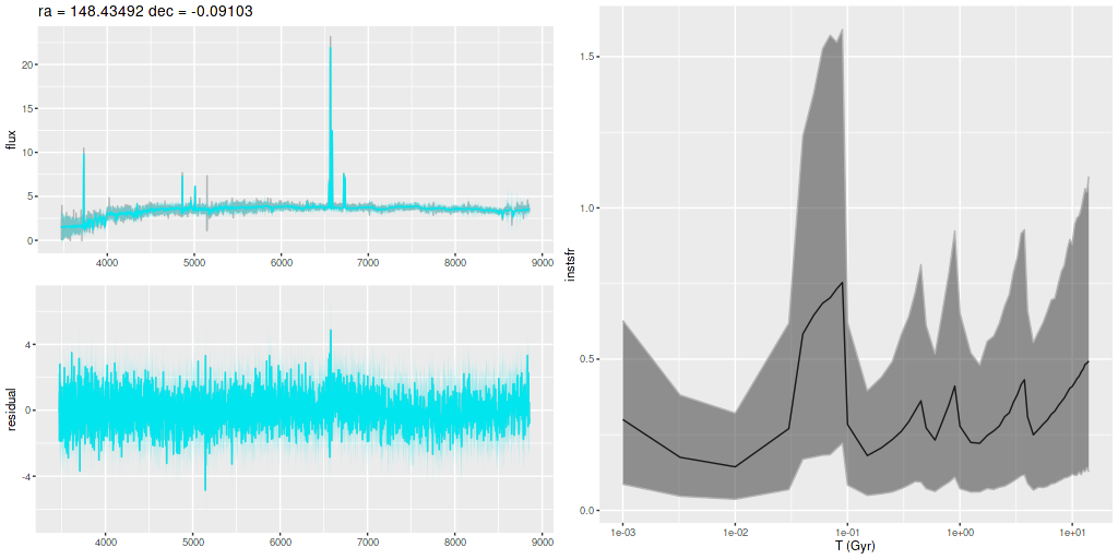
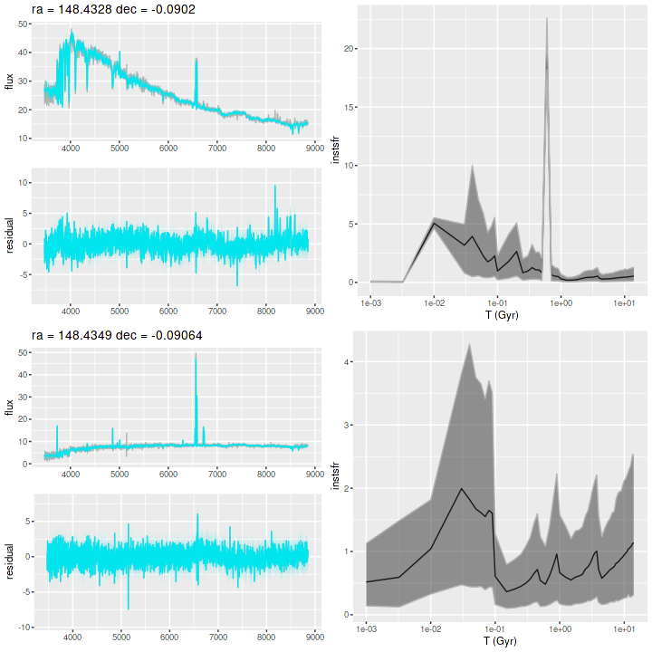
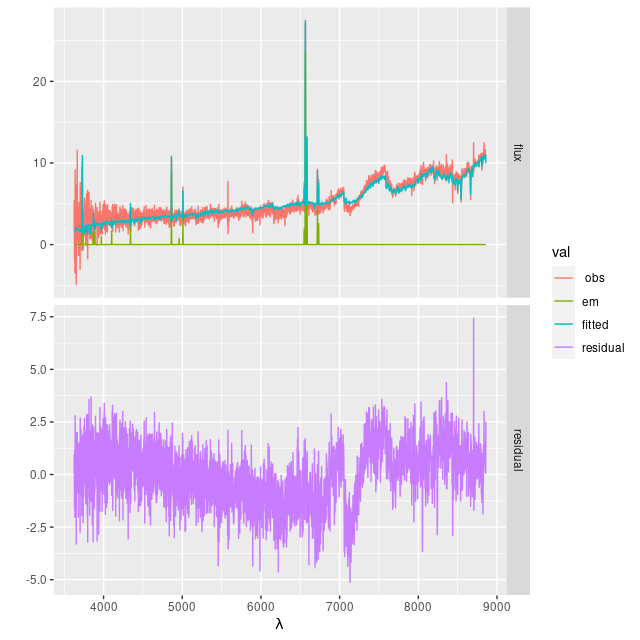
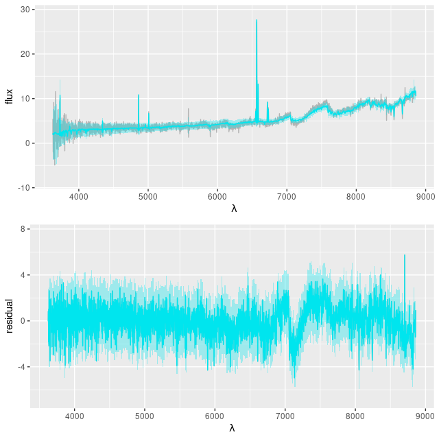
Here is a cherry-picked example of a fairly strong and recent burst, using the small C3K based library as the test. First is the “observed” spectrum and the replicated values from the posterior (top pane), and the posterior residuals (bottom pane). The residuals look very much like — and pass standard statistical tests for — Gaussian white noise. This is rather different than I usually see with real data, of which a number of examples can be found by scrolling down through previous posts, where there are often large regions of spectra that are systematically misfit. This reflects the fact that all model assumptions are met by the data by construction, so fitting the data is expected.

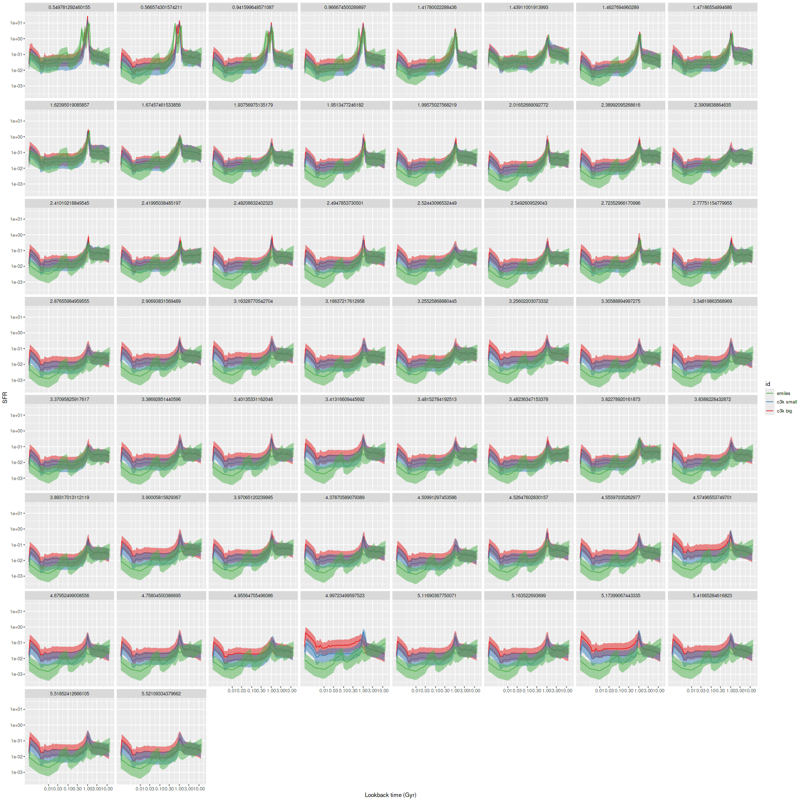
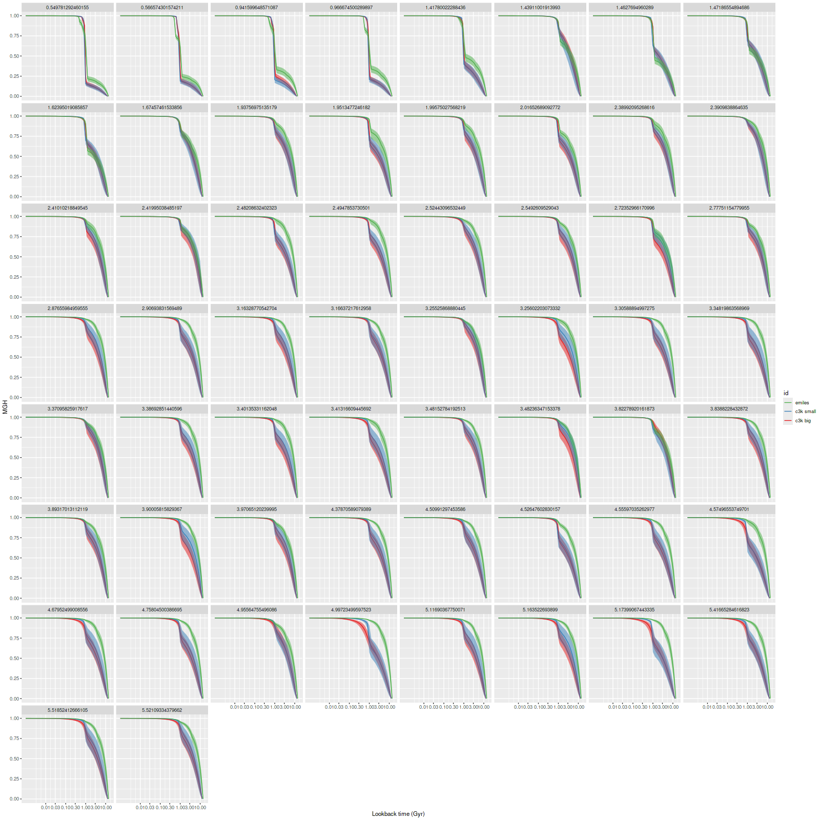
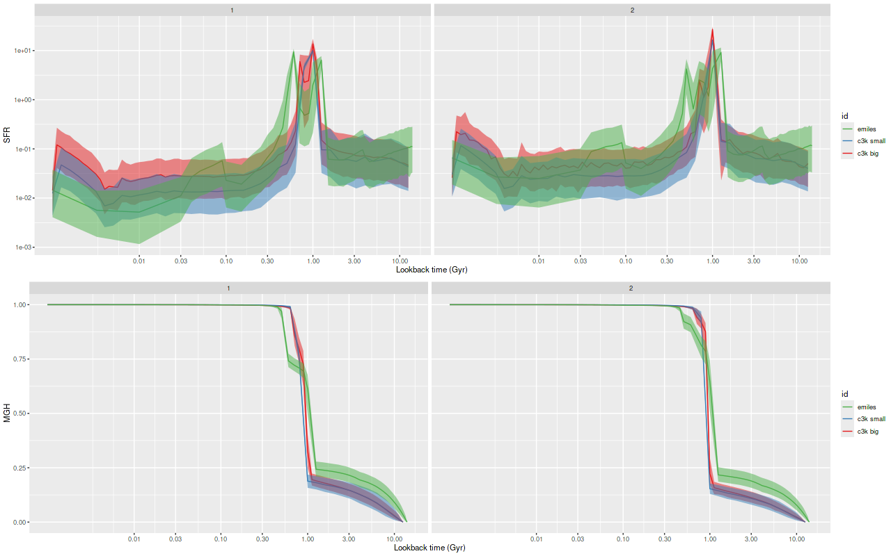
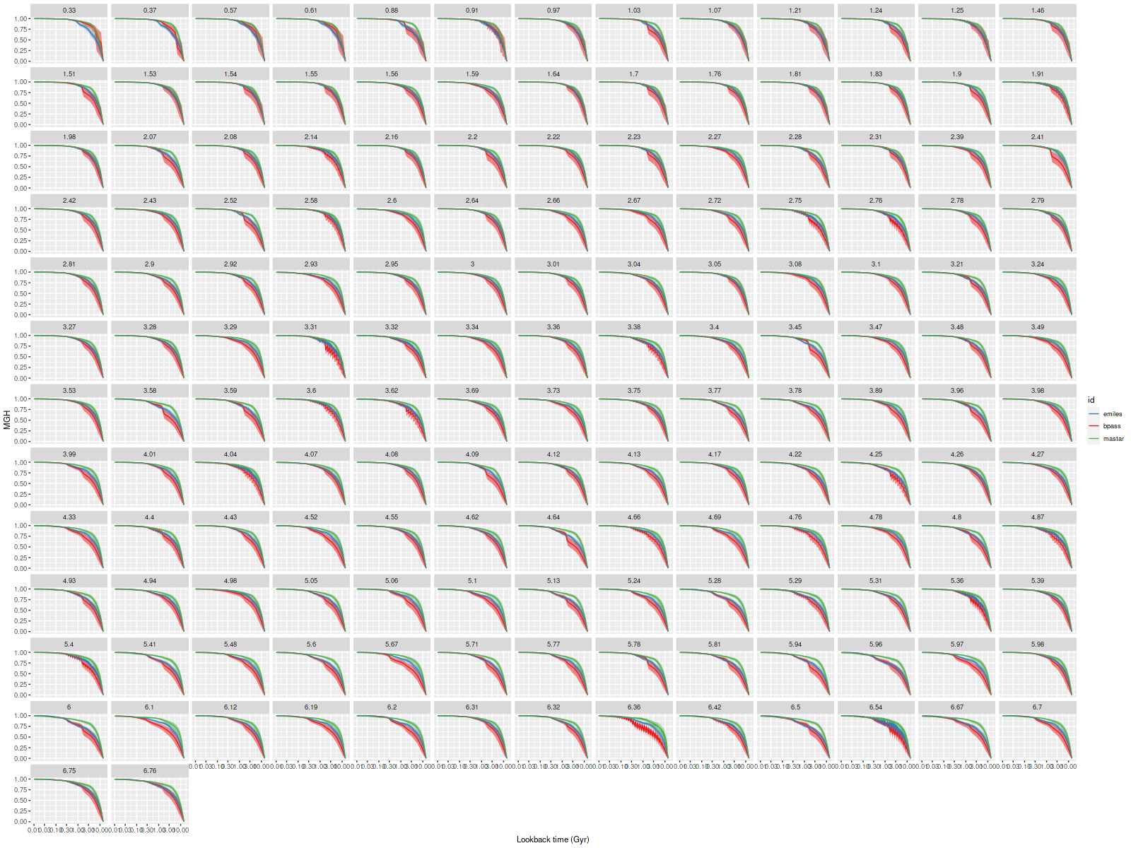
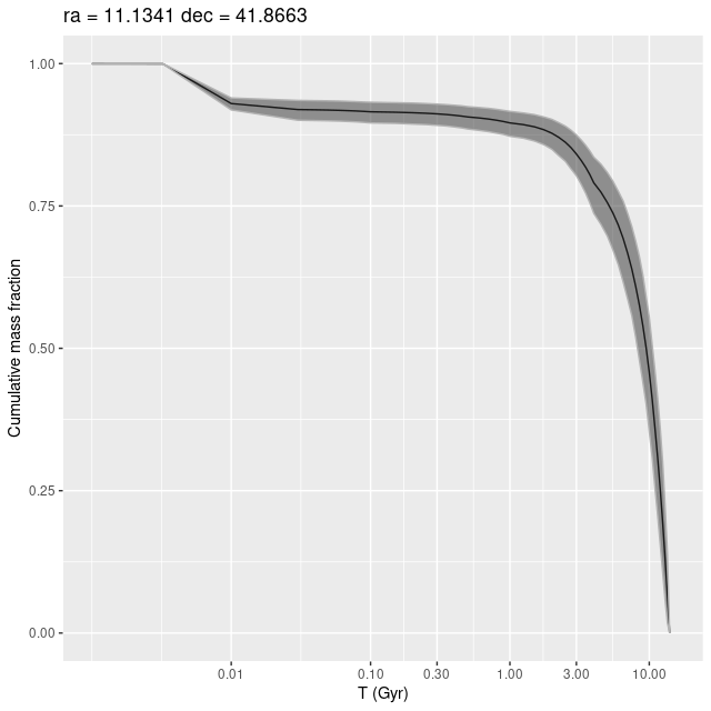
The model star formation history from the same simulated data contains some surprises, and these turn out to be fairly generic features of most model runs. This is a bit of a new graphical display for me. I’ve put the star formation rate history above the mass growth history with the same age scale for each so I can get different views of the same sequence of events. The input model parameters are on a line in between. The blue lines are the input star (mass) formation history. The red line in the second plot is from the preliminary maximum likelihood fit. The black lines and grey ribbons are the marginal means and 95% confidence intervals. Reading from right to left there are several points to note:
- The details of the pre-burst SFH are largely lost, although the total mass formed in the model is roughly the same.
- The ramp up to the peak of the burst begins sooner and is more gradual than the input. Note that both the input SFR and mass growth are well outside the model confidence intervals in the ramp up period.
- Most significantly in my mind at least, the peak of the burst is much later (more recent) in the model than the input. This turned out to be a fairly generic feature of these models.
- In this run the post-peak decay is rather steeper on average than the input. In model runs with a rapid input decay the model will usually have a more gradual one.
- The input and model SFR eventually converge and the late time model SFH agrees very well with the input, except
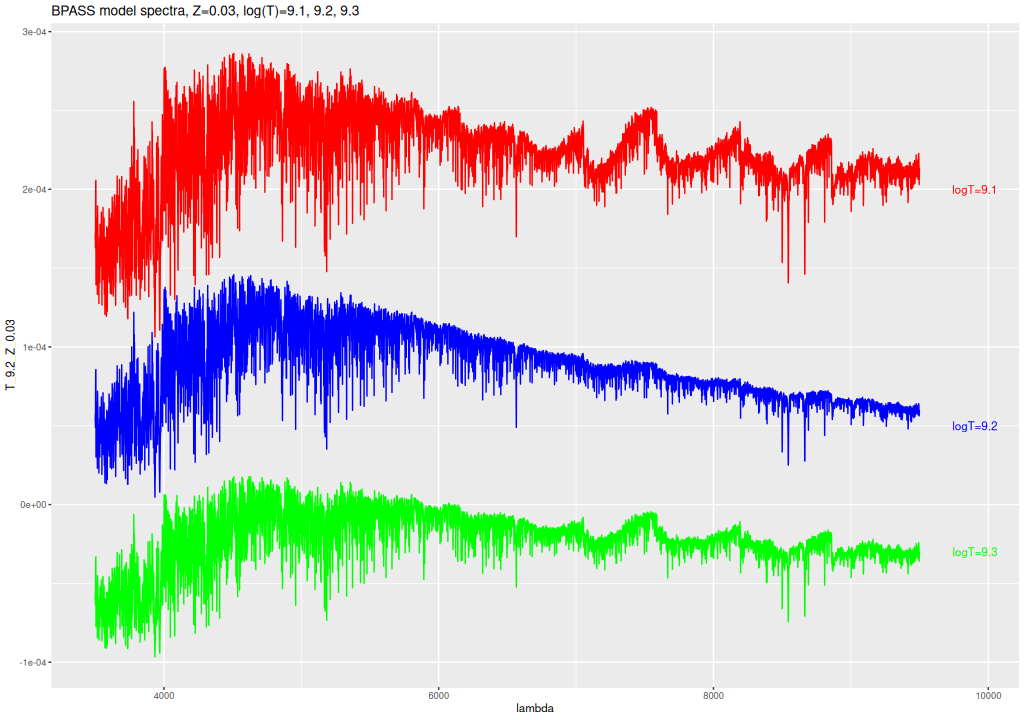
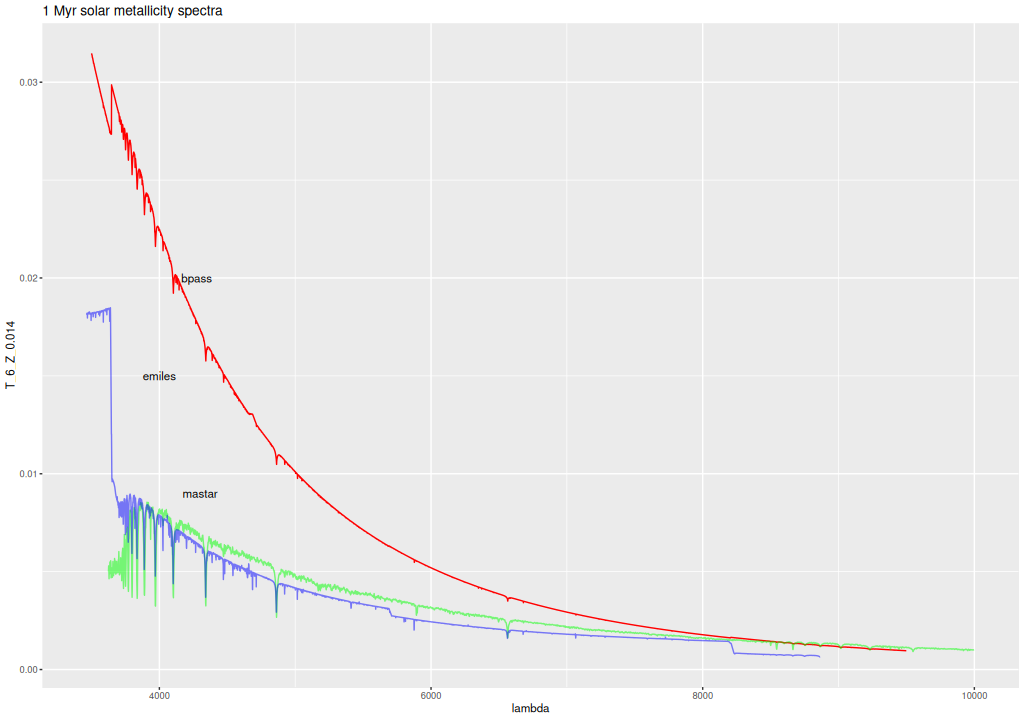
- There’s an odd upturn in SFR at the very youngest ages (< 3 Myr). This happens to varying degrees in every simulation model run and in all the real data I’ve looked at. It turns out there’s a simple explanation for this. There is virtually no spectroscopic evolution in the relevant wavelength range in the first few Myr of a coeval population’s life. Since the spectra are indistinguishable there is no way to constrain the individual contributions without a more informative prior, and the models are correctly estimating the same marginal distributions for the youngest few populations. Since the time intervals get shorter with decreasing age this produces an apparent upturn in SFR.


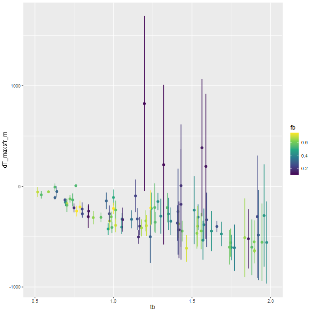
There are two surprises in the simulations I’ve run so far. First is that, like the example above, the time of peak star formation in the model burst tends to be biased downwards (more recent) from the input. The bias gets larger in magnitude with increasing lookback time to burst onset and can be as large as several hundred Myr as seen below. The few outliers here were weak bursts with very large variations in the time of maximum SFR.
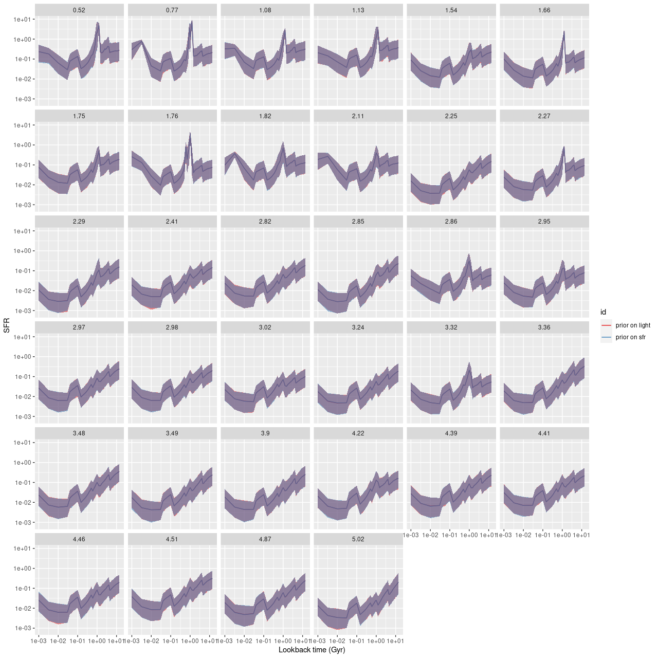
The other surprise is that the 95% confidence bands of the model star formation histories, whether viewed as SFR or mass growth histories, fail to cover the inputs for at least some epochs around the time of the burst. In other words the models are saying that the actual input star formation histories are highly unlikely. Why is this?
It’s not, I think, because of any convergence failure. Stan is quite aggressive at flagging potential issues and there were virtually none in any of the model runs. I also don’t think it’s because the model runs were too short. I’ve occasionally gathered much larger samples with longer warmup times as well and except for exploring the tails of the distributions a little more thoroughly there is little change in marginal 95% confidence intervals.
Most of the model runs were done with the reduced size SSP library with just half of the available age bins (0.1 dex intervals). This doesn’t seem to have reduced the real effective age resolution, but in the small number of runs I did with the full set of ages the marginal contributions have larger confidence intervals, so this could increase the coverage.
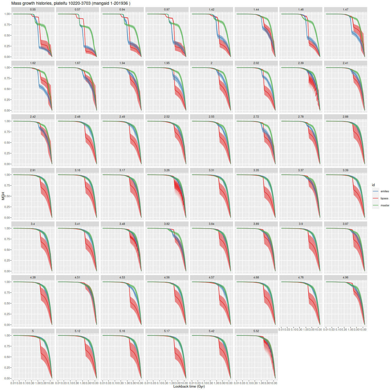
I suspect though that the prior on the star formation history is having a larger effect than I would have suspected. The main clues here are the maximum likelihood fits. which often produce mass growth histories (the red lines in the plot above and the ones below the fold below) that are rather close to the input MGH, also falling outside the 95% model confidence bands for at least some epochs. In my current workflow the slightly perturbed maximum likelihood solution is used to initialize the Stan model. In most of the model runs the samples quickly move away from the initial values. While the fits to the data are good in all model runs the summed log-likelihood of the sample spectra is always less than the maximum likelihood solution, in the sample shown below by about 7%.

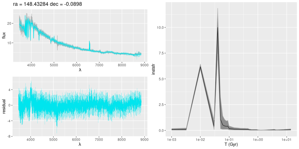
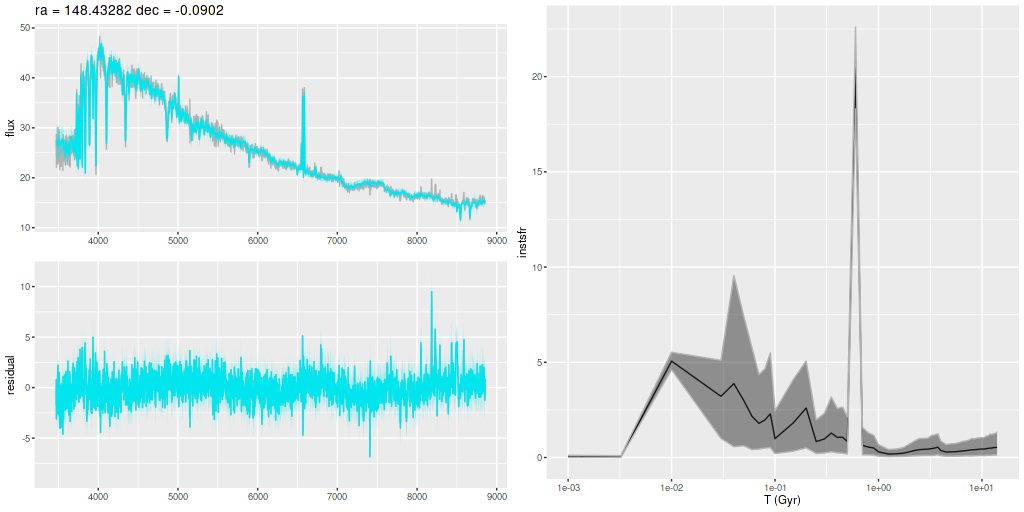
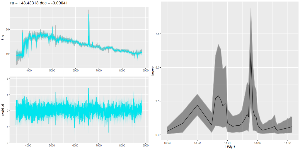
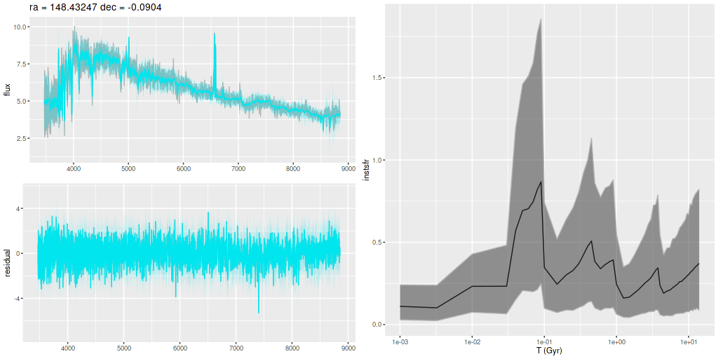
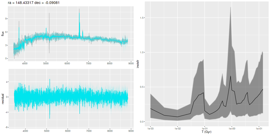
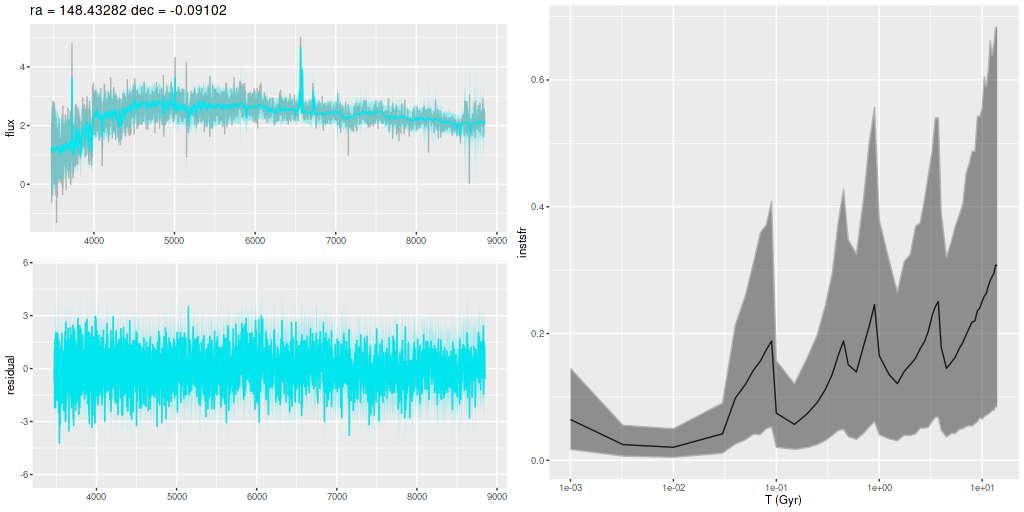
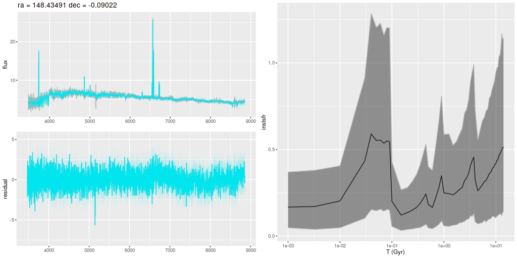
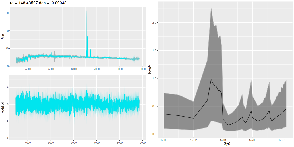
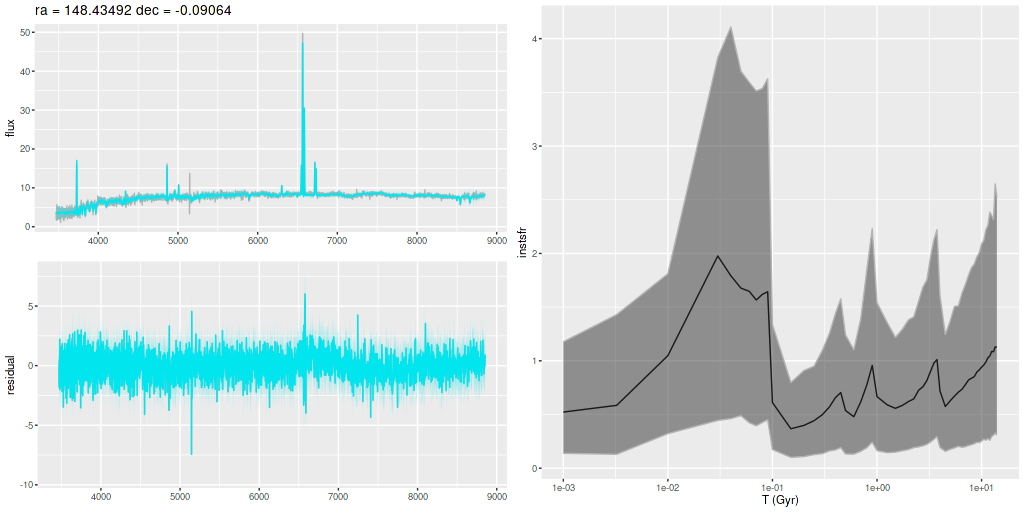
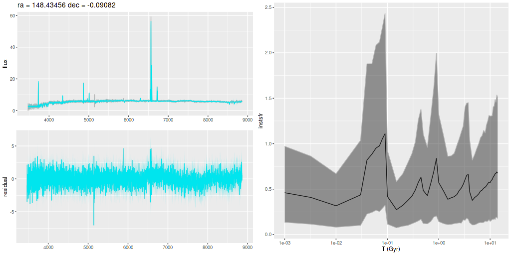
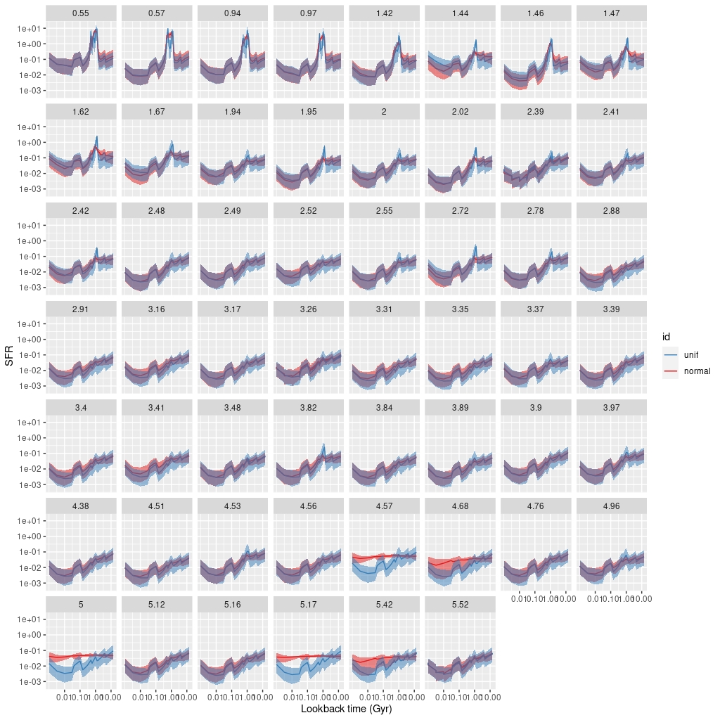
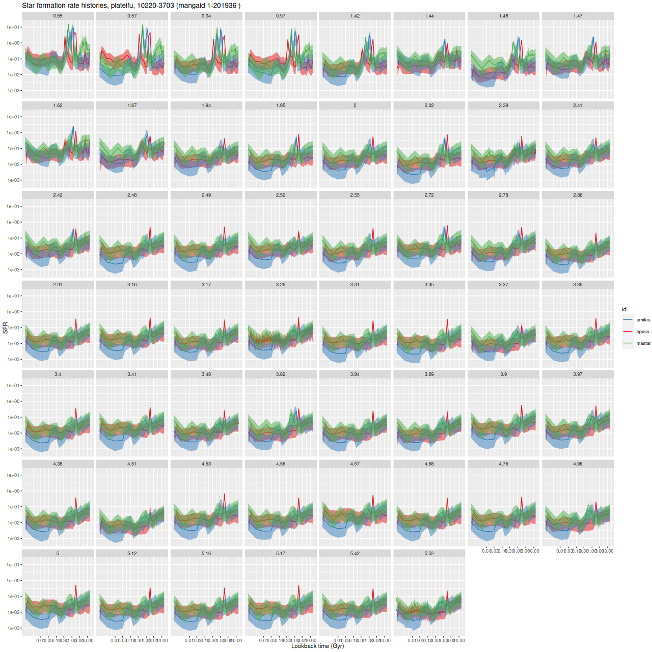
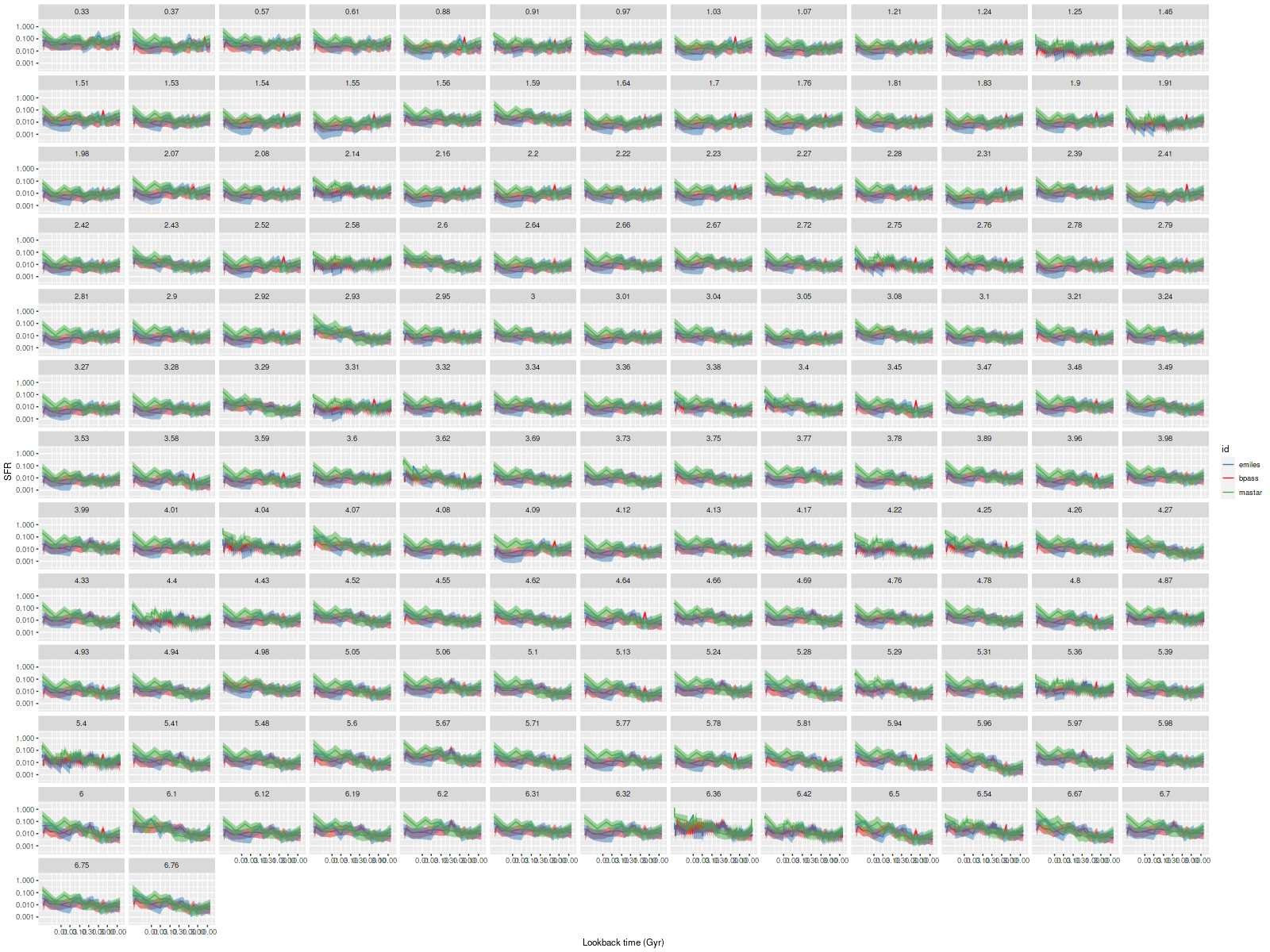
Below the fold I’ve posted some more cherry picked examples of model star formation histories. A few general comments about them:
- The late time star formation rate is generally well captured by the models.
- The ancient (pre burst) star formation history is sometimes captured well with weak bursts. Particulary noteworthy is the second example below, which has a recent and weak burst with a gradual ramp up and decay. The entire star formation history is modeled accurately. In the literature there are sometimes references to “outshining” or a “dazzle” effect in (post)-starburst galaxies. This seems to be a real thing.
- Early time bursts aren’t necessarily recognizable as such. In some cases the model just shows an extended period of star formation followed by more or less gradual quenching. I believe this is consistent with some claims in the literature, but I don’t care to look for the relevant papers right now.
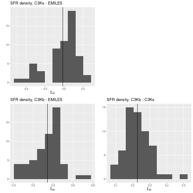
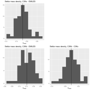
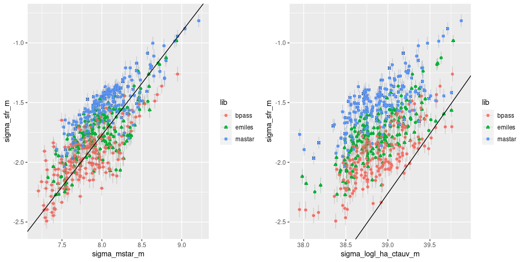
I’ll conclude with a look at results for all simulation runs (so far) for some of the summary quantities I track. First, the present day stellar mass is on average unbiased but in individual runs there are errors as large as ±0.1 dex. The typical posterior uncertainties are only ~0.01 dex, so the models are consistently too optimistic. I’ve noted this in real data, which shows similar nominal uncertainties with moderately high S/N data.
Not shown here but I did notice a weak dependence on the input burst onset time or time of maximum SFR in the sense that recent bursts tend to underestimate the stellar mass. This is another possible manifestation of the “outshining” effect.

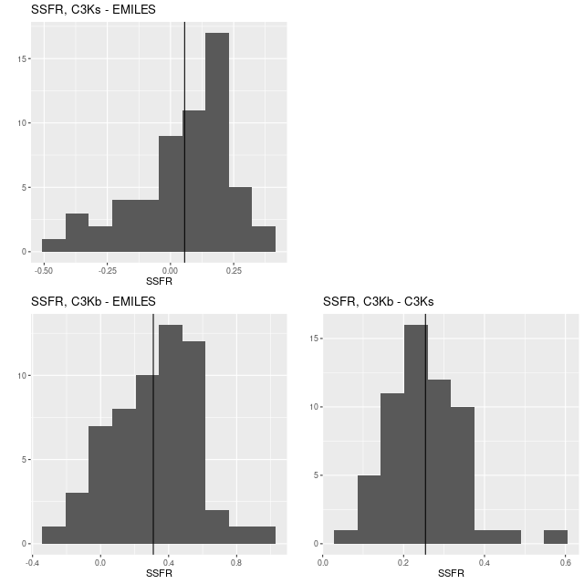
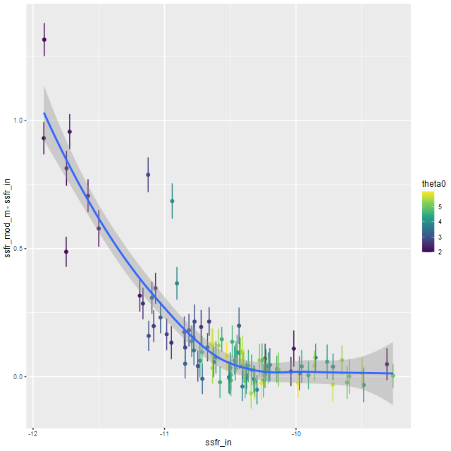
The most dramatic bias is a tendency to overestimate the specific star formation rate when the input SSFR is low. This is also something I’ve seen in real data: as I’ve noted a time or two even the reddest and deadest of ellipticals seem to have a floor of about -11.5 for the estimated SSFR.
One thing I didn’t think about until finishing this analysis is that the contribution estimates tend to be skewed to the right when they’re near 0, so the median might be a better estimate of central tendency than the mean. That might make a (probably) small difference. I will look into this.
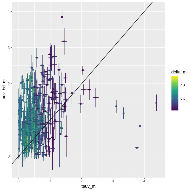
Finally, there’s a nearly linear relation between the error in the posterior estimate of the optical depth of attenuation and the input. Note also the stratification of the reddening slope parameter δ: at relatively high input optical depths the largest departures have the reddest attenuation curves. I think this behavior is directly related to the prior. Since I don’t think the attenuation is very well constrained by the data I use fairly informative priors on both the optical depth and slope parameter; both priors are truncated normals with a lower bound of 0 for τV and a range of (-0.5,1.2) for δ. This is an easy thing to test simply by changing the priors for these parameters.

I am not quite finished with these simulations. I want to expand the range of input parameters a little bit, and I need to look a little more carefully at subsets of the ProGeny SSP models. The main result so far is that my hopes of timing key events in post-starburst galaxies’ histories were probably too optimistic.
Continue reading “Back to simulating star formation histories”