sfh modeling – Extragalactic

2026-01-282026-01-30

NGC 2623 – part 3 – Stellar populations and star formation histories

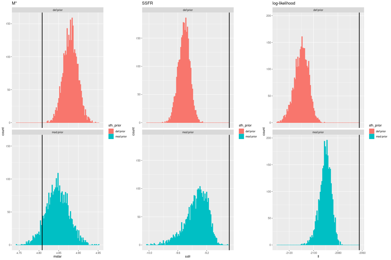
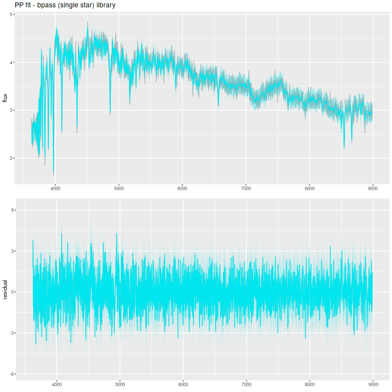
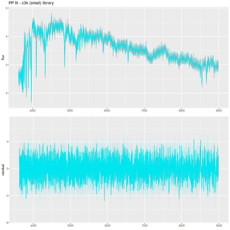
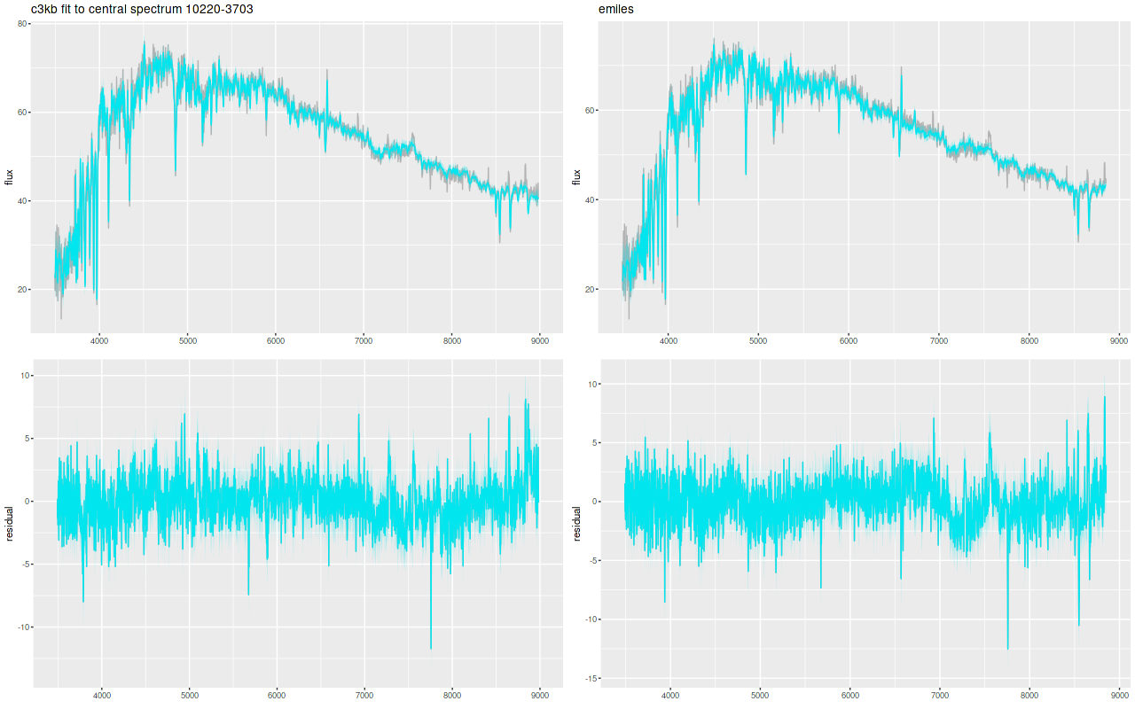
I am now, finally, going to turn to the properties of the stellar populations within the IFU footprint and detailed star formation history models. As a reminder these are based on my longstanding Stan language based code for nonparametric SFH modeling using what I refer to as the “medium” ProGeny based SSP model library as stellar inputs.

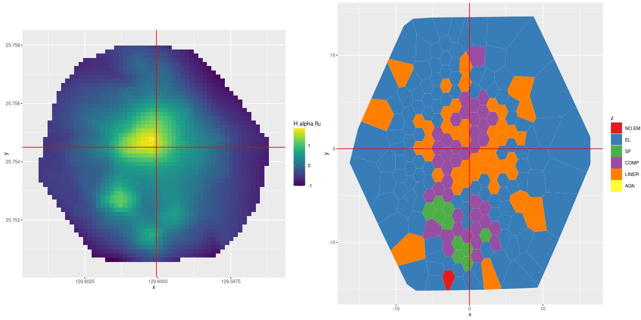
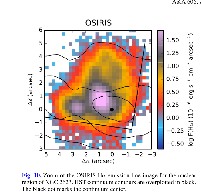
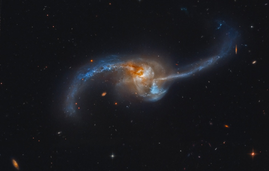
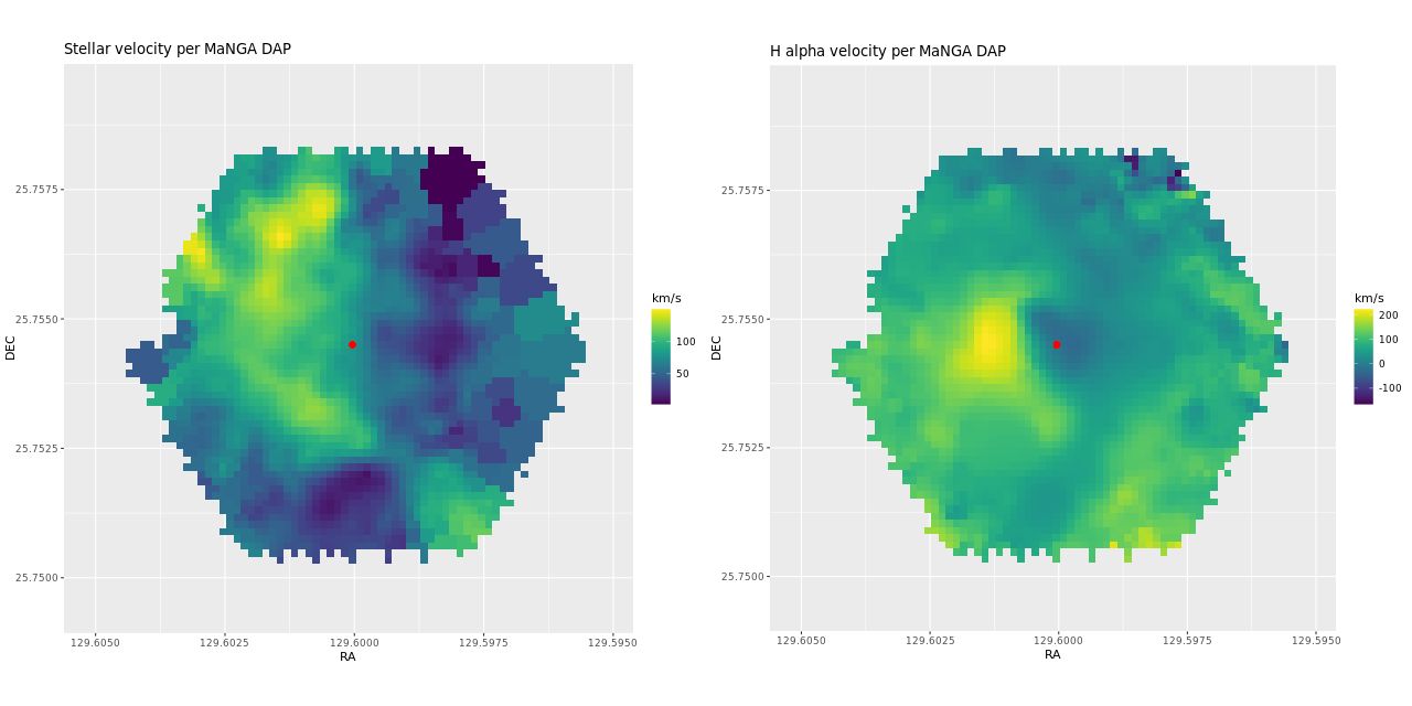
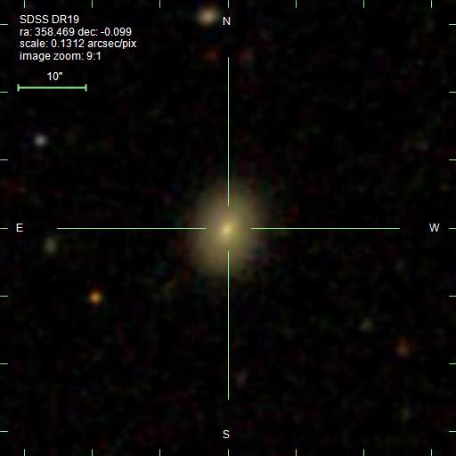
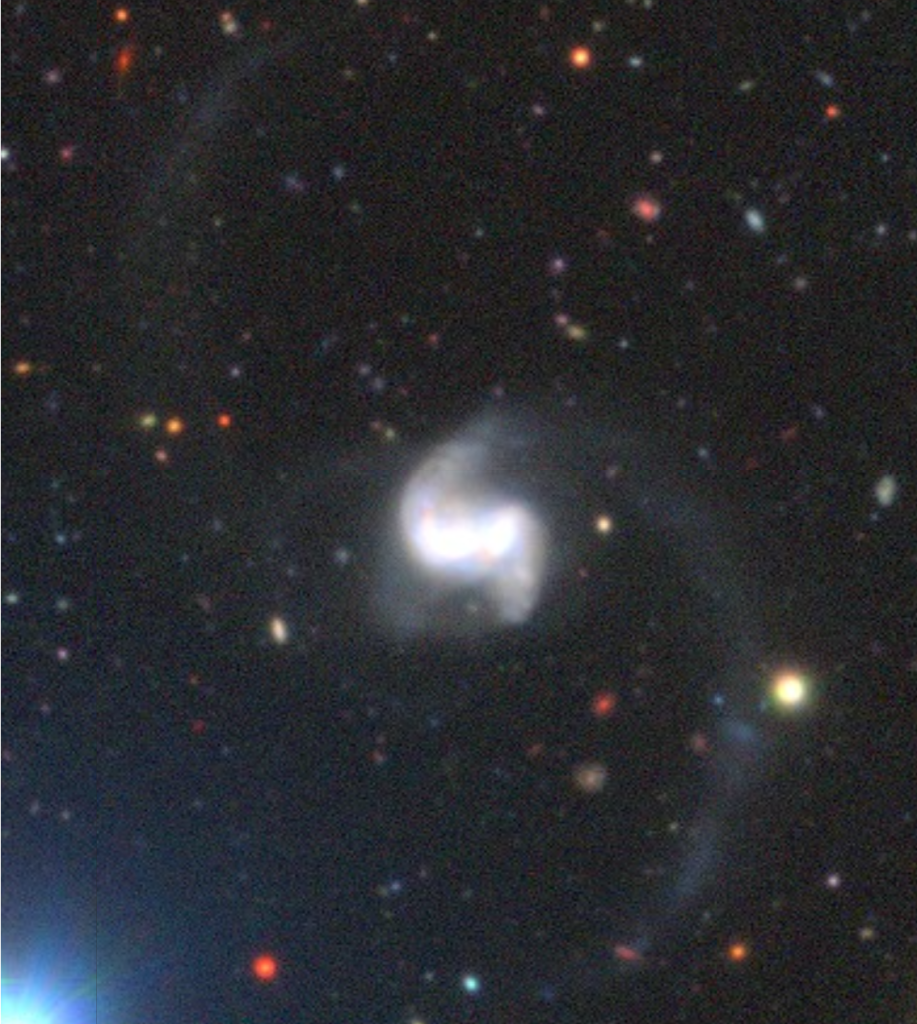
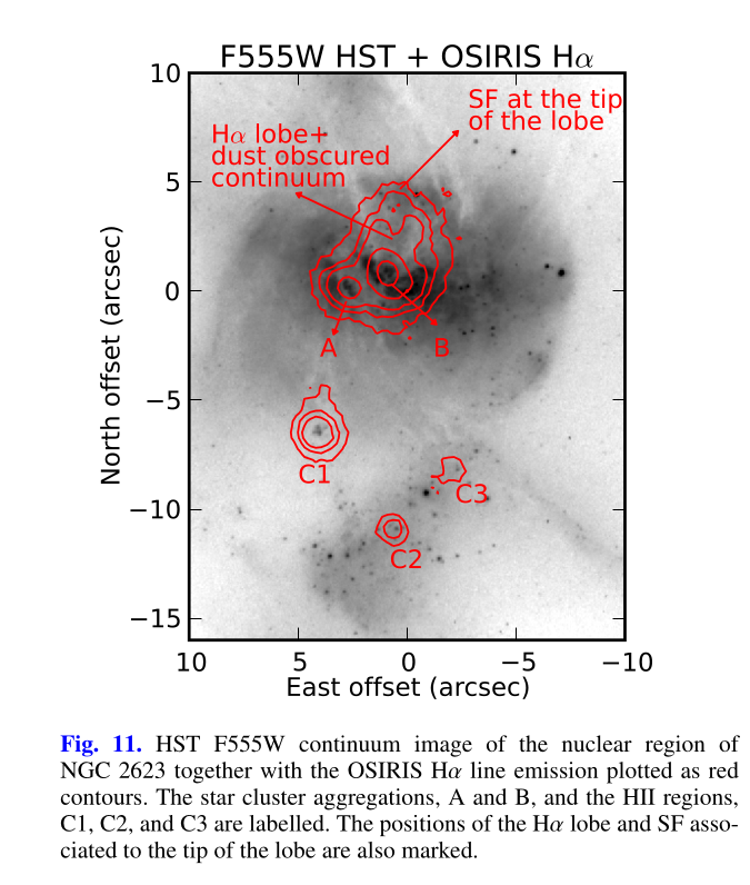
There are several distinct regions of interest, and I’ve taken the liberty of grabbing a screenshot from a figure in Cortijo-Ferrero et al. (2017) for orientation. The central region generally outlined by the Hα contour lines has the highest stellar mass density and ongoing star formation. The 3 H II regions marked C1, C2, and C3 are clearly seen in the emission line maps in my previous posts.

The wedge shaped region in the south that looks relatively blue in optical wavelength color images will turn out to be especially interesting. In the merger models of Privon, Barnes et al. (2013) the material in what Mulia, Chandar, and Whitmore (2015) call the “pie wedge” belongs to the progenitor that formed the northeastern tidal tail and constitutes the base of the tail that is now falling back into the main body of the merger remnant. As we will see the wedge contains most of the post starburst regions in the galaxy. There are also post starburst regions in a chain of bright clumps mostly west and north of the nucleus.

Screenshot of HST image of NGC 2623 with Hα contours overlaid from Cortijo-Ferrero et al. 2017.

There have been a number of attempts to characterize the stellar populations of this galaxy. In a probably non-exhaustive literature review I found 4 that used HST multiband imaging and aperture photometry to estimate the ages of clusters in the tidal tails and wedge: Evans et al. 2008, the aforementioned Mulia, Chandar and Whitmore 2015, Linden et al. 2017, and Cortijo-Ferrero et al. 2017. All of these used broad band color-color diagrams and various versions of BC03 SSP models for age estimates, which is evidently not very precise and highly degenerate with dust reddening. Fortunately the pie wedge region has very low attenuation in my models (τ_V ≲ 0.25). Nevertheless there’s a wide range of estimates in these works. Evans estimated ages of ~1-100 Myr for clusters in the pie wedge. Mulia also found ages of ~100 Myr, claiming that much of the observed scatter was due to photometric errors. They also estimated the age of the diffuse light, finding a somewhat older age of ~500Myr. Linden et al. found a wide range of ages from 3.5-350Myr in just 11 clusters in the pie wedge and the bright clumps west of the nucleus. In an appendix to their mostly CALIFA based study Cortijo-Ferrero used archival HST images to estimate cluster ages to the south of the nucleus in the range 100-400 Myr, with an average ~250 Myr.

There have been 4 IFU based spectroscopic studies that I have found. The study by Lipari et al. that I discussed in the previous two posts exclusively considered emission line properties. Medling et al. (2014) performed a near IR study using an instrument named OSIRIS primarily directed at stellar and gas kinematics. The spatial coverage of their observations was only ~500pc, which is smaller than a MaNGA fiber so their work is not directly relevant. One interesting result is they found the nuclear stellar population to have a mean age ~30Myr.

I already mentioned the CALIFA based study of Cortijo-Ferrero et al. A second paper in the series (Cortijo-Ferrero et al. 2017) performed a comparative study of several (U)LIRGs. Their work is the most similar in objectives and to some extent methodology to mine. I’ve only found two studies concerning stellar population properties using MaNGA observations. Kauffmann et al. (2024) found strong evidence for a population of Wolf-Rayet stars in the circumnuclear region, which would prove the presence of a recent or ongoing nuclear starburst. As I mentioned a few posts ago this was a candidate “Central Post Starburst Galaxy” in the work by Leung et al. For reasons that I may get around to discussing later they chose not to analyze it as part of their final sample.

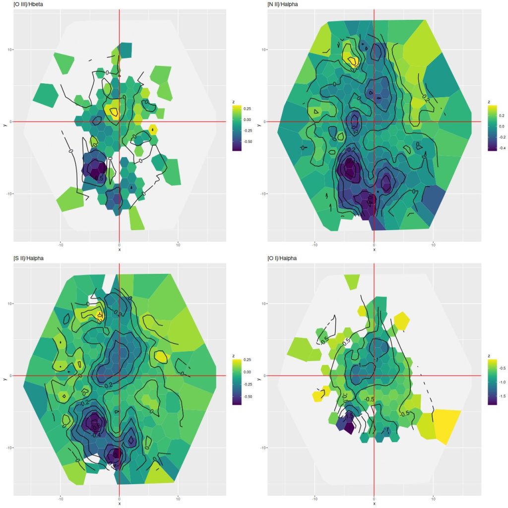
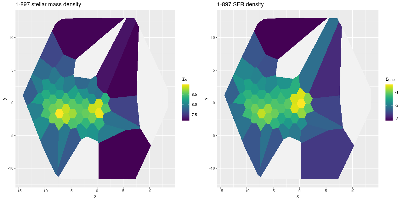
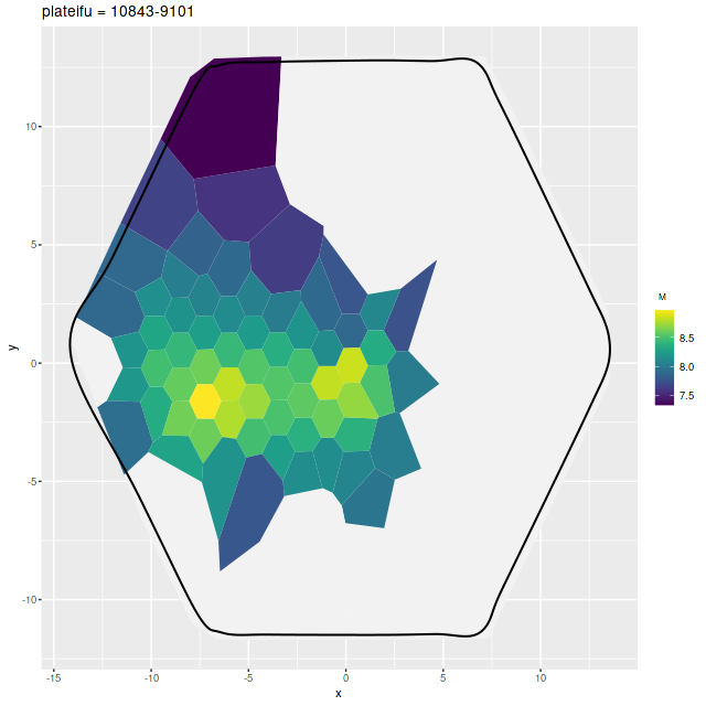
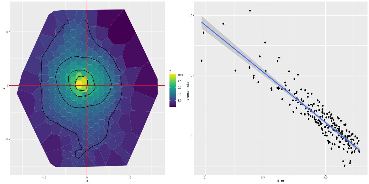
Turning to my own model results I’ll first look at some large scale properties, in no particular order. The stellar mass density peaks just to the east of the nucleus, approximately at the position of the cluster aggregation marked “A” in the HST based image above. The trend with radius appears to be close to exponential, suggesting this system is still disky.

NGC 2623 (MaNGA plateifu 9507-12704) – (L) map of model stellar mass density/ (R) Stellar mass density vs. distance from nucleus

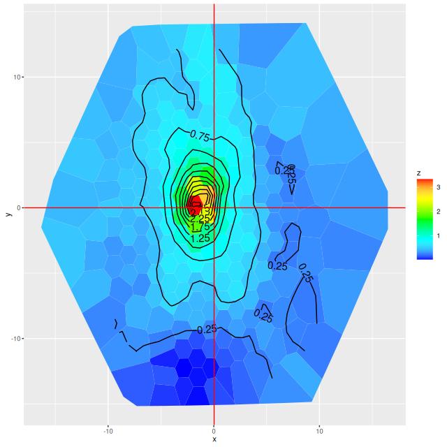
The stellar dust attenuation also peaks just east of the nucleus. Given the complex dust geometry it’s possible my simple one component attenuation model is failing here: if the light is dominated by young stars still in their “birth cocoons” and the model fits the attenuation to them it will tend to overestimate the mass in older stars. This may be a case where I’d be justified in running a model with two dust components.

In the south the area of the pie wedge has mostly very low attenuation, as do the bright clumps south and west of the nucleus.

NGC 2623 (MaNGA plateifu 9507-12704) – Model stellar attenuation

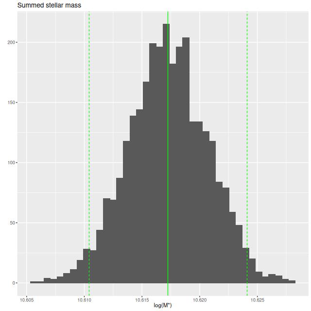
I estimate the total stellar mass within the IFU to be ≈ 4×10¹⁰ M_☉ (log(M*) = 10.617 ± 0.007¹. This is just a sum over all individual estimates, which should overstimate the total by about 0.2 dex since the fiber positions overlap. However the IFU doesn’t quite cover the full visible extent of the main body and almost none of the tidal tails, which will add perhaps a similar amount to the total. This estimate appears within the range I’ve found in the literature. For example Shangguan et al. (2019) give an estimate of log(M*} = 10.60 ± 0.2 (for future reference they estimate the star formation rate to be log(SFR) = 1.62 ± 0.04). The previously cited Cortijo-Ferrero et al. (2017) estimate it to be 2.4 x 10¹⁰ M_☉ with Chabrier IMF. Howell et al. (2010) estimated the stellar mass as 6.42×10¹⁰ M_☉ (log(M*) = 10.81) and the star formation rate at 69.19 M_☉/yr based on IR/UV photometry. The NASA Sloan Atlas catalog, which serves as the source for derived quantities in the MaNGA DRP estimates the stellar mass to be 3.1 – 3.4×10¹⁰ M_☉.

NGC 2623 (MaNGA plateifu 9507-12704) – Total stellar mass within IFU.

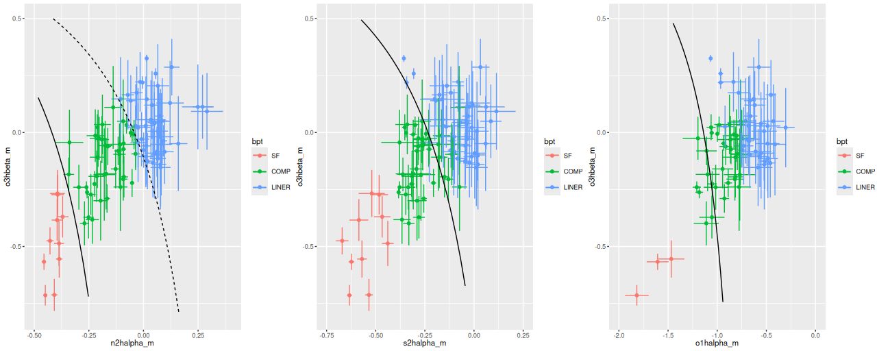
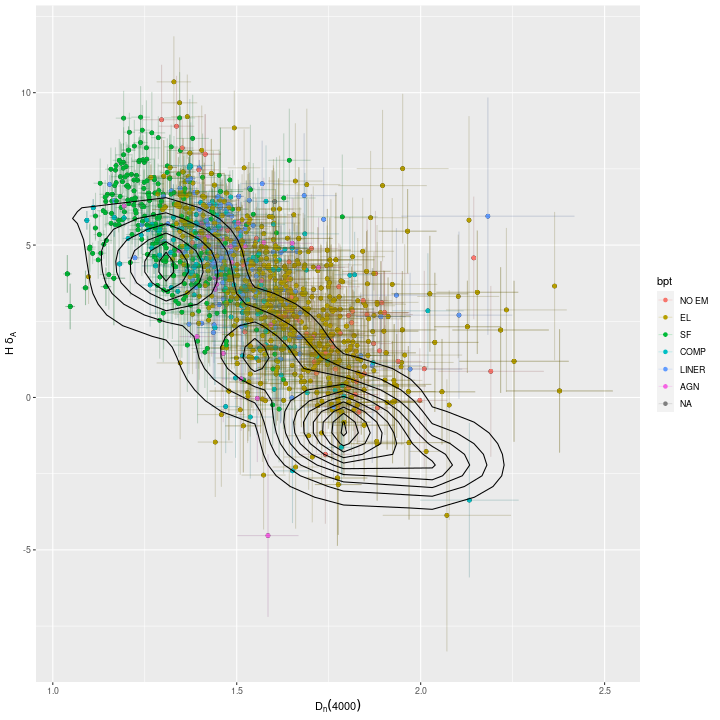
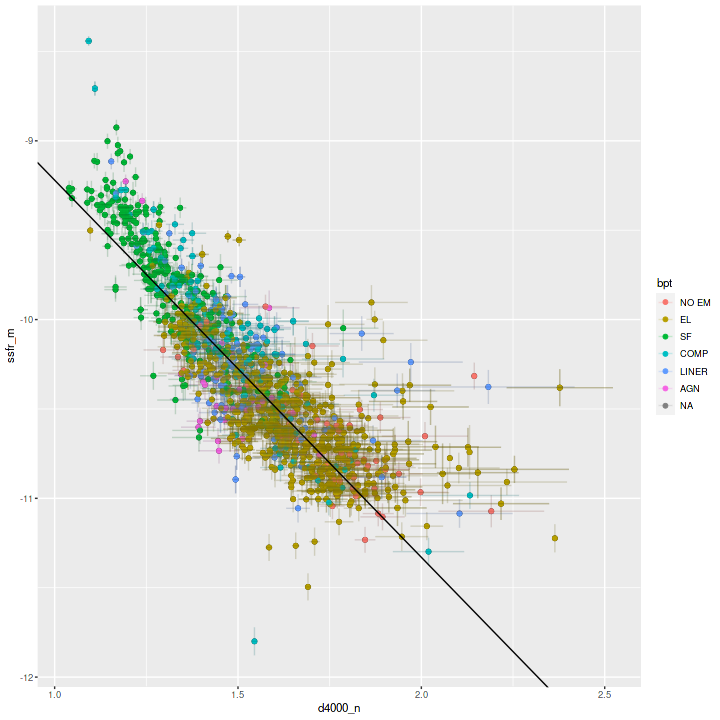
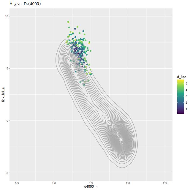
A popular absorption line diagnostic, and one I’ve displayed several times, is a plot of Balmer line strength versus the 4000Å break strength. Although it doesn’t uniquely constrain the evolutionary state of a system it does give some rough idea of the contribution of intermediate mass stars and the mean stellar population age. Plotted below are the Lick Hδ_A index and D_n(4000). The contour lines are for a large fraction of SDSS galaxies measured by the MPA-JHU pipeline. Note that many of the points are above the last contour line in the region, which indicates a significant fraction of the galaxy is in a post-starburst state.

NGC 2623 (MaNGA plateifu 9507-12704) – plot of H&delta_A versus 4000Å strength D_n(4000).

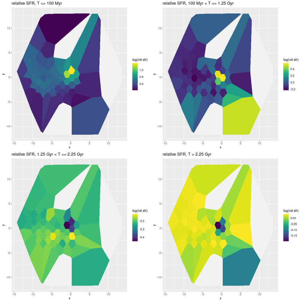
Part of my post-processing of models are calculations of star formation rate surface densities log₁₀(Σ_SFR) in units of M_☉/yr/kpc² averaged over a preselected lookback time interval. I’ve always used 100Myr as that interval, mostly because it’s a nice round number that’s often used in the literature. This time I decided to do also a calculation for a 10Myr lookback time, which is about the timescale for estimates based on Hα luminosity. The results are shown below: the top row are the estimates, and the difference is in the bottom left. As can be seen in the scatterplot at bottom right a small region near and just east of the center has had a recent increase in star formation, while it’s remained nearly constant out to about 1.5 kpc (~ 1/2 r_eff) and has declined farther out.

NGC 2623 (MaNGA plateifu 9507-12704) –
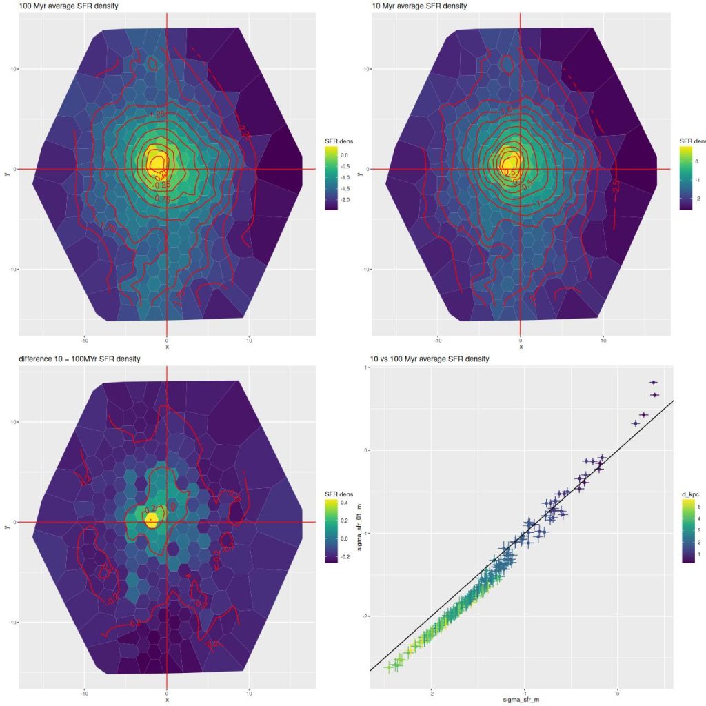
Top row – model mean star formation rate density averaged over 100 and 10 Myr intervals (logarithmically scaled). Bottom left: difference between 10 and 100 Myr averages. Bottom right: scatter plot of 10Myr SFR density vs. 100Myr.

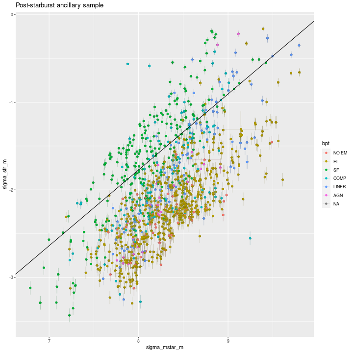
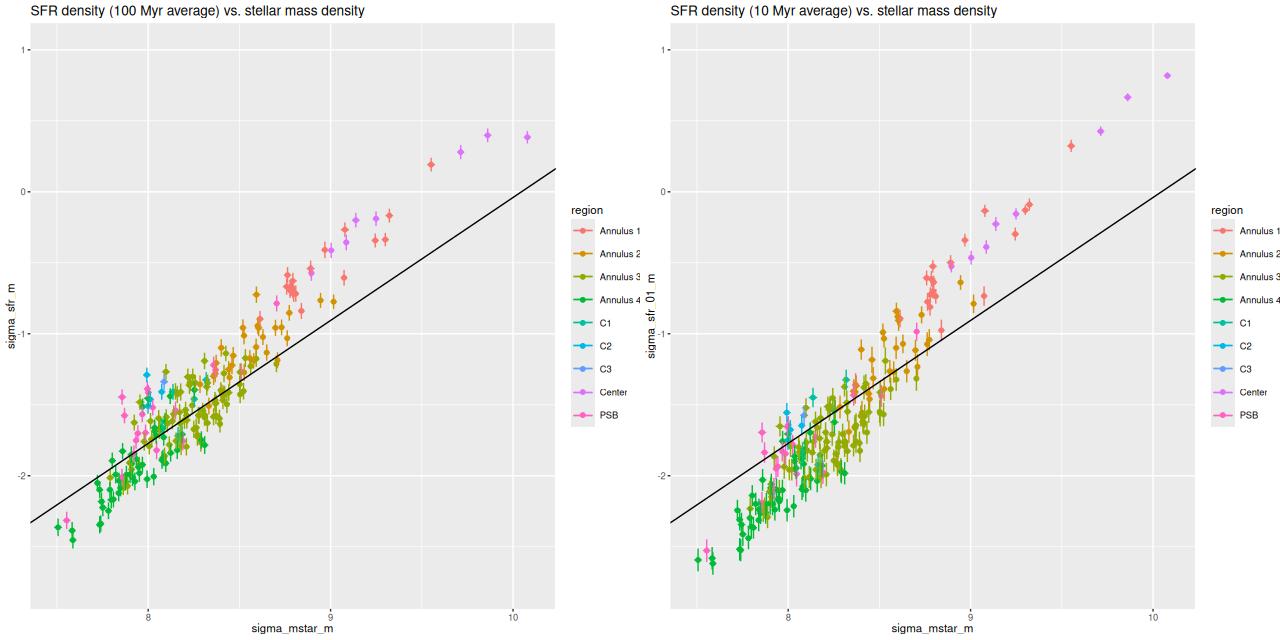
Finally, here is another standard visualization of the relation between star formation rate density and stellar mass density. The left panel is the 100 Myr averaged SFR density while the right is 10 Myr. The straight line is my estimate of the mean “spatially resolved star forming main sequence.” This was done some time ago with a sample of normal starforming disk galaxies and the EMILES + Pypopstar SSP library and should probably be recalibrated. Comparing the two plots it’s apparent that some regions are evolving into the “green valley” while others have evolved into the starbursting region.

NGC 2623 (MaNGA plateifu 9507-12704) – SFR density vs. stellar mass density. (L) 100 Myr average. (R) 10 Myr average SFR density. Straight line is my estimate of the “spatically resolved star forming main sequence.”

Star formation rate histories by region

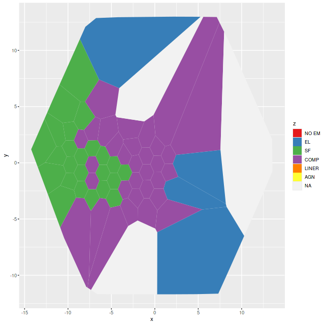
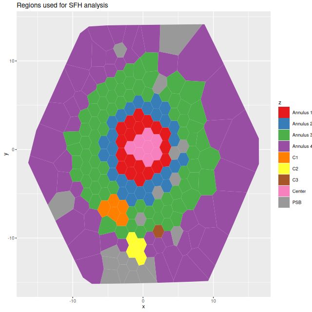
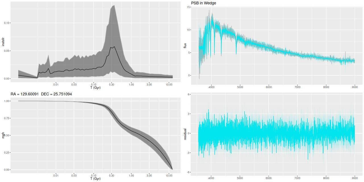
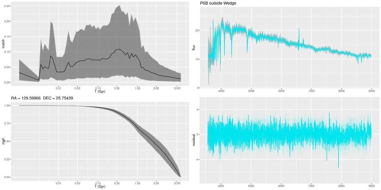
I’m now, finally, going to present detailed star formation rate histories for the entire IFU footprint. The stacked RSS spectra binned to 214 with SNR ≥ 8.5, which is a few too many to display individually. As we’ve seen there are at least 3 distinct regions with likely different recent star formation histories: the circumnuclear region has a central starburst and at least two large star cluster complexes; farther out there are 3 separate areas with star forming emission line ratios and enhanced Hα fluxes relative to their surroundings; the “pie wedge” has many star clusters with estimated ages ~100Myr and post-starburst spectra. Some of the bright clumps seen to the west of the nucleus also have post-starburst spectra. For display purposes I’ve made a slightly finer grade division as follows:

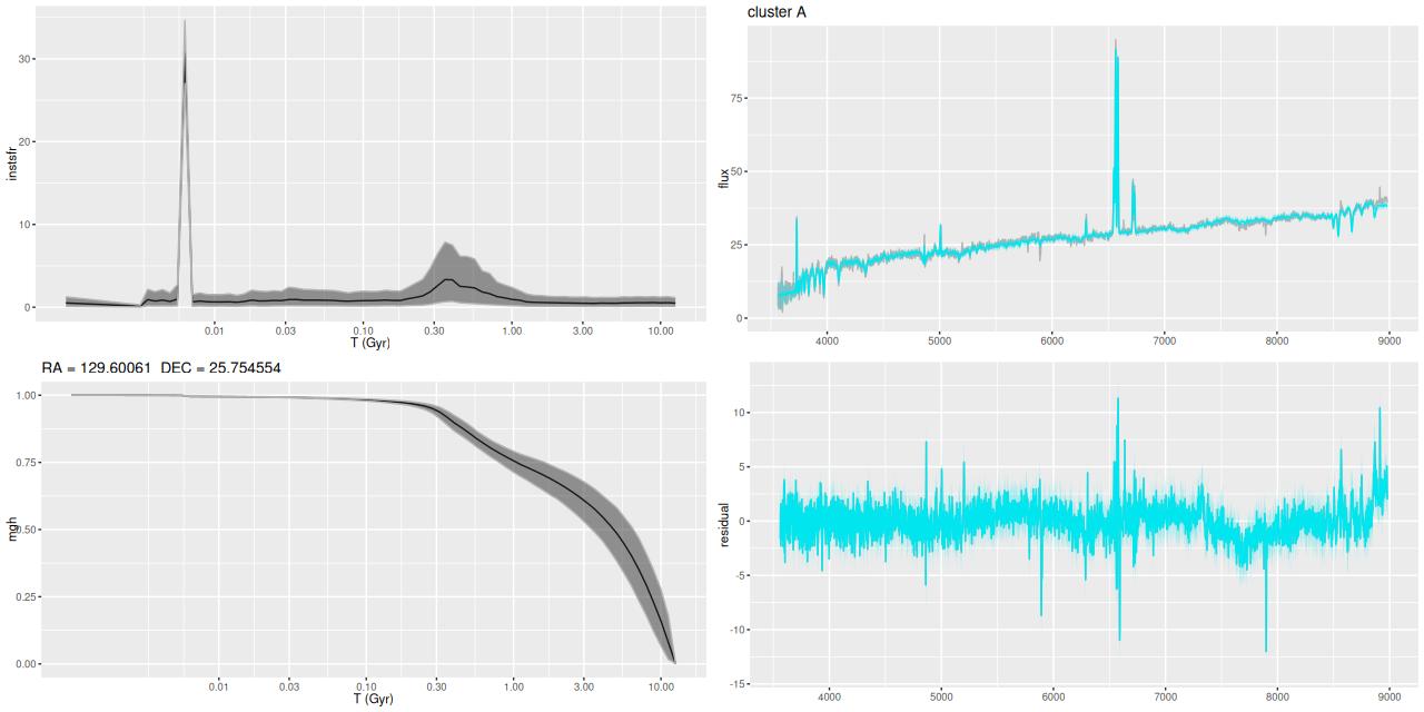
Center region: the closest fiber to the center and its immediate neighbors including cluster aggregation “A” to the east. (see top of post). This covers most of the region with highest emission line flux.
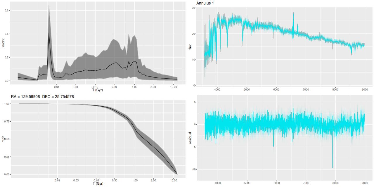
Annulus 1: regions with D ≤ 0,5 r_eff (I adopted r_eff = 7.9″ ≈ 2.9 kpc from the NSA atlas) and outside the center region.
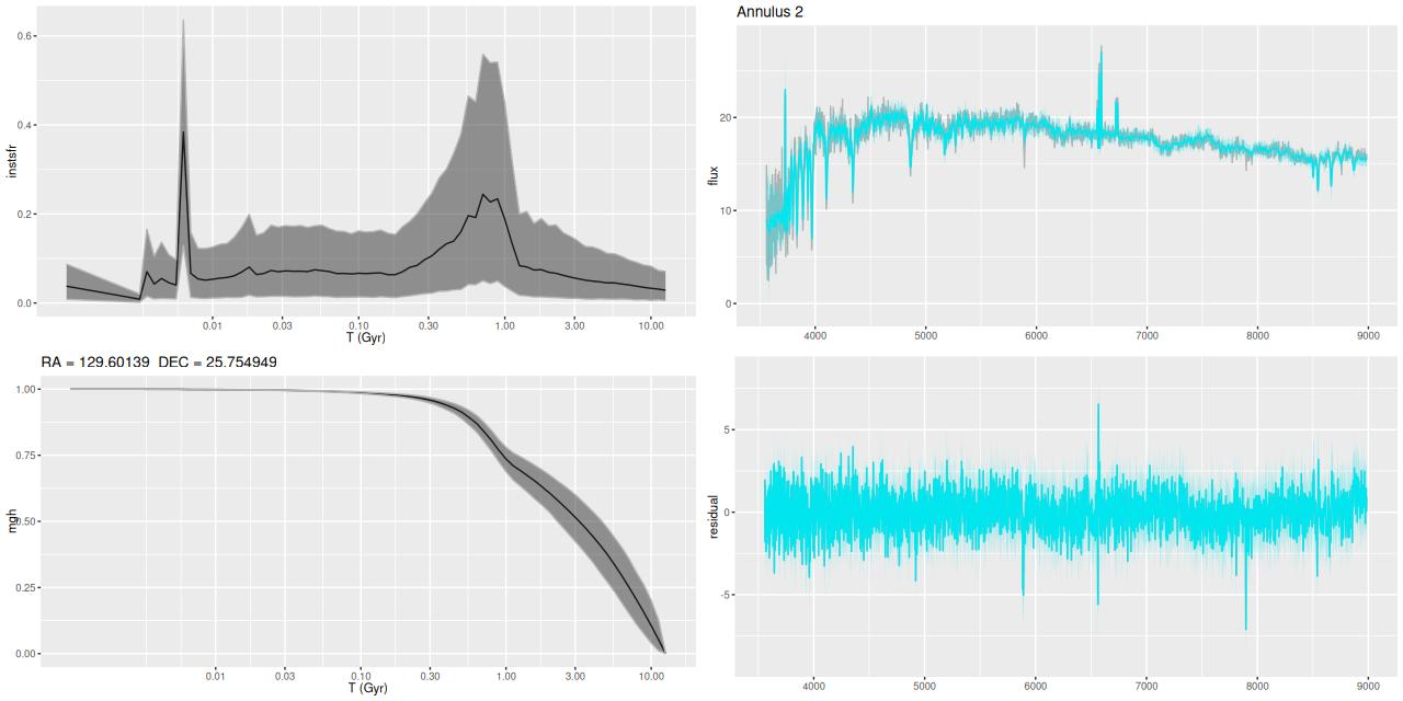
Annulus 2: 0.5r_eff < D ≤ 0,75 r_eff, excluding regions with post-starburst spectra.
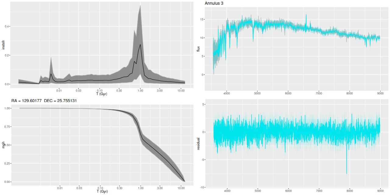
Annulus 3: 0.75r_eff < D ≤ 1.25 r_eff, excluding regions with post-starburst or starforming spectra.
Annulus 4: D > 1.25 r_eff, excluding regions with post-starburst or starforming spectra. The maximum IFU coverage is 2r_eff.
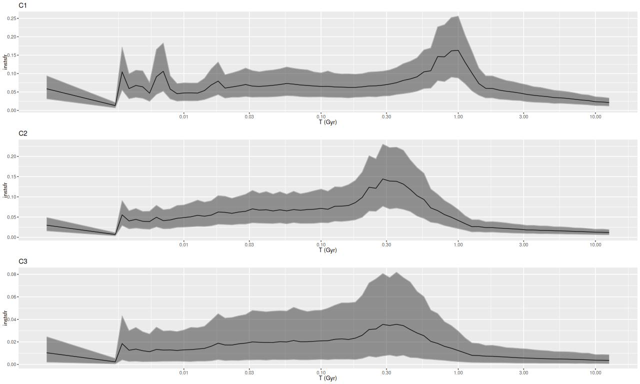
I chose to display the 3 regions of H II aggregations separately. The first is the one labelled “C1” in the graphic at the top of the post.
H II region(s) “C2”
H II region(s) “C3”. Both of these lie at the edge of the “pie wedge.”
Visual examination of the spectra showed that many of them have classic A+K like spectra, with very strong Balmer absorption and weak emission (this was known some years ago: see Liu and Kennicutt 1995). I made a PSB region selection with highly stringent criteria:
- Lick Hδ_A – 2σ(Hδ_A) ≥ 6.25Å
- BPT class of “EL” or “NO EM” (i.e. weak or no emission lines detected). I used this instead of the more traditional equivalent width criterion mostly because I haven’t validated my EW calculations.

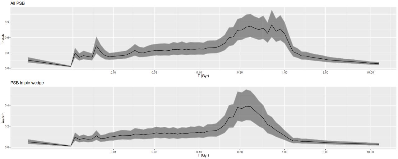
Essentially all of the “pie wedge” meets these criteria, as do several bright clumps west of the nuclear region. With relaxed selection criteria much of the galaxy outside the circumnuclear region could qualify by, for example Alatalo‘s criteria for “Shocked POststarburst Galaxies.”

NGC 2623 (MaNGA plateifu 9507-12704) – Distinct regions used for aggregated SFH model plots. Note that the post starbursts are in several disconnected regions.

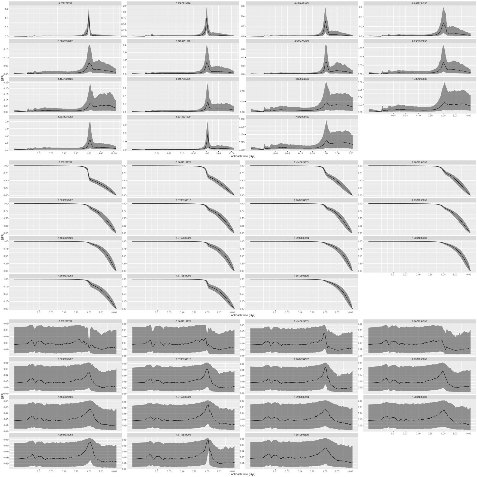
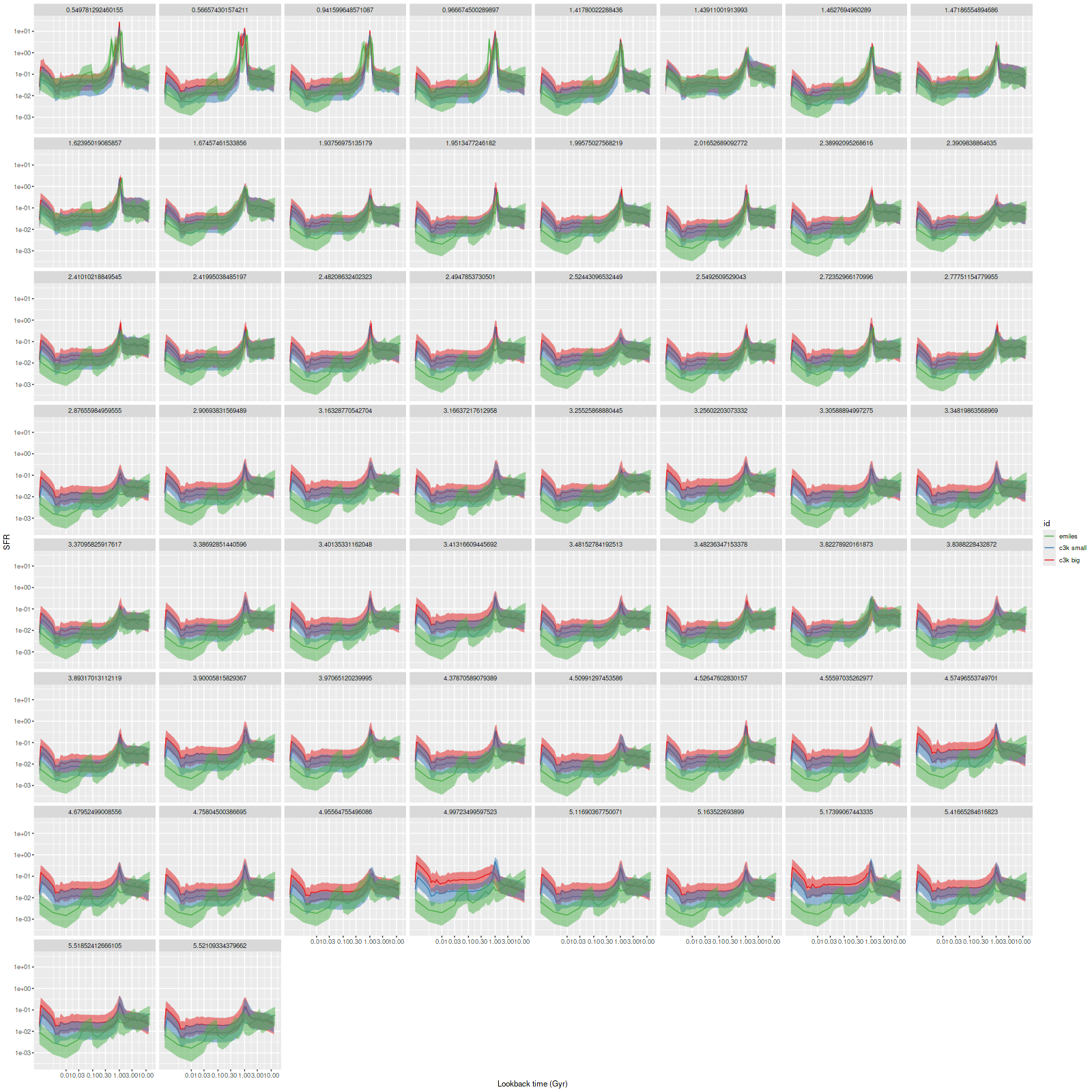
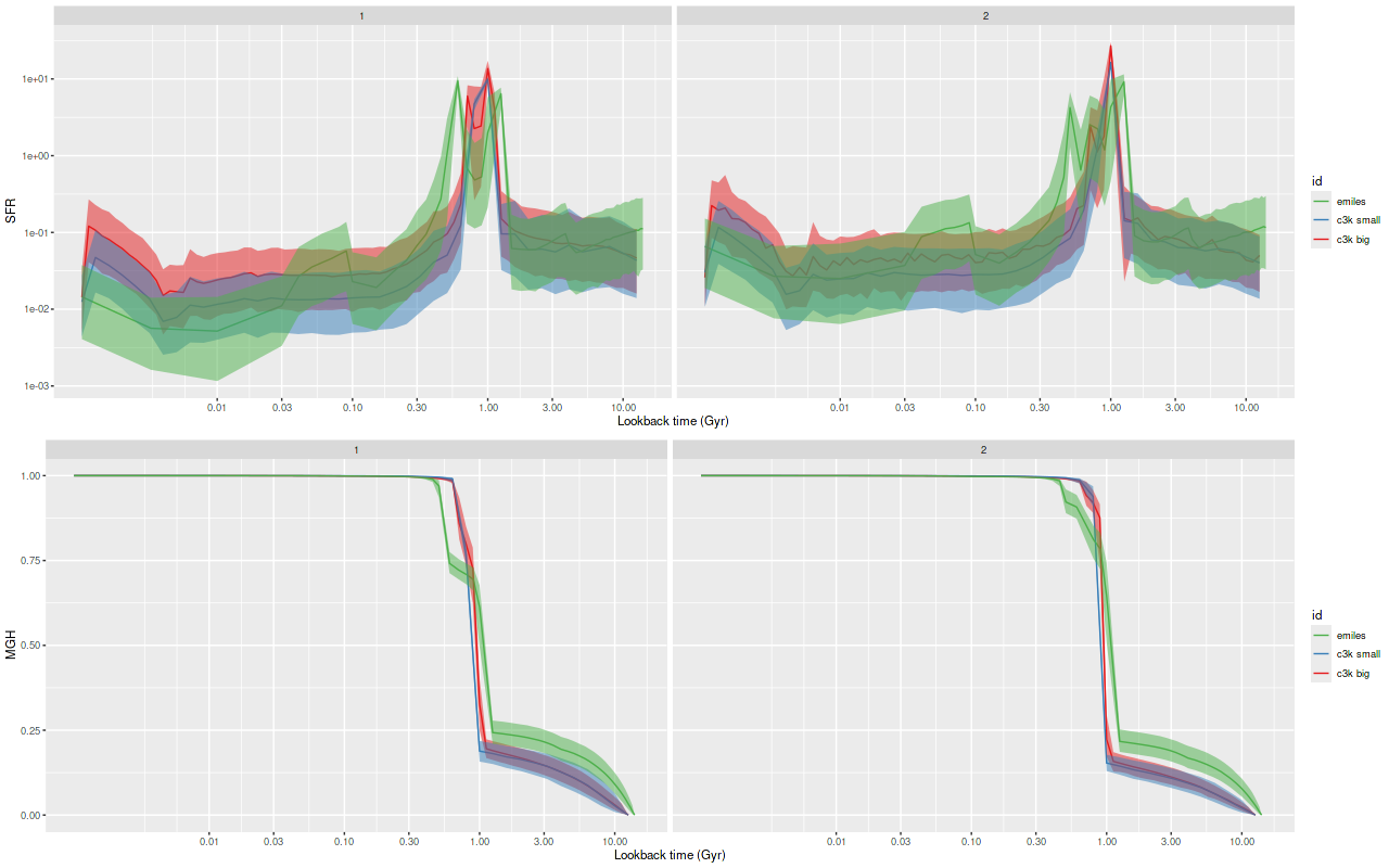
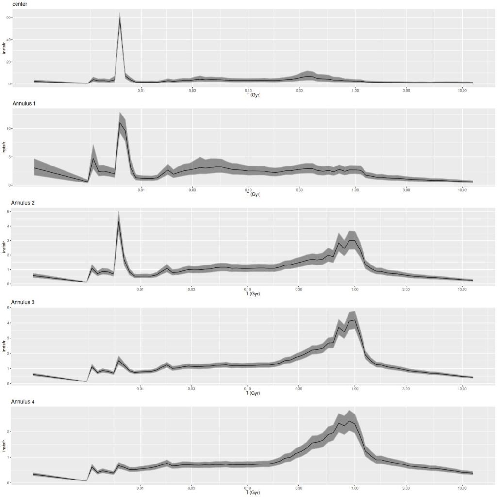
Modeled SFR histories are shown below grouped into 3 sets. The horizontal axes are logarithmically scaled, while the vertical axes are linear with different scales for each plot. Units are M_☉/yr; these are estimated by summing over all models for the binned spectra comprising each group.

SFH in annuli

Star forming regions

Post starburst regions and the “pie wedge”

To summarize my visual impressions, star forming appears to have accelerated beginning ≈1 Gyr ago. In what is now the main body of the galaxy it plateaued shortly thereafter and then slowly decayed until very recently (< 10 Myr) where we are seeing a centrally concentrated starburst with declining star formation in the outskirts of the main body.

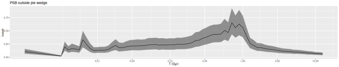
In the pie wedge including the two starforming regions the peak was much later at ≈300 Myr, and again with a subsequent slow decay. The only difference between the starforming and PSB regions of the wedge is the former evidently still have enough residual star formation to power H II regions. The PSB regions outside the pie wedge have a much different SF history from those inside it, with an early peak at ~1 Gyr and slow decay, much like the rest of the galaxy outside the center. The broad plateau in the first of the PSB plots is therefore a bit of an illusion.

Although it’s obscured by the current starburst the central region also had a peak at ≈300 Myr.

NGC 2623 (MaNGA plateifu 9507-12704) – model star formation history in central region. Logarithmically scaled SFR

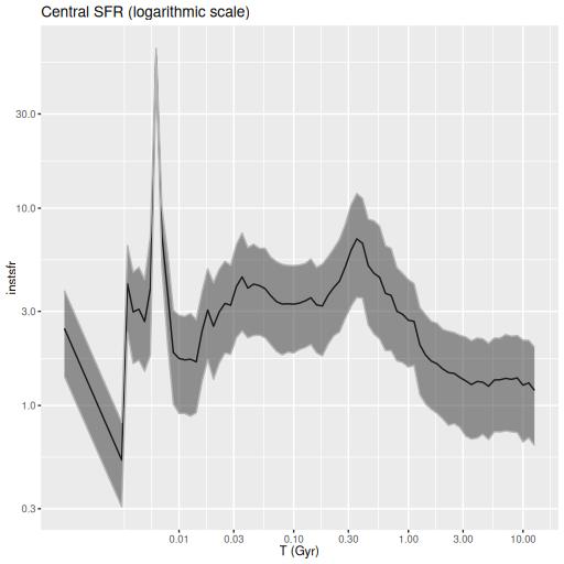
The 300 Myr peak is consistent with Privon et al.’s estimate of a first pericenter passage at ~220 Myr ago as well as the HST based estimates of star cluster ages in the wedge. However coalescence at ~85 Myr ago seems to have had no effect on star formation in my models — this is in contrast to most recent merger simulations, which typically have a strong centrally concentrated starburst around the time of coalescence. The large scale enhancement of SFR beginning at ~1 Gyr is also a bit puzzling. If the model is correct the effects of the interaction began well before the merger was underway.

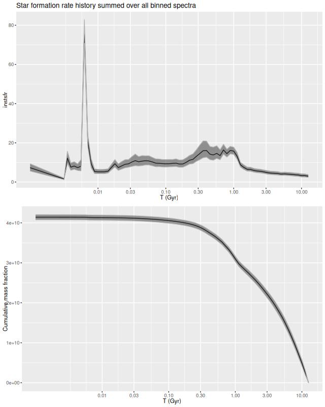
Finally for this section, here is the model star formation history summed over all 214 individual models. System wide there was a broad plateau from ~! Gyr to ~300 Myr ago, with a slow decline until ~10 Myr. The recent starburst only adds about 0.3% to the present day stellar mass, ~10⁸ M_☉.

NGC 2623 (MaNGA plateifu 9507-12704) – Model star formation rate history and mass growth history summed over all models for all binned spectra.

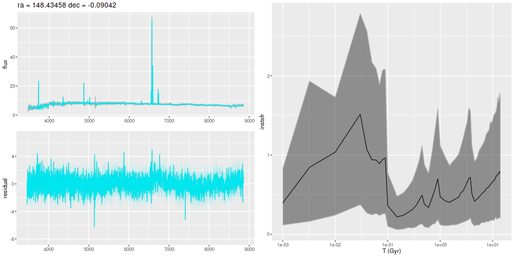
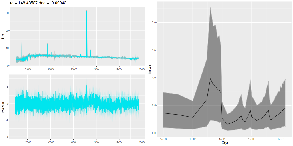
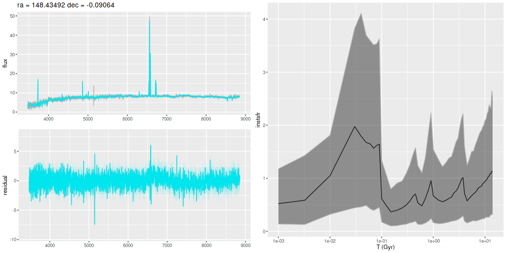
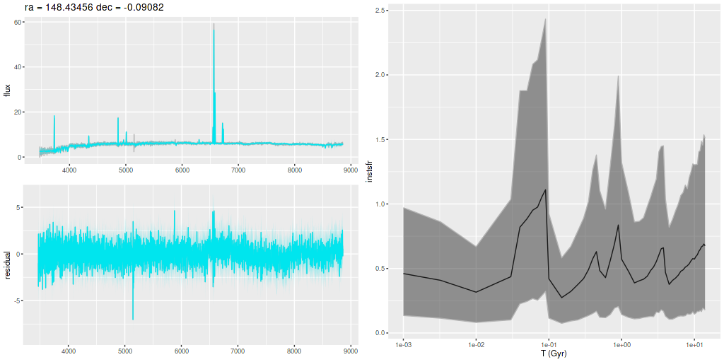
Selected individual SFH models

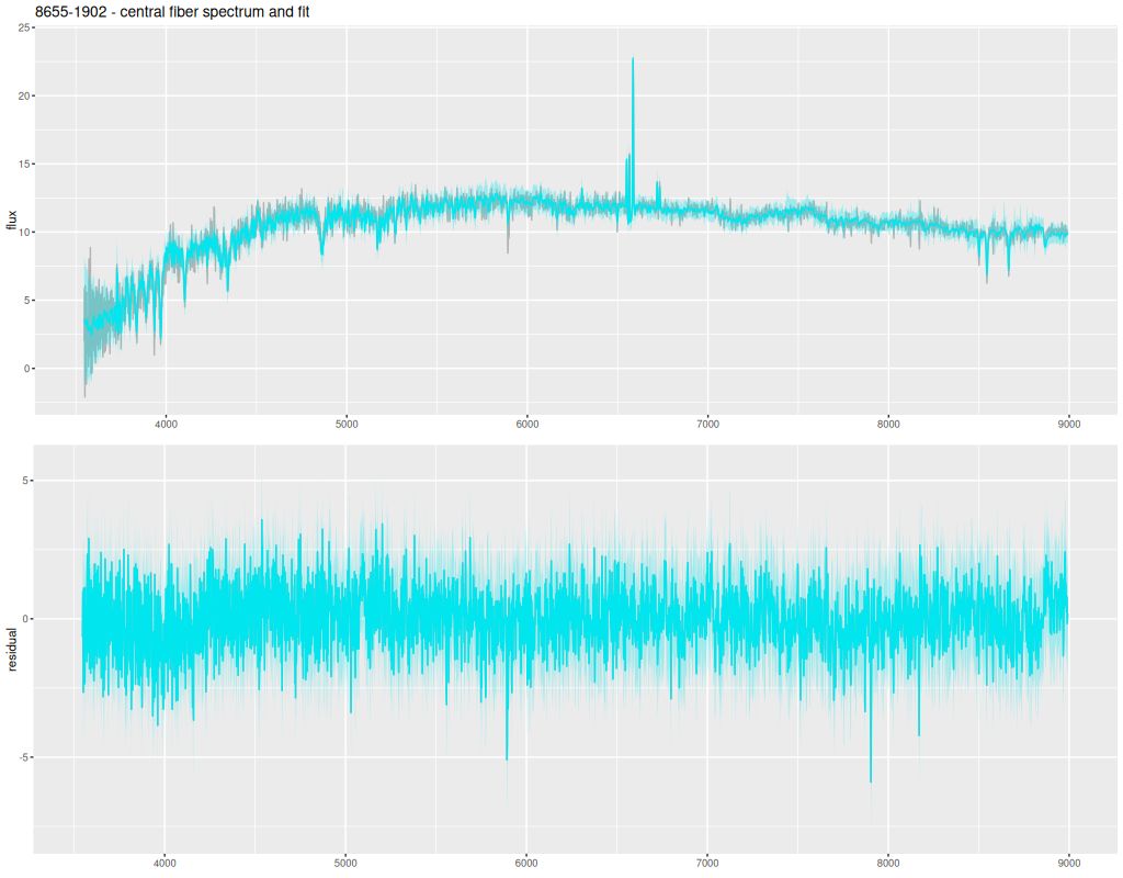
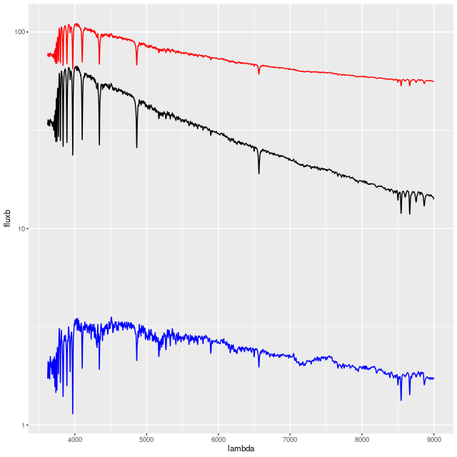
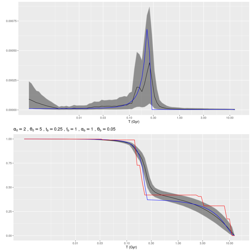
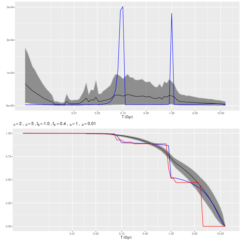
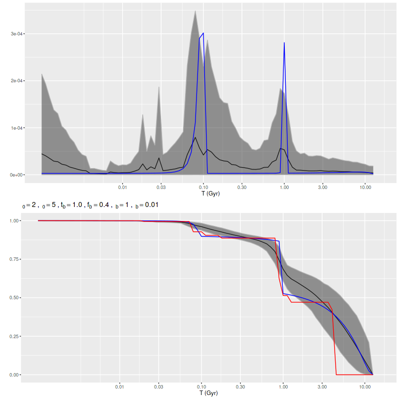
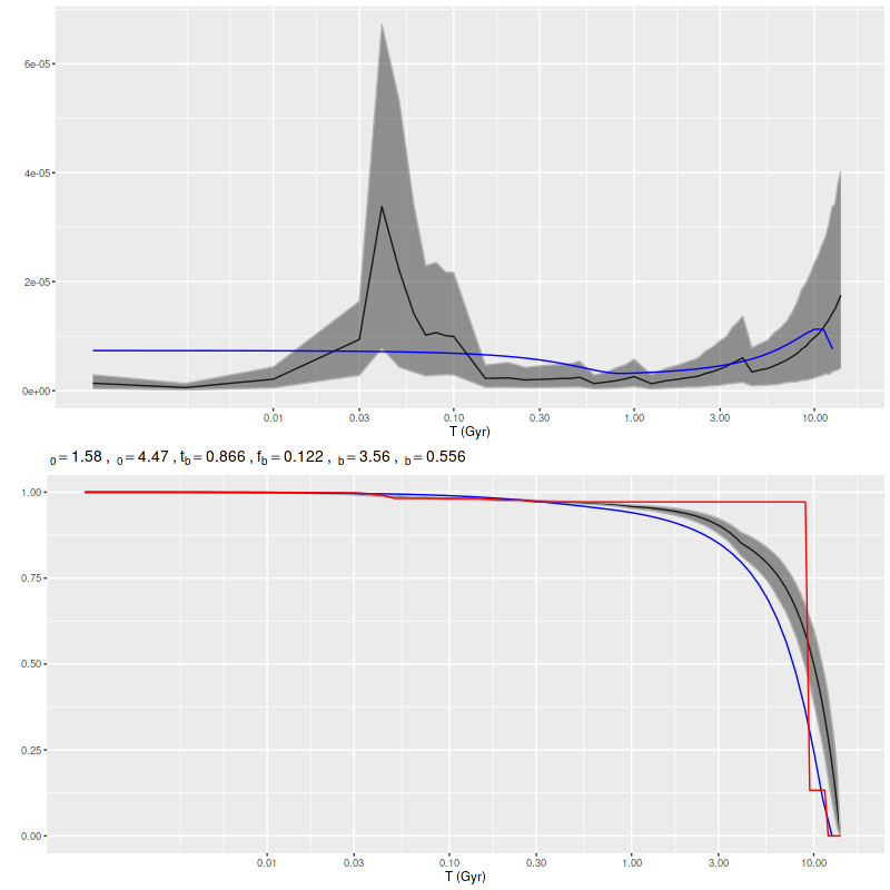
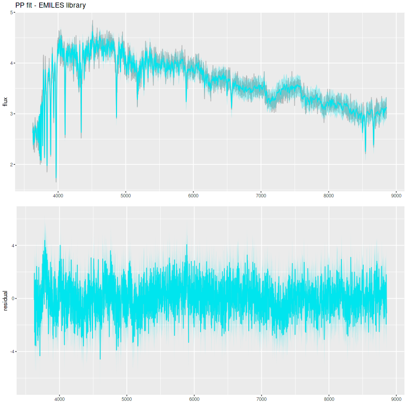
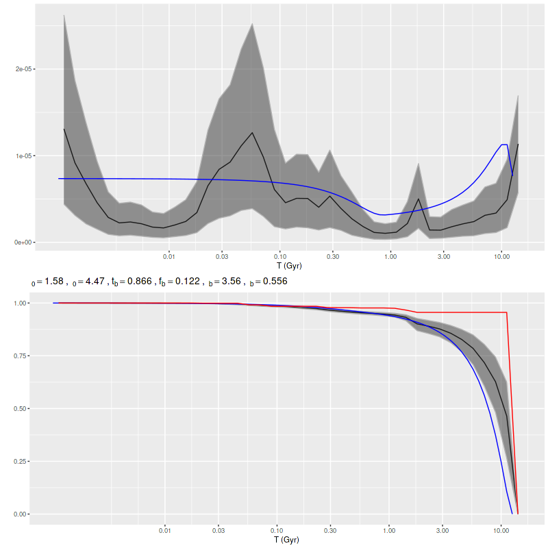
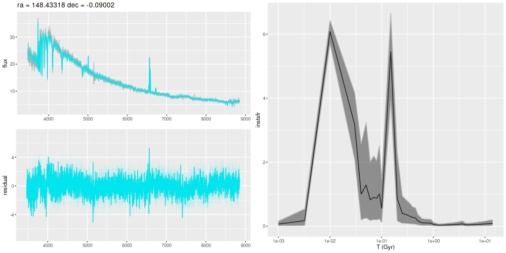
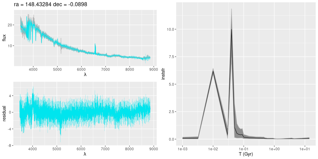
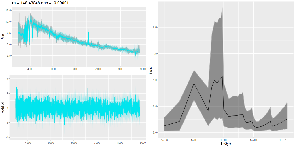
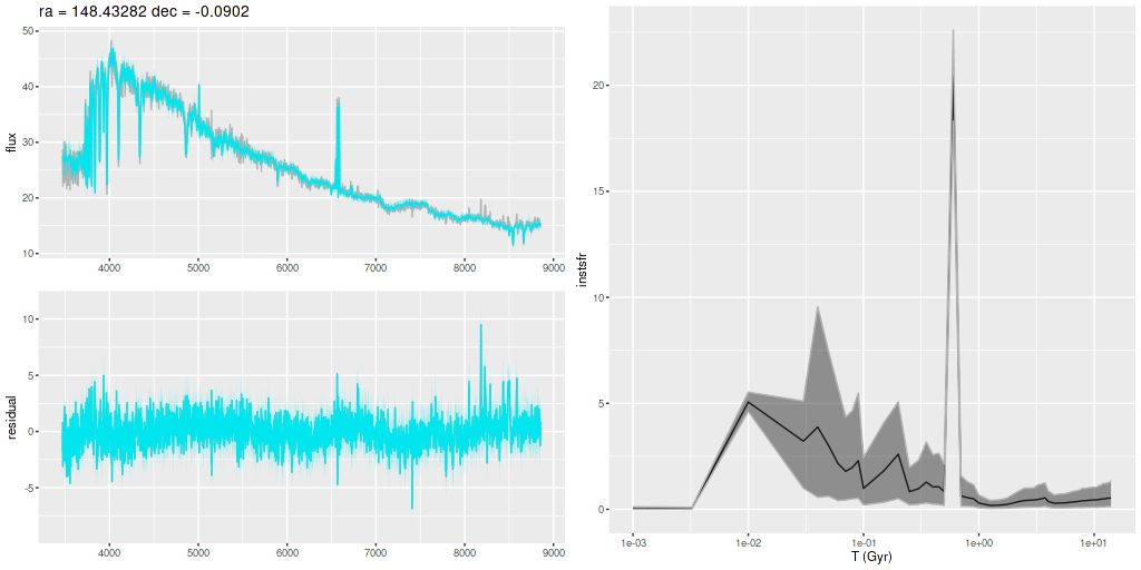
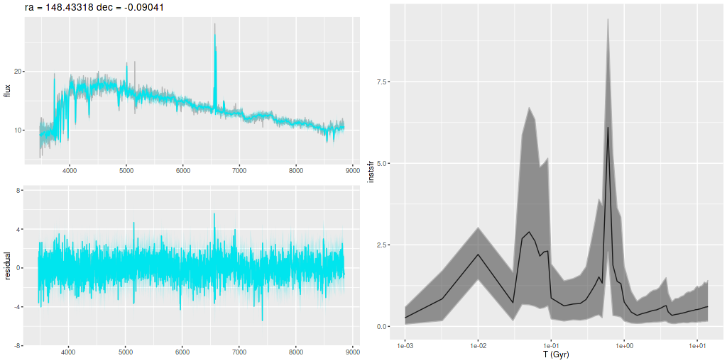
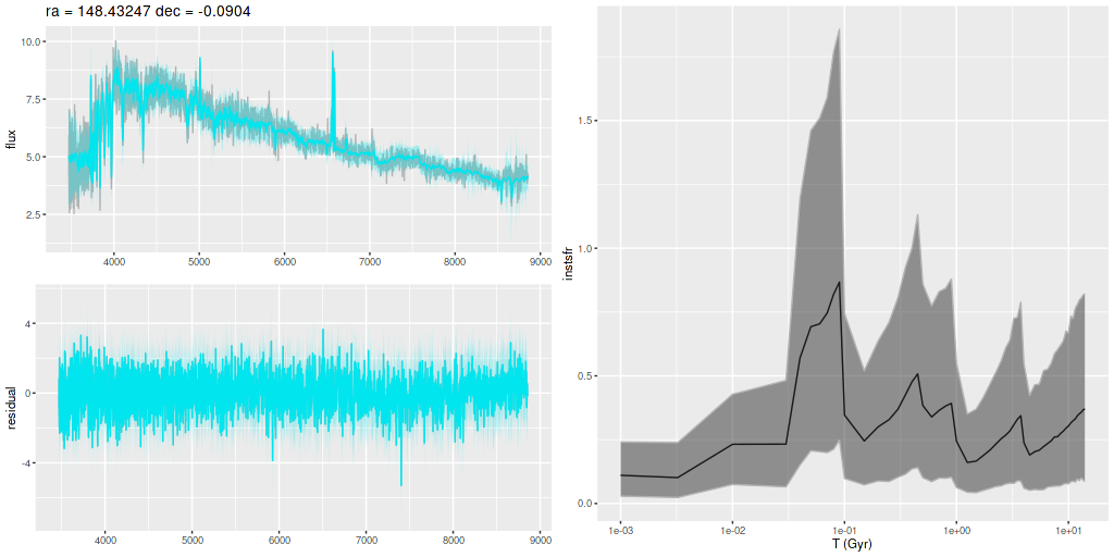
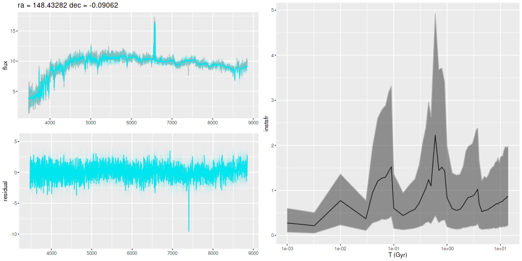
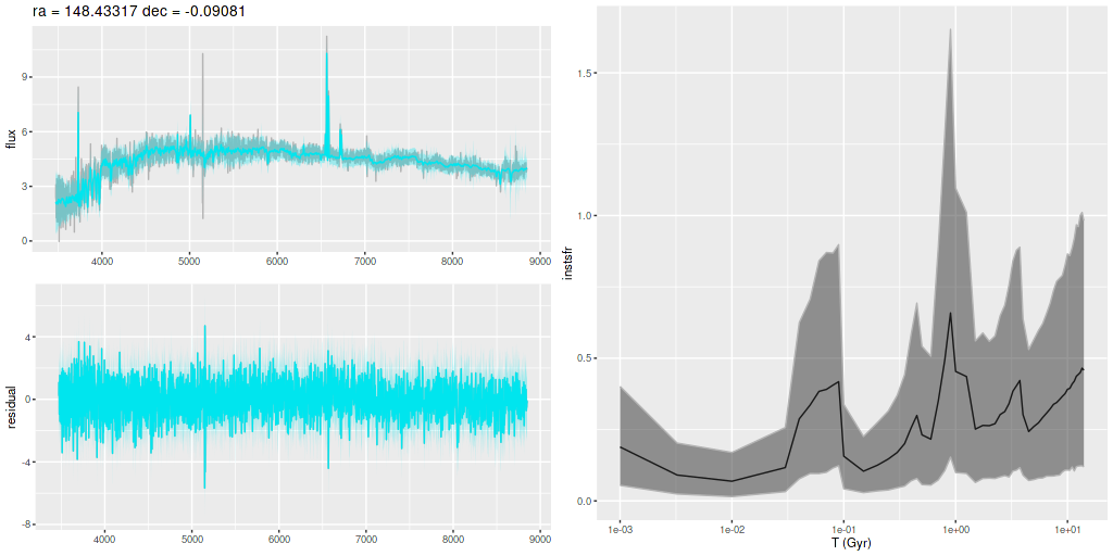
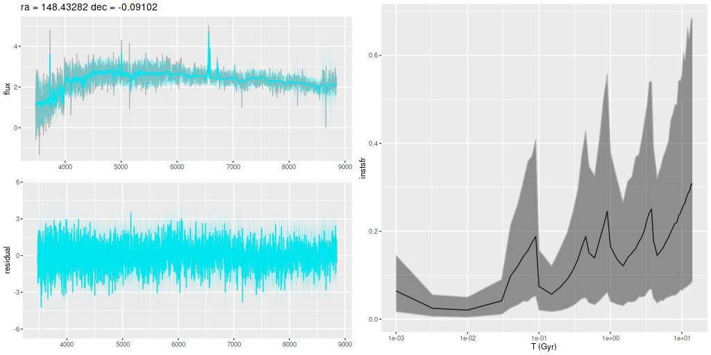
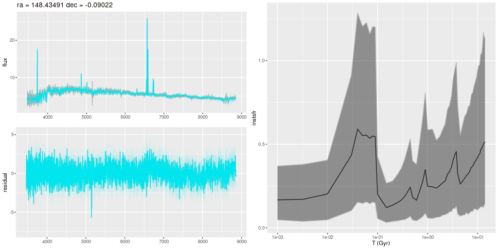
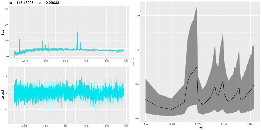
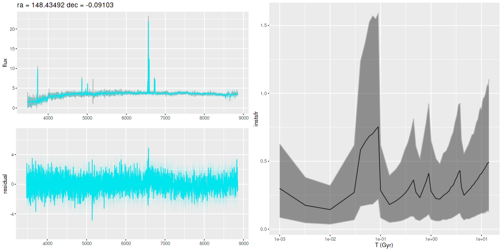
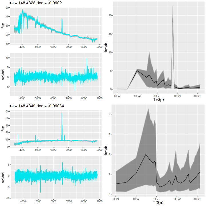
Plotted below are model star formation histories and fits to the data for 13 individual spectra, with the same ordering by region as the previous subsection. All horizontal scales are the same: lookback times are logarithmically scaled in Gyr; wavelengths are rest frame and cover the range of the model fits, which is ≈3560-9000Å. Vertical scales are linear with ranges chosen to cover the values plotted in each model run. The SFH plots include the position of the fiber center.

I picked four regions from the center. First is the fiber closest to the nucleus. One oddity of the RSS files is the central fiber is usually offset from the IFU center, in this case by about 3/4″ to the NW. The IFU center is exactly at the consensus position of the nucleus, and there are two fibers that straddle it. The other one is located just to the SE– notice that it has a much higher peak star formation rate than its immediate neighbor and a considerably redder continuum. The region with the highest 100 Myr average star formation rate is the neighbor to the NE, which is close to the cluster aggregation “B” in the HST image at the top of this post. Finally for the center spectra, the highest 10 Myr averaged SFR density of ≈7 M_☉/yr/kpc² is the region to the east that is centered in a prominent dust lane and includes at least part of cluster complex “A”. It also has the highest model stellar attenuation (τ_V≈3.3) and the highest Hα luminosity density corrected for stellar attenuation.

Fits to the data are somewhat problematic in the center. The non-Gaussian emission line profiles are prominent in the residuals. and there are systematic residuals in the stellar continuum as well. The complex dust geometry and kinematic decoupling of gas and stars are likely contributors to the lack of fit, and there are the usual issues of possibly missing ingredients in the inputs. How much the fit errors affect the SFH models is unknown.

NGC 2623 (MaNGA plateifu 9507-12704) –
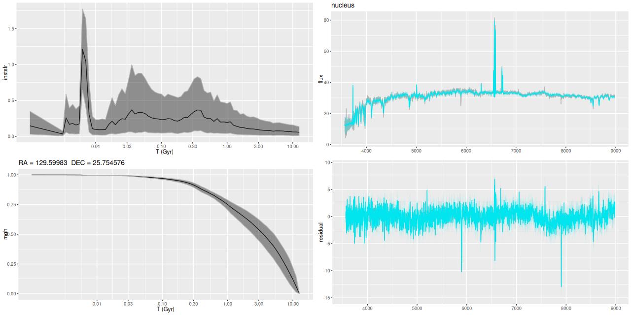
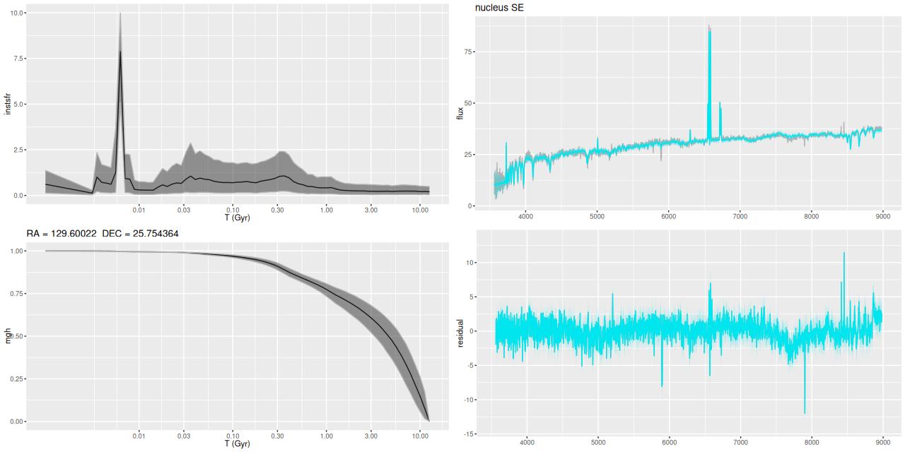
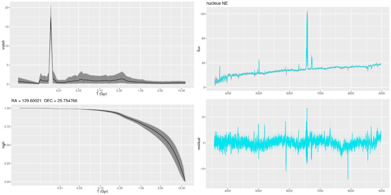
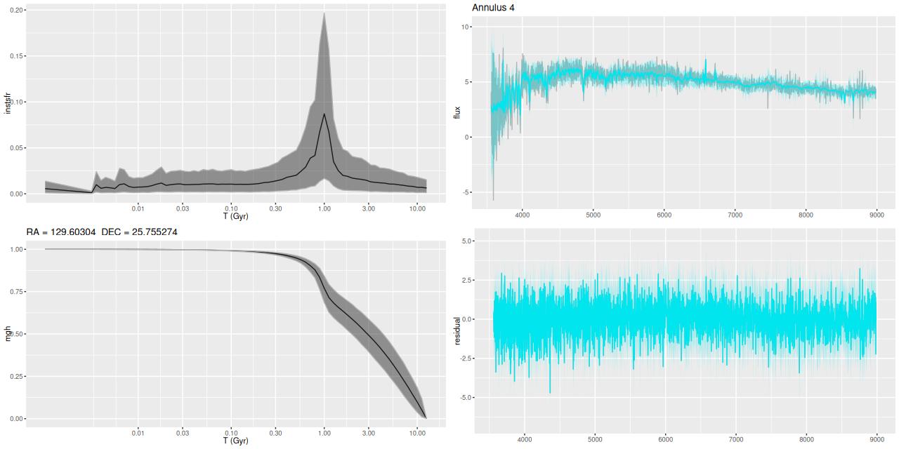
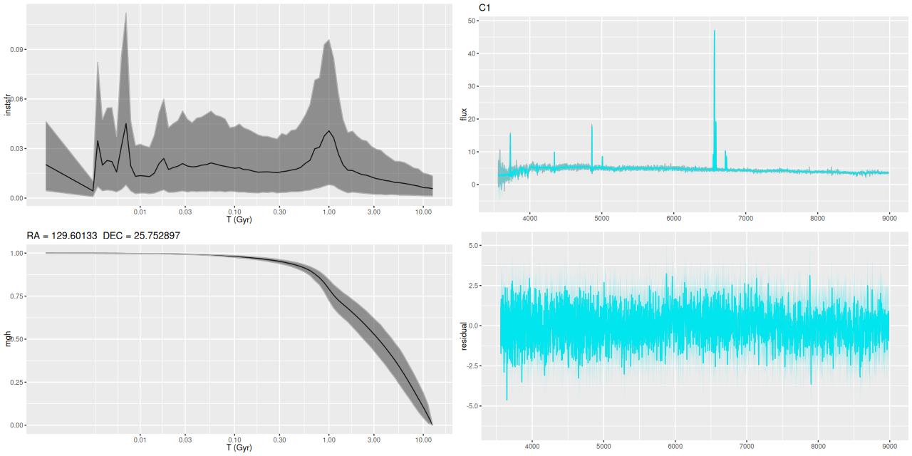
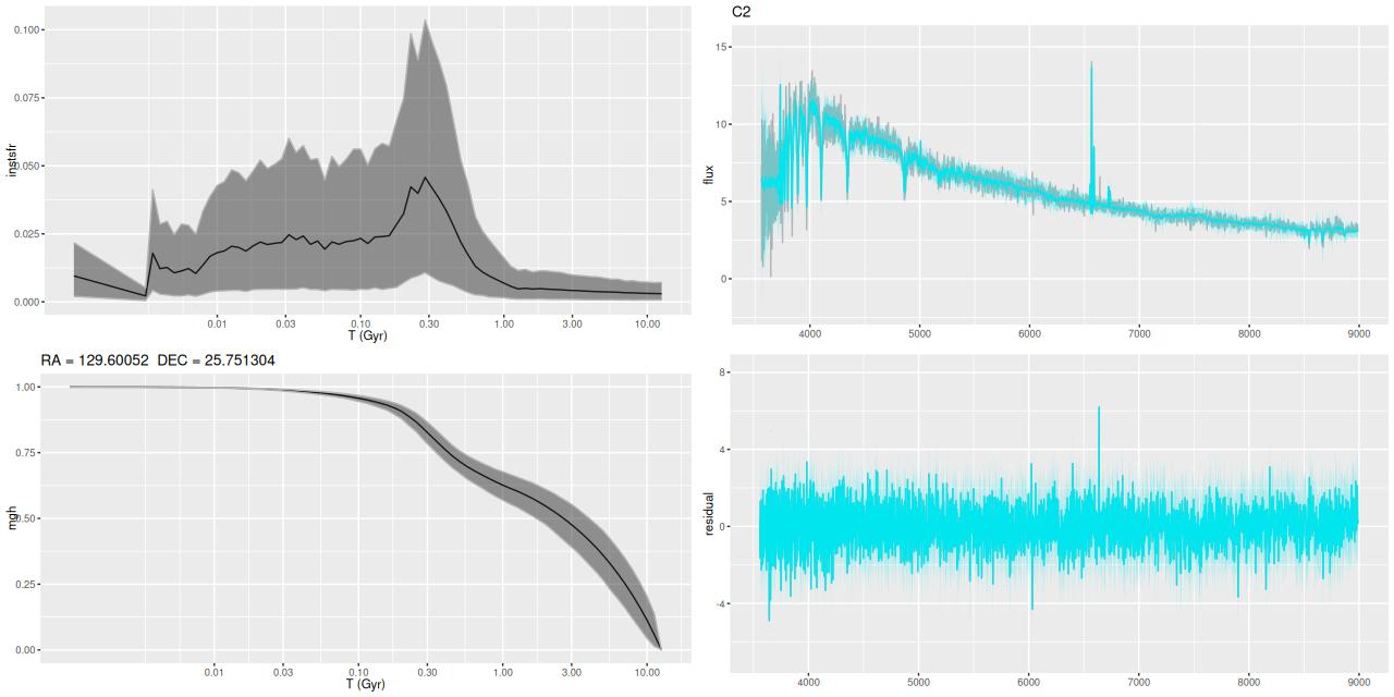
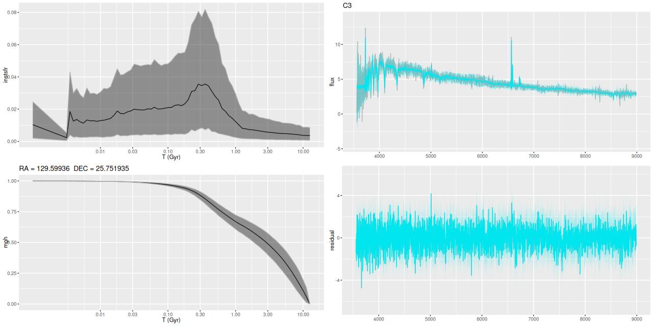
Sample star formation histories and posterior predictive fits to the spectra. Fiber center position and galaxy region are indicated on left and right panels respectively

A brief comparison with Cortijo-Ferrero

As I mentioned previously Cortijo-Ferrero (2017a, 2017b) published two papers studying this galaxy and a small number of other (U)LIRGS using data from CALIFA and a few other instruments. Their objectives in paper (a) were essentially the same as mine in these posts, and their methods were somewhat similar. For spectral fitting they used a code named STARLIGHT, which is not Bayesian and as far as I can tell doesn’t have any convergence guarantees but does perform nonparametric SFH modeling.

The first paper devotes one section apiece to ionized gas properties and stellar populations. Since I’ve discussed the former at some length in my previous posts I won’t review their results in detail. Quantities that I was able to compare agree well. They also found the kinematic center of the gas to be offset 2″ to the east of the nucleus, in agreement with my results and Lipari. They comment that the offset is “within (their) spatial resolution,” which is true but misses the point that the entire rotating structure is much larger and is clearly offset from the nucleus even on visual inspection.

For comparison purposes I’m going to reproduce some of their graphical results. They have maps of many quantities as well but visual comparisons are difficult because they are displayed at postage stamp size in the online journal papers and also because the authors made some truly atrocious choices of color palettes. I’ve already displayed a map of stellar mass surface density and its trend with radius, which can be compared to their figure 4 in paper (a). The values and trends with radius are similar in my models to theirs although I don’t see a break in the relation as shown in their lower plot.

Their model for stellar dust attenuation is similar to mine: they assume a single foreground screen with Calzetti attenuation. I include an additional parameter controlling the overall steepness of the attenuation curve, which essentially amounts to allowing R_Vto be variable. The peak values near the center are considerably higher in my models than theirs (cf figure 5 in paper a). This could be partly due to the slightly higher spatial resolution in MaNGA. More importantly perhaps my models have a “greyer” attenuation curve than Calzetti’s in the center which means a larger attenuation value is required for a given amount of reddening. Farther out there is good agreement.

NGC 2623 (MaNGA plateifu 9507-12704) – Stellar attenuation τ_V vs. radius in half light radii

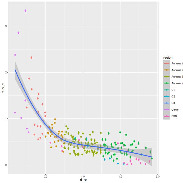
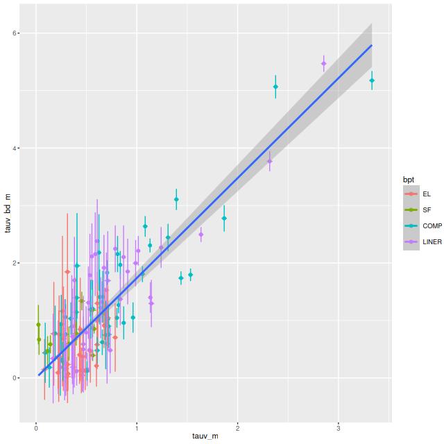
As a bit of an aside, my standard postprocessing includes estimates of dust attenuation of ionized gas using the Balmer decrement method with an assumed intrinsic ratio of Hα/Hβ = 2.86. Keeping only spectra with 3σ detections in both I get the following relation between gas and stellar attenuation. The slope of the straight line from a simple linear regression is 1.74 ± 0.06 (1 σ), which is consistent with their results (section 4.3) and, I think, other literature sources.

NGC 2623 (MaNGA plateifu 9507-12704) – Ionized gas τ_V vs. stellar τ_V for regions with detections in both Hα and Hβ

For reasons that escape me in paper (a) they chose to examine stellar population ages in 3 broad ranges: young (t ≤ 140 Myr), intermediate (140 Myr < t ≤ 1.4 Gyr), and old (t > 1.4 Gyr). I have a routine to calculate mass fractions in arbitrary age ranges, so I reproduce their figure 8:

NGC 2623 (MaNGA plateifu 9507-12704) – radial distribution of mass fraction in “young”, “intermediate,” and “old” populations

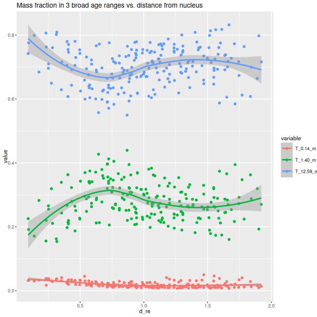
In contrast to their result there is no location where there is as much mass in “intermediate” age stars as “old” ones. However, and in agreement with them, if the SFR were constant over cosmic history there should only be about 10-11% of the total mass in young and intermediate age stars, suggesting an enhancement in SFR of a factor of ~2-3 over the past ~Gyr.

I calculated the total (IFU wide) star formation rate by summing over all individual models. The histograms below are for 100 and 10 Myr time spans: the estimated SFR has actually increased, from ≈ 10.4 M_☉/yr to 13 M_☉/yr in the last 10 Myr, with nominal uncertainties of ±0.5. This is entirely driven by a recent increase in the near-nuclear SFR.

NGC 2623 (MaNGA plateifu 9507-12704) – model total star formation rate on 100 and 10 Myr time intervals

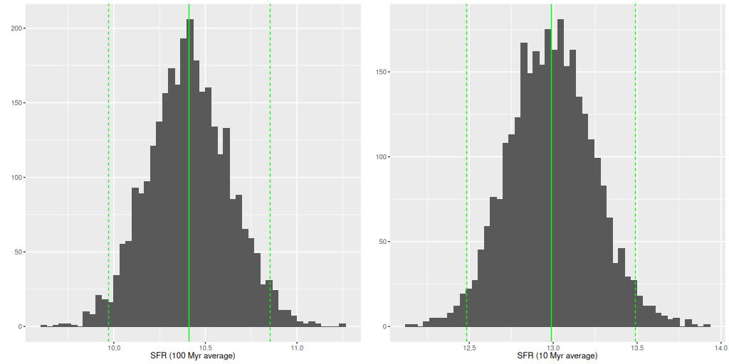
SFR estimates based on infrared data tend, understandably, to be higher — the literature sources I noted at the top gave estimates of 40-70 M_☉/yr. Cortijo-Ferrero give estimates of ~8-12 M_☉/yr depending on time span considered.

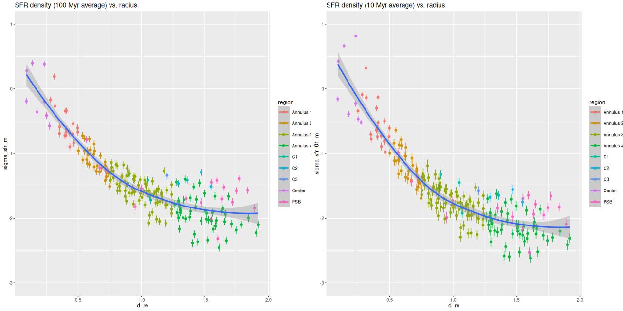
Paper (b) chose a different set of age ranges to focus on: 30, 300, and 1000 Myr, although they only discussed 300 Myr averaged star formation briefly. Instead of trying to reproduce their results for those SF timescales I’ll just show SFR density vs. radius for the 100 and 10 Myr lookback times that I’ve examined in this post. These can be compared to their figures 5 and 6. My 10 Myr plot for SFR density² looks similar to their 30 Myr except the peak values in the center are higher. In my models this is because the center has just turned on in the last <10 Myr.

NGC 2623 (MaNGA plateifu 9507-12704) – SFR density vs. radius/half light radius, 100 and 10 Myr time intervals

My sSFR plots don’t resemble theirs (figure 6) very closely. Both have a negative gradient within 1 half light radius while theirs have very shallow gradients. The steeper gradient in the 10 Myr plot is due to the recent central starburst and the slow decline of star formation outside the central few kpc.

NGC 2623 (MaNGA plateifu 9507-12704) –
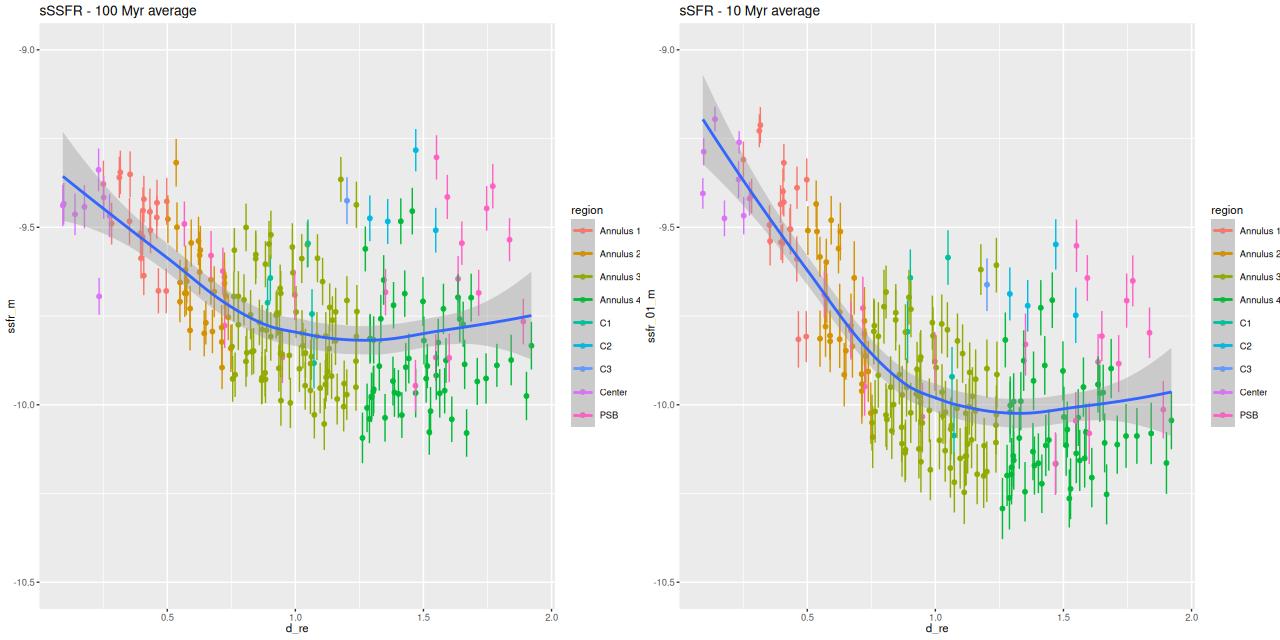
Specific star formation rate vs. radius in 100 and 10 Myr time interval. Units are yr^-1, logarithmically scaled.

Looking back at the SFH plots by region, there appear to be 3 epochs of accelerated star formation. The oldest begins at ~1 Gyr, the second at ~300 Myr, and finally there is a central starburst with age ≲10 Myr. Privon’s merger simulation, which is the only source for this system, places the first pericenter passage at ~220 Myr lookback time Without knowing what level of accuracy to expect from this kind of simulation this appears to be excellent agreement, so we can confidently associate the “pie wedge” with this event, as well as the enhancement in SFR at about the same age in the very center.

What’s more puzzling is the apparent increase in SFR long before the final stages of the merger. In most recent high resolution simulations that I’ve seen SFR increases above baseline only shortly before first pericenter passage (e.g. Renaud et al. 2014).

Slightly puzzling also is that if coalescence occurred ~85 Myr ago as in Privon’s simulation there is no trace of its effect in my models. The current central starburst must have been delayed considerably compared to the predicted almost immediate starburst in recent simulations.

This is one of about 10% of candidate PSBs in the Leung et al. sample that was rejected for further analysis based on fitting issues. Oddly, this was classified as a Central PSB, which is clearly wrong (and which a cursory literature search would confirm). Their fitting issues may have arisen from their strategy of binning all spectra meeting their PSB criteria into a single one. This can’t work when physical conditions, particularly dust attenuation, vary rapidly.

I have recently, after several months of leisurely computing, completed model runs for all 91 data sets in this sample. A detailed analysis is some ways off. I need to go through each model run — some had very poor fits, possible calibration errors, or low S/N data.

2026-01-14

NGC 2623 – part 2

I’m going to continue my discussion of the models for the MaNGA observation of NGC 2623 (aka Arp 243, etc.) in MaNGA plateifu 9507-12704 (mangaid 1-605367). First I’ll look at emission lines and line ratios. I don’t have any fresh insights to offer, but it’s useful for me at least to compare to earlier IFU based studies by Lipari et al. (2004) and Cortijo-Ferrero et al. (2017).

Next I’ll turn to stellar populations and star formation histories. This will prove to be quite interesting: there are several distinct regions in different evolutionary states. That will be in my next post.

Emission line properties

For an overview the plot below maps the Hα flux density¹ uncorrected for attenuation. The values are logarithmically scaled. The brightest region by some margin is just NE of the nucleus, with a secondary peak a short distance to the east. The three brighter areas to the south of the nucleus are H II regions.

The right hand panel shows BPT classifications from the [O III] 5007/Hβ vs [N II] 6584/Hα diagnostic following Kauffmann (2003), augmented with a weak line class for spectra without firm detections in one or more of those lines or [O II] 3727-3729 (labelled “EL” in the graph), and another (“NO EM”) for spectra with no firm detections at all. Just over half of the spectra have too weak lines to classify, while 40% fall in the LINER or “composite” bins mostly in a connected region surrounding the nucleus. The three regions in the south have unambiguously starforming BPT classifications.

NGC 2623 (MaNGA plateifu 9507-12704) – (L) Hα flux density. (R) BPT classification from [O III]/Hβ vs [N II]/Hα per Kauffmann 2003

The shape and relative values of the Hα flux near the nucleus agree very well with a higher resolution map published by Cortijo-Ferrero:

Screenshot of Hα flux density from Cortijo-Ferrero et al. 2017

Taking a closer look I plotted line ratios for the 3 BPT diagnostics that are commonly used with SDSS data, namely [O III] 5007/Hβ vs. [N II] 6584/Hα, {S III] 6717+6730/Hα, and [O II] 6300/Hα. Only points with 3σ detections in the relevant lines are plotted. Lines marking the boundaries between star forming and something else are from Kewley et al. (2006) and Kauffmann (2003). Note that in all 3 plots the regions with star forming line ratios stay on the star forming side of the boundaries, as do the areas with LINER like ratios. The “composite” regions on the other hand are in the star forming side of the boundary in the [SII/Hα plot while many shift into the LINER region in [O I]/Hα.

NGC 2623 (MaNGA plateifu 9507-12704) – BPT diagnositcs for commonly used emission line ratios: (L) [N II]/Hα, (C) [S ii]/Hα , (R) [O I 6300]/Hα. Lines are SF/something else boundaries from Kauffmann 2003 and Kewley 2006. Only spectra with 3σ detections in the relevant lines are plotted.

There’s a fairly general consensus on the likely ionization sources. X ray observations demonstrate the existence of a heavily obscured low luminosity AGN (e.g. Yamada et al. 2021 and many others) along with a nuclear starburst. Just outside the nucleus shock excitation was proposed as the main ionizing source already by Lipari, and confirmed by Cortijo-Ferrero’s CALIFA observations, although they also emphasize the possible role of recent star formation.

Alatalo et al. (2016) commented that “[O I]/Hα is a particularly good tracer of shock excitation,” citing Rich et al. (2010) and another source. The latter is particularly interesting because they performed a detailed IFU based analysis of a galaxy (NGC 839) that, while not being involved in a merger, shows similar properties of moderately high velocity outflow probably driven by a nuclear starburst with extensive regions of post-starburst spectra. Their BPT plots look remarkably similar to mine, with most spectra in the “composite” region in the [N II]/Hα plot shifting into the LINER region in [O I]/Hα.

Maps of the line ratios are shown below: again only regions with 3σ detections in the relevant lines are shown, which considerably limits the spatial coverage of [O III]/Hβ and [O I]/Hα. A few points to note: the peak value of [O III]/Hβ is just NE of the nucleus and likely near the source driving the outflow. All of the line ratios generally increase away from the nucleus to the NW and NE. To the south the three H II regions are prominent.

NGC 2623 (MaNGA plateifu 9507-12704) – Maps of emission line ratios. (TL) [O III 5007]/Hβ (TR) [N II 6584]/Hα (BL) [S II}/Hα (BR) [O I 6300]/Hα. Only spectra with 3σ detections in the relevant lines are shown.

The main result of this analysis is it validates my approach of modeling emission line and stellar contributions simultaneously. This is uncommon but not unheard of in the spectral fitting industry². Since some form of stellar template is needed to get unbiased estimates of emission line properties, from my point of view it makes sense to model both at once. My results for this galaxy agree very well with the two earlier major studies.

I’m going to hit publish now and continue with stellar populations in my next post. I may actually have something new to say about them.

2026-01-082026-01-09

NGC 2623

I’ve been making my way through Leung’s PSB sample and noticed this exceptionally interesting “CPSB” sample member, which oddly enough they chose not to include in their analysis. This is NGC 2623, a rather famous merging galaxy pair that was one of Toomre‘s exemplars of a late stage merger. This is a well studied system, with over 500 references listed in NED and observations apparently in every electromagnetic frequency range for which telescopes exist (nothing from JWST yet though).

MaNGA targeted it with one of their largest IFUs, which covers most of the visible light (at the depth of SDSS imaging) of the merger remnant, but very little of the tidal tails. There’s also a CALIFA IFU dataset with a larger spatial footprint but lower spectral resolution. I haven’t looked at that in detail yet except to estimate the relative velocity field..

As usual I work with RSS spectra stacked and binned to a target S/N. For this final post starburst project I’m trying to set a higher S/N threshold. In this case I ended up with 214 spectra with S/N per pixel ranging from 8.5 to 42.5.

MaNGA plateifu 9507-12704, mangaid 1-605367

Kinematics

I’ll first discuss the stellar and gas kinematics, since calculating redshift offsets is the first thing I do after loading data and binning to a target S/N. I use a straightforward template matching procedure using as templates a set of 15 eigenspectra that I computed some years ago using an algorithm published by Blanton and Roweis (2007) and a fairly large sample of SDSS galaxy spectra. The first 5 are shown below. The first two look like real spectra of a passively evolving ETG and a star forming galaxy respectively. The rest represent departures from these archetypes. I did not mask emission lines, so both absorption and emission lines are present, often with the opposite of expected signs.

First 5 eigenspectra used as templates for calculating redshift offsets

Here is the computed velocity field (converted from redshift offsets from the published system redshift of z=0.01818). As I’ve said before and is obviously the case from the plot above the template fitting procedure gives a blended velocity estimate that in any given spectrum might be dominated by emission, absorption, or a combination. In this case it turns out that emission lines dominate in the IFU center, with the outer parts dominated by stellar motion.

NGC 2623 (MaNGA plateifu 9507-12704)
velocity field from template fit

I often check Marvin to compare MaNGA data analysis pipeline measurements to mine. Sometimes visual comparisons are hampered by unfortunate choices of color palettes by the Marvin team. That’s especially the case for velocities where they use shades of red, white, and blue to represent positive, ~ 0, and negative velocities. It was apparent though that the stars and gas are kinematically decoupled at least in the center.

To investigate further I decided to dust off my old code for non-parametric line of sight velocity distribution modeling¹, made some small modifications, and ran on the same 214 binned spectra. The results for the mean velocity offsets from the system redshift are shown below for stars (L) and gas (R). For easier comparison to Marvin I interpolated the model outputs to 0.5″ x 0.5″ pixels.

Even though people who claim to know generally disapprove of the use of rainbows in graphics I like to use them for velocity maps. In this case though using a more perceptually uniform palette (viridis with 256 levels) reveals some interesting details that aren’t as evident with a rainbow palette.

NGC 2623 (MaNGA plateifu 9507-12704) Estimated stellar and ionized gas velocity distributions.

I also downloaded the maps from Skyserver that are displayed in Marvin. Below are the stellar and Hα velocity plots². I haven’t tried a detailed quantitative comparison because it’s not easy to properly register the maps, but it’s evident that these are very similar.

NGC 2623 (MaNGA plateifu 9507-12704) Estimated stellar and ionized gas velocity distributions from MaNGA DAP.

The velocity maps have several interesting features. First, the ionized gas is rapidly rotating within the inner ~2 kpc, but there’s no apparent organized rotation farther out. Zooming in on the center the rotation axis appears to be offset to the east of the IFU center (marked), which is exactly at the position of the nucleus, by ≈ 1.6″ (800 pc) if the unlabelled 75 km/sec contour line is taken as the axis of rotation. In a very thorough analysis of IFU data that preceded MaNGA by more than a decade Lipari et al. (2004) also noted a displacement of the kinematic center of 1.1″ to the east of the nucleus — in good agreement with my estimate given the limited resolution of MaNGA data. There also appears to be good qualitative agreement on gas velocities in the area with overlapping observations, which is roughly the zoomed in region below (see their figure 8a). NGC 2623 was also observed in the CALIFA survey, and its kinematics are discussed in Barrera-Ballesteros et al. (2015). Their velocity fields appear broadly similar, but visual comparison is hampered by the small size of their figures.

Outside the nuclear region gas and stellar velocities are more nearly equal although with some scatter that may simply be due to measurement errors.

A minor point that’s maybe worth noting is the overall mean velocity in both the stellar and gas measurements is ≈70 km/sec, which suggests the system redshift of z = 0.01818 adopted by MaNGA is low by ≈2×10^-4, or z = 0.01842 (cz = 5522 km/sec). This is close to the fiducial heliocentric redshift of 0.01851 adopted by NED and well within the range of values listed there.

Two features I find really interesting that are especially prominent in the stellar velocity map are a pair of long, irregular, but mostly connected arcs that stretch across the full width of the IFU. One arc is relatively redshifted, exiting (entering?) the IFU at the position of the small portion of the SW tidal tail that’s within the footprint, appears to cross the other arc, then stretches to the south and east of the nuclear region, terminating to the north approximately where the northern tidal tail enters the IFU footprint. The other, relatively blue shifted arc starts in the south in the area of the blue, wedge shaped region (which I will discuss much more later), curves around to the west of the nuclear region, and appears to terminate somewhere in the NW region of the IFU.

To date there is only one N-body simulation of the NGC 2623 merger, by Privon et al. (2013). In their model the blue wedge in the south is material from the progenitor that formed the northern tidal tail, has passed through the main body and is now falling back in. In their simulations there are regions even in the main body of the merger remnant where the progenitors aren’t well mixed. I’m wondering if these apparently connected regions with systematic velocity offsets might reflect that lack of complete mixing, with the blue shifted regions falling into the galaxy from behind and the redshifted falling from above.

One final plot for now: the average emission line velocity dispersion. These are “raw” values uncorrected for spectral resolution. The relatively high values to the NE of the nucleus might be associated with the outflow discovered by Lipari et al. The low values well south of the nucleus are from H II regions.

NGC 2623 (MaNGA plateifu 9507-12704) mean Ionized gas velocity dispersion

This post turned out longer and took longer to write than I expected, so I will break it up into two or perhaps more. Next time I’ll look at some other physical properties and perhaps model star formation histories.

Update

Barrera-Ballesteros found regular stellar rotation out to the maximum radius of 6″ (2.2 kpc) that they had usable data. Both they and Lipari found a sinusoidal rotation curve for the ionized gas. I was skeptical of the claimed large scale stellar rotation since visual inspection of the velocity maps didn’t show an obvious velocity gradient in any direction. But, I decided to take a closer look anyway. Since the kinematic position angle for both is close enough to 90^o I just plotted velocities for bins within ±2″ of the horizontal axis. The results are plotted separately for stars (L) and gas (R). The curved lines with “confidence bands” are loess fits to the plotted data and should absolutely not be taken seriously as a model of the rotation curves. It’s notable though that if’s fairly symmetrical for the stellar velocities and if the true system velocity is 70 km/sec larger than adopted by MaNGA its kinematic center is right at the IFU center. The ionized gas kinematic center is clearly seen as offset to the east, as noted above.

NGC 2623 (MaNGA plateifu 9507-12704) – Stellar and gas velocities within 2″ of the X axis

2025-12-22

A small course change

After a bit of a break caused by spiking electricity bills and travel I’ve resumed the program I discussed in my last post, but with a change in the sample I’m drawing from. While traveling a few months back I noticed a (now published) preprint on arxiv titled “The diverse quenching pathways of post-starburst galaxies in SDSS-IV MaNGA,” by Leung et al. (2025). This was a companion to Leung et al. (2024) and evidently part of the first author’s PhD research. These two papers studied “ring” and “central” post starburst galaxies (RPSB and CPSB), a morphological dichotomy originally noted in Chen et al. (2019), and studied further with data from the final MaNGA data release by Cheng et al. (2024)¹. A third category of “irregular” psbs hasn’t received much attention, probably because the majority of those are likely to just be spiral galaxies observed with enough resolution to sample interarm regions.

The two papers by Leung et al. were of interest for a couple of reasons. First, they published catalogs of their sample as supplemental data to the journal papers, and the sample was reasonably sized for my resources: a total of 91, with 50 cpsbs and 41 rpsbs. This is comparable size to the 103 SDSS selected K+A candidates that I started to run models for, and there is some overlap in objects: 17 of my sample are in the cpsb sample, and 3 in the rpsbs. In addition 6 out of 8 of Melnick and dePropris’ SDSS based compilation are in the cpsbs, and 9 are drawn from the PSB ancillary program sample.

Another point of interest was they published star formation history models for their entire sample (minus a few that they chose not study further). Their methods are quite different from mine and I have no intention of trying to reproduce their work in any detail, but it will be of some interest to see if burst timescales and strength are at all comparable.

Modeling the chemical evolution of the stars through the bursts was an important part of these papers. Although I was and remain skeptical of the ability of my models to say much about stellar chemical evolution I have added metallicity tracking to my data analysis pipeline. I’m making this as simple as possible: for each age bin and each sample draw I calculate the mass weighted metallicity from the nominal Z values listed in the library. The present day stellar metallicity is similarly calculated as the remnant mass weighted metallicity summed over all SSP model contributors. As I’ve said before my models have nonzero contributions from all age and metallicity bins in the inputs, which can’t really make sense in any realistic chemical evolution scenario, so if they have any use at all it’s likely to be in the mean.

As of the date of posting I’ve run models for about 3/4 of the sample using my standard Stan model and the “medium” size SSP model library. I haven’t attempted any detailed analysis of results yet, but I do look at some graphs as model runs complete. I have noticed a few fairly consistent themes which I will illustrate with a single unremarkable galaxy from the cpsb sample, with plateifu 8655-1902 (mangaid 1-29809):

SDSS “finder chart” image of SDSS J235352.51-000555.3 — MaNGA plareifu 8655-1902 (mangaid 1-29809)

I’m trying to increase the minimum nominal signal to noise to average around 8 per pixel, although that isn’t always feasible. In this case the stacked RSS file binned to 15 spectra with a SNR range of 8.2-22.9. Here are the model star formation rate, mass growth, and metallicity histories for all 15 bins arranged by distance to the IFU center. The SFR scales are allowed to vary while the other two have fixed vertical scales. Lookback times are scaled logarithmically.

SDSS J235352.51-000555.3 — MaNGA plareifu 8655-1902 (mangaid 1-29809)

Modeled star formation histories, mass growth histories, stellar metallicity histories — binned spectra ordered by distance from center

One thing I’m noticing in the sample (both cpsbs and rpsbs) is a distinct tendency for bursts, where they appear in a model, to peak at right around 1 Gyr. Is there something in the sample selection criteria that favors a rather narrow range of burst ages, or is it some peculiarity of this SSP model library? It could be either. Taking the models literally this galaxy did indeed have a centrally concentrated but widespread burst, with some outer regions heving slightly enhanced star formation with quenching at about the same time as the center.

As the third set of graphs show the models don’t even “claim” to constrain stellar metallicity to any great degree. This version of the library has only 3 metallicity bins: Z = {0.011, 0.02, 0.063}, and the credible interval bands cover essentially the entire range of inputs. Somewhat surprisingly though there do appear to be systematic changes around the time of the burst. In this case the center shows a small decline in metallicity while most of the outer regions have a sharp increase that decays to a mean value a little larger than the pre–burst metallicity. I can’t quite make sense of this, but it does actually agee with Leung’s results.

Here is the (posterior predictive) fit of the model to the central fiber spectrum:

MaNGA plateifu 8655-1902 (mangaid 1-29809) — central fiber spectrum, PP model fit, and residuals

There aren’t any long stretches with systematic departures from the observations, except for a slight upturn in the residuals at the reddest wavelengths. This seems to be relatively common: the continuum sometimes turns sharply upward at the reddest wavelengths — this gets flagged as a “blowtorch” in the MaNGA data reduction pipeline and along with night sky lines make the reddest 1000Å or so useless for analysis. I may decide to truncate the SSP model spectra at a slightly shorter wavelength, but for now I will continue the analysis with the current library version.

I will put off further analysis until I’ve finished model runs. Should be another week or two.

2025-08-26

Back to real data; brief update

This will be short. I’ve provisionally decided to proceed with the Progeny based SSP model libraries I’ve discussed over the last several posts. I’ve picked two versions for model runs: a “small” one with 5 metallicity bins and 42 age bins from log(T) = 6 to 10.1 in 0.1 dex intervals, and a “medium” sized one with just 3 metallicities (log(Z/Z☉) = {-0.25, 0, +0.5}) and 74 age bins with log(T) = 6.0, 6.5 and 6.55, … , 10.1 in 0.05 dex intervals. These all use the MIST isochrones, Kroupa IMF, and the recommended stellar ingredients from the first Progeny paper. As discussed in a previous post the wavelength interval is limited to 3300 – 9000Å because of the prevalence of terrestrial night sky lines and calibration issues in the near IR portion of MaNGA spectra.

I’ve decided to take one more, maybe final, look at a sample of SDSS selected galaxies in MaNGA. I remembered recently that I’ve made several attempts to select post-starburst samples with various queries of SDSS databases. One I did some time ago had nearly 5800 hits in DR8, with 104 cross matches in MaNGA. Part of the query is pasted below:

select into mydb.mylargerka
  s.ra,
  s.dec,
  s.plate,
  s.mjd,
  s.fiberid,
  s.z,
  s.zErr,
  from specObj s
  left outer join galSpecline as g on s.specObjid = g.specObjid
  left outer join galSpecIndx as gi on s.specObjid = gi.specObjid
  left outer join galSpecExtra as ge on s.specObjid = ge.specObjid
where
  (g.oii_3729_eqw > -5 and g.oii_3729_eqw_err > 0) and
  (gi.lick_hd_a_sub > 4 and gi.lick_hd_a_sub_err > 0) and
  s.z >= .02 and
  (s.snMedian > 10) and
  (s.zWarning = 0 or s.zWarning = 16)
  order by
  s.plate, s.mjd, s.fiberid

So basically this is just a standard sort of post-starburst selection with relaxed limits on both Balmer absorption and emission line strength. The line index data were from the MPA/JHU pipeline, which was last run on DR8.

I had run models for about 1/4 of the 104 galaxy sample when a heat wave arrived, and I decided for the sake of our electric bills not to continue intensive computing 24/7. Temperatures are currently below normal, so I may be able to resume soon. About all I can say so far is the sample contains a mix of known PSBs and false positives — which are mostly ordinary star forming galaxies.

2025-06-292025-07-04

Brief simulations update, and some related literature

A few brief comments about the simulations, of which I’ve done a few more but will probably bring to an end. First, here is a plot I mentioned but didn’t display last time of the bias in stellar mass estimate against the lookback time to the burst. Points are color coded by burst strength.

Bias is stellar mass estimate vs. lookback time to burst (simulations)

There appears to be a weak trend with burst age up to about 1 Gyr, but at all burst ages and strengths there are biases on both sides of zero. It isn’t clear to me what, if anything else, is driving biases in either direction. The one thing I can say for sure is that the models are overconfident in their ability to estimate the stellar mass since the typical 1σ error bar is under 0.02 dex while the scatter is around ±0.1 dex. I actually think 25% uncertainty in stellar mass estimates is optimistic.

I remembered a short while ago that “outshining” is the term of art in the industry for the situation in which light from recent star formation overwhelms that of the older population. This seems to be a fairly major concern in the literature. A full text search of ADS found 722 instances of its use in the astronomical literature with an explosion of usage after 2006. A quick scan of titles suggests perhaps half of the papers are about SFH modeling. Of course the word is often used in other contexts.

As a slightly more stringent test for outshining I ran one more simulation with a more recent and stronger starburst (t_b=0.25 Gyr, f_b = 1) than the earlier simulations. Even though the light of the burst population dominates the old base population the latter does have some effect of the combined spectrum (in red below, and offset vertically for clarity): it is redder and the line strengths are altered somewhat relative to the burst population.

Synthetic spectra – strong recent starburst. Fluxes are logarithmically scaled. Total flux (red) is vertically offset.

The model actually captures both the ancient and recent star formation history rather well. The mass growth marginal confidence band at old ages covers the input right up to the beginning of the burst build up, and the post-burst SFR is modeled accurately. The total mass in the model slightly exceeds the input: log(M_*) = 4.88±0.02 model, 4.84 input. The model specific star formation rate is nearly identical: -9.33±0.08 model, -9.36 input.

Shortly after starting these simulations I noticed a paper by Suess et al. (2022) describing simulations with a similar objective of testing the ability of a code named PROSPECTOR to recover star formation histories of post-starburst galaxies in the ideal case of inputs matched to the model, i.e. the inputs are used to generate the mock data and then to fit it. I’m not going to say a lot about either the code or paper. IIRC the first published description of the code (Leja et al. 2017) claimed it to be the first to model non-parametric star formation histories in a fully Bayesian framework. As far as I know this is true in the published literature but they only could use a few very broad time bins; the version used in Suess uses 9. I was already using the full time resolution of my adopted SSP model libraries by then.

The 2022 paper only shows a single, no doubt cherry picked example of a fit to mock data. Like mine their model star formation histories fail to cover the inputs for some age ranges. On the other hand their fits to a mock spectrum appear to be rather poor with large systematic errors. In every model run of mine residuals look very much like 0 mean Gaussian white noise with the expected deviance. They appear to show a similar range of deviations from input stellar masses with no significant error in the mean. Another striking similarity is they find a definite floor to late time star formation rates. As I’ve noted many times my models will always include some contribution from very young populations and there seems to be a floor around 10^-11.5 /yr in specific star formation rate.

A much more recent paper by the same group (Wang et al. 2025) looked at simulated data from quite different systems, namely ones with bursty star formation on short time scales. Their work was motivated by yet more simulations of galaxy formation in the early universe. I’m again not going to comment much on this paper except to notice that they concluded that “given the correct SFH model, it is indeed possible to infer the SFH by performing SED fitting.” In other words they had to fine tune their prior to get to the right posterior. I’m sure it’s not as tautological as that sentence appears. Anyway, this motivated me to take a brief look at a few multiple burst simulations. The one shown below has two very sharply peaked ones with roughly the same peak SFR but more total mass in the older one. The model has spread out star formation over the entire interval between the input bursts with a slower rise and decay. Once again the maximum likelihood fit obtained with non-negative least squares captures the timing and relative magnitude of the bursts rather well.

Recall that my stellar contribution estimates are parametrized as an N-simplex with an implicit Dirichlet prior with concentration parameter α = 1, which is uniform on the simplex. In principle adopting an explicit prior with a concentration parameter < 1 should encourage a more bursty star formation history without favoring any particular ages, and it did (this run used α = 0.25):

Simulation – 2 short starbursts, modified prior

Here are histograms of a few summary quantities I track: the present day stellar mass, specific star formation rate (100 Myr average), and the summed log-likelihood of the fits to the spectra. Both runs underestimated the sSSFR because the recent burst was more spread out in the models.

Two burst simulation: comparing two priors on stellar contributions for sampled stellar mass, SSFR, and log-likelihood of fits

Finally, I did a few runs with two other libraries: EMILES, which has been my base SSP model library for some time, and BPASS with single star evolution and an upper mass limit of 100 M_☉. The parameters I used for the star formation history resulted in a gentle late time revival rather than a burst. Both model runs had late time bursts, although the mass added was negligible. The EMILES run has the characteristic jumps at ages where the age intervals change. Although it’s small the BPASS run has the jump at 1.6 Gyr that I noted previously.

Simulation with C3K input and EMILES as test library

As with real data the EMILES models have some systematic errors around the trough around 7000-7300Å, and also in the blue near the Balmer break.

The BPASS models fit the data surprisingly well, despite using completely different sources for stellar atmospheres.

Comparison PP fit with C3K as test library:

The table below summarizes a couple of the quantities I track. The Progeny C3K models that were used to create the inputs recovers them flawlessly. The other two recover the mass (BPASS is low by more than its nominal uncertainty), but are biased on the high side in late time star formation rate estimates.

	Stellar mass	sSFR
input	4.78	-9.91
Progeny C3K	4.78 (0.017)	-9.90 (0.054)
EMILES	4.82 (0.012)	-9.62 (0.028)
BPASS	4.67 (0.03)	-9.73 (0.049)

I’m going to get back to real data now using the Progeny generated libraries. The simulations were a useful exercise if for no other reason than to show that timing faded starbursts can’t be done very accurately, at least with full spectrum fitting at visual wavelengths. I did get some ideas for small code improvements, and the idea of stacking star formation rate and mass growth histories seems like a useful visualization tool.

2025-04-05

Back to simulating star formation histories

I’ve decided to take a break from real galaxy data and run some simulations of synthetic galaxy spectra. The main motivation was to help make an informed decision about which subset of the ProGeny based SSP libraries to use: the ones based on the MIST isochrones have ages uniformly logarithmically spaced at 0.05 dex intervals and 15 metallicity bins. Most of the latter are considerably sub-solar and aren’t likely to be major contributors to the light of nearby massive galaxies. For possibly metal poor dwarf galaxies it’s always possible to pick a metal poor subset — I have a subset of EMILES that I’ve used for that purpose for some time. More important to me is the choice of age bins. As I mentioned in the last post I did model runs with both 42 (0.1 dex age intervals) and 83 ages, with SSP models younger than log(T) = 6 and older than the currently accepted age of the universe excluded. Since execution time of a Stan model is roughly proportional to the number of parameters and these models are rather time consuming I’d like to know if the coarser age spacing has sufficient resolution. I will show below why it’s correct to exclude the very youngest populations.

Other reasons to do these kinds of exercises are to test the accuracy of retrieval of key quantities in idealized conditions where model assumptions are met by the inputs, to compare different model libraries, or to compare different modeling codes (something I don’t plan to do at present). Performing simulations is de rigueur in the SFH modeling industry and there are many examples in the literature, both as appendices and standalone papers — to name one the second of the two ProGeny papers I linked last time falls in this category. I’ve even done some limited simulations as far back as 2018, but the only case I wrote about was a very simple one.

This time I’ve decided to be more systematic and at least slightly more realistic. Since I remain interested in post-starburst galaxies I am creating simulations with two components: a base population that begins forming stars at the beginning of the universe, which I take to be a lookback time of \(10^{10.125}\) yr. = \(13.36\) Gyr. The second component is a “burst” population that commences star formation at a lookback time of \(\mathsf{t}_b\) with a relative strength of \(\mathsf{f}_b\). The base population has solar metallicity (Z = 0.02) while the burst is slightly subsolar (log(Z/Z_☉) = -0.25). This obviously isn’t meant to represent a realistic model for chemical evolution — the purpose again is to test the ability to recover the input stellar metallicities in idealized circumstances. In keeping with my usual attitude of treating this as an afterthought I haven’t gotten around to exploring this issue yet.

Both the base and burst populations have time varying star formation rates proportional to Gamma probability distributions. The Gamma distribution is a two parameter family of univariate functions that can have a fairly wide variety of shapes, all of which have a single mode at \(t \ge 0\) followed by a monotonic decline asymptotically approaching 0. See the table below for the most salient properties. I don’t know of any real astrophysical justification¹ for this choice but it’s notable that it includes two of the most popular parametric forms for modeling star formation histories: exponentially declining (\(\alpha = 1\)), and what’s generally called the “delayed-\(\tau\)” model (\(\alpha =2\)) in the literature. Note that using a probability distribution has nothing to do with probability per se, but a probability density has two useful properties: it’s non-negative on its support and has a finite integral (equal to one when properly normalized).

Property	Value
Parameters	shape \(\alpha \ge 0\) scale \(\theta > 0\)
Density function	\(f(t) = \frac{1}{\Gamma(\alpha)\theta^\alpha} t^{(\alpha-1)}\mathsf{e}^{-t/\theta}~~t \ge 0\)
Mean	\(\alpha\theta\)
Mode	\((\alpha -1)\theta~~\alpha\ge1\) \(0~~~~\alpha \le 1\)
Variance	\(\alpha \theta^2\)

Source: Wikipedia

Given shape and scale parameters the mass in each time bin is proportional to the difference in the cumulative gamma distribution at the beginning and end of each interval. The star formation history for each component is just the mass formed in all age bins, with the burst component multiplied by the burst strength. These are scaled to sum to 1, and the spectra are straightforwardly calculated as matrix products of the input SSP model fluxes with the mass histories. The “flux” values are multiplied by 10⁵ for the sole purpose of making them approximately unit scaled. This has the effect of making the total mass born in the simulated “galaxy” equal to 10⁵ M_☉. The fluxes are interpolated to the same logarithmic wavelength grid used by SDSS, convolved with a gaussian to simulate stellar velocity dispersion, then truncated to the wavelength range (3621 Å, 9000 Å). The velocity dispersion is a settable parameter, but so far I have only used 140 km/sec. The base and burst spectra, which were calculated separately for visualization purposes are added, then multiplied by Calzetti attenuation with a user selected optical depth, then finally perturbed with Gaussian random noise. The flux variances are Poisson-like, that is they are proportional to the “counts” in each wavelength bin and scaled to a target average signal to noise. Again this is a settable parameter, but so far I have used a target SNR of 40, which is fairly typical for a fiber spectrum near the center of the IFU of a bright MaNGA galaxy. So far at least I do not add emission lines, but they are allowed in the models.

The subsequent modeling workflow is essentially the same as I use with real data, with some very minor tweaks reflecting the fact that the flux values are arbitrarily scaled. The Stan code is exactly the same as my current working version. Model runs use the same number of warmup and sampling iterations as my real data runs (250 and 750 respectively with 4 independent chains). Post processing is also essentially the same. I extract the posterior predictive fits to the spectra, the model star formation histories, the optical depth of attenuation and the reddening curve slope parameter. I compute the present day stellar mass, the 100 Myr averaged star formation rates, and specific SFR. The stellar mass and SFR are arbitrarily scaled but would scale by the same factor if these were real data from a distant galaxy, so the SSFR would be the same.I also track a few observables: the 4000 Å break index D_n(4000) and Hδ_A.

This time I am exploring a wider range of star formation histories than my previous effort, which only examined a case or two with instantaneous bursts. With seven parameters (plus two more that I’ve held constant so far) it isn’t really practical to do a comprehensive grid of models, so for the most part I have randomly selected parameter values in the ranges shown below. At the time of writing I’ve run a few more than a hundred models. Most of these use the “small” version of the ProGeny C3K base SSP models as the test library, with a few using the input library as the test. I’ve also done a few with the “large” version (see the previous post for details of the ingredients). I plan to do some simulations with the other model libraries I’ve used, especially EMILES, but that’s somewhat of a different project. For now I’m examining the accuracy of outputs for the idealized case where the inputs satisfy the assumptions of the model.

\( \alpha_0 \in [1, 2] \)

\(\theta_0 \in [2, 6] \)

\(\mathsf{t}_b \in [0.5, 2]\)

\(\mathsf{f}_b \in [0.1, 0.75]\)

\( \alpha_b \in [1, 2] \)

\( \theta_b \in [0.01, 0.25] \)

\( \tau_V \in [0.0, 0.5] \)

Here is a cherry-picked example of a fairly strong and recent burst, using the small C3K based library as the test. First is the “observed” spectrum and the replicated values from the posterior (top pane), and the posterior residuals (bottom pane). The residuals look very much like — and pass standard statistical tests for — Gaussian white noise. This is rather different than I usually see with real data, of which a number of examples can be found by scrolling down through previous posts, where there are often large regions of spectra that are systematically misfit. This reflects the fact that all model assumptions are met by the data by construction, so fitting the data is expected.

Simulated spectrum and “posterior predictive” fit and residuals.

The model star formation history from the same simulated data contains some surprises, and these turn out to be fairly generic features of most model runs. This is a bit of a new graphical display for me. I’ve put the star formation rate history above the mass growth history with the same age scale for each so I can get different views of the same sequence of events. The input model parameters are on a line in between. The blue lines are the input star (mass) formation history. The red line in the second plot is from the preliminary maximum likelihood fit. The black lines and grey ribbons are the marginal means and 95% confidence intervals. Reading from right to left there are several points to note:

The details of the pre-burst SFH are largely lost, although the total mass formed in the model is roughly the same.
The ramp up to the peak of the burst begins sooner and is more gradual than the input. Note that both the input SFR and mass growth are well outside the model confidence intervals in the ramp up period.
Most significantly in my mind at least, the peak of the burst is much later (more recent) in the model than the input. This turned out to be a fairly generic feature of these models.
In this run the post-peak decay is rather steeper on average than the input. In model runs with a rapid input decay the model will usually have a more gradual one.
The input and model SFR eventually converge and the late time model SFH agrees very well with the input, except
There’s an odd upturn in SFR at the very youngest ages (< 3 Myr). This happens to varying degrees in every simulation model run and in all the real data I’ve looked at. It turns out there’s a simple explanation for this. There is virtually no spectroscopic evolution in the relevant wavelength range in the first few Myr of a coeval population’s life. Since the spectra are indistinguishable there is no way to constrain the individual contributions without a more informative prior, and the models are correctly estimating the same marginal distributions for the youngest few populations. Since the time intervals get shorter with decreasing age this produces an apparent upturn in SFR.

Black line and grey ribbon: model results for SFH and MGH. Blue line: input. Red line: MGH from maximum likelihood fit.

ProGeny generated SSP model spectra — C3K base models – ages 1-10 Myr, solar metallicity

ProGeny generated SSP model spectra — C3K base models – ages 1-2 Myr, solar metallicity. Spectra are vertically offset.

There are two surprises in the simulations I’ve run so far. First is that, like the example above, the time of peak star formation in the model burst tends to be biased downwards (more recent) from the input. The bias gets larger in magnitude with increasing lookback time to burst onset and can be as large as several hundred Myr as seen below. The few outliers here were weak bursts with very large variations in the time of maximum SFR.

Bias in time of peak SFR vs. input burst onset time

The other surprise is that the 95% confidence bands of the model star formation histories, whether viewed as SFR or mass growth histories, fail to cover the inputs for at least some epochs around the time of the burst. In other words the models are saying that the actual input star formation histories are highly unlikely. Why is this?

It’s not, I think, because of any convergence failure. Stan is quite aggressive at flagging potential issues and there were virtually none in any of the model runs. I also don’t think it’s because the model runs were too short. I’ve occasionally gathered much larger samples with longer warmup times as well and except for exploring the tails of the distributions a little more thoroughly there is little change in marginal 95% confidence intervals.

Most of the model runs were done with the reduced size SSP library with just half of the available age bins (0.1 dex intervals). This doesn’t seem to have reduced the real effective age resolution, but in the small number of runs I did with the full set of ages the marginal contributions have larger confidence intervals, so this could increase the coverage.

I suspect though that the prior on the star formation history is having a larger effect than I would have suspected. The main clues here are the maximum likelihood fits. which often produce mass growth histories (the red lines in the plot above and the ones below the fold below) that are rather close to the input MGH, also falling outside the 95% model confidence bands for at least some epochs. In my current workflow the slightly perturbed maximum likelihood solution is used to initialize the Stan model. In most of the model runs the samples quickly move away from the initial values. While the fits to the data are good in all model runs the summed log-likelihood of the sample spectra is always less than the maximum likelihood solution, in the sample shown below by about 7%.

Log-likelihood of posterior samples and maximum likelihood solution for a simulated model run

Below the fold I’ve posted some more cherry picked examples of model star formation histories. A few general comments about them:

The late time star formation rate is generally well captured by the models.
The ancient (pre burst) star formation history is sometimes captured well with weak bursts. Particulary noteworthy is the second example below, which has a recent and weak burst with a gradual ramp up and decay. The entire star formation history is modeled accurately. In the literature there are sometimes references to “outshining” or a “dazzle” effect in (post)-starburst galaxies. This seems to be a real thing.
Early time bursts aren’t necessarily recognizable as such. In some cases the model just shows an extended period of star formation followed by more or less gradual quenching. I believe this is consistent with some claims in the literature, but I don’t care to look for the relevant papers right now.

I’ll conclude with a look at results for all simulation runs (so far) for some of the summary quantities I track. First, the present day stellar mass is on average unbiased but in individual runs there are errors as large as ±0.1 dex. The typical posterior uncertainties are only ~0.01 dex, so the models are consistently too optimistic. I’ve noted this in real data, which shows similar nominal uncertainties with moderately high S/N data.

Not shown here but I did notice a weak dependence on the input burst onset time or time of maximum SFR in the sense that recent bursts tend to underestimate the stellar mass. This is another possible manifestation of the “outshining” effect.

Error in model stellar mass vs. input stellar mass

The most dramatic bias is a tendency to overestimate the specific star formation rate when the input SSFR is low. This is also something I’ve seen in real data: as I’ve noted a time or two even the reddest and deadest of ellipticals seem to have a floor of about -11.5 for the estimated SSFR.

One thing I didn’t think about until finishing this analysis is that the contribution estimates tend to be skewed to the right when they’re near 0, so the median might be a better estimate of central tendency than the mean. That might make a (probably) small difference. I will look into this.

Error in model specific star formation rate vs. input SSFR

Finally, there’s a nearly linear relation between the error in the posterior estimate of the optical depth of attenuation and the input. Note also the stratification of the reddening slope parameter δ: at relatively high input optical depths the largest departures have the reddest attenuation curves. I think this behavior is directly related to the prior. Since I don’t think the attenuation is very well constrained by the data I use fairly informative priors on both the optical depth and slope parameter; both priors are truncated normals with a lower bound of 0 for τ_V and a range of (-0.5,1.2) for δ. This is an easy thing to test simply by changing the priors for these parameters.

Mean and standard deviation of model optical depth – input optical depth vs. input optical depth

I am not quite finished with these simulations. I want to expand the range of input parameters a little bit, and I need to look a little more carefully at subsets of the ProGeny SSP models. The main result so far is that my hopes of timing key events in post-starburst galaxies’ histories were probably too optimistic.

2025-01-03

ProGeny: The solution to my SSP model problems?

I’ve written a few times about my dissatisfaction with the EMILES based SSP model library that I’ve used for star formation history modeling for some years and my desultory search for a replacement: This post from early 2024 was the most detailed. Unfortunately neither of the two alternatives I tested were quite satisfactory and my hopes for a MaStar based library from the final MaNGA data release haven’t yet materialized nearly a year later. I’ve given some thought to producing my own but I don’t know exactly how to create sets of summed spectra from a collection of isochrones and given IMF, and it wasn’t really something I wanted to learn. It’s also the case that even though MaStar has many more stellar spectra than any other publicly available collection (MILES, which is the basis for most (semi-)empirical libraries contains just 985) it still doesn’t fully span the space of physical parameters, so additional theoretical or empirical inputs will be required.

Somewhat serendipitously since I was traveling at the time and could easily have missed them a pair of papers appeared on arxiv on 23 October describing an R package named “ProGeny” that does precisely what I need: 2410.17697 and 2410.17698 by A. Robotham and S. Bellstedt. The first paper introduces the package and describes the data currently available for generating what they call Stellar Population Libraries (SPL). While it might seem surprising they used R for this¹ the senior author has published several R packages for various astronomy related tasks, so it isn’t actually surprising that given their apparent need for this tool they chose R to implement it. This was a timely publication for me since I’ve about reached the limit of what I want to do with the EMILES library.

Besides the software which is written entirely in R, the authors did a good job of collating the publicly available data for the required inputs of isochrones and stellar atmospheres and packaging them into FITS files that are readable in R with the help of addon packages. Functions within ProGeny take care of reading the files and creating R objects for further processing.

After installing the software and dependencies and downloading the data files (several GB unzipped) I spent a little time browsing the (rather sparse) documentation and the two vignettes that have been published so far and it was then pretty straightforward to create a library with the recommended inputs. Specifically I used the MIST isochrones combined with the following stellar atmospheres: “C3K” for the base, “PHOENIX” extended, “AGB” from Lancon, “TMAP” for hot stars including remnants: see Table 3 of the first paper for descriptions and references. I used a Kroupa IMF with lower and upper mass limits of 0.1 and 100 M_☉, which are fairly standard choices and the same as my EMILES based library. The constructed library has 107 age bins in logarithmic intervals of 0.05 dex ranging from log(T) = 5.0 to 10.3, 15 metallicity bins with log(Z/Z_☉) ranging from -4 to +.5 with adopted Z_☉ = 0.02, and wavelengths from 5.6 Å to 36 mm. Almost all of the data that I use as model inputs is calculated, including of course the spectra and remaining stellar mass at each age and metallicity. The only thing missing is relative g, r, i band fluxes that I use to calculate model intrinsic colors (something I occasionally look at as a sort of proxy for specific star formation rate). This I have existing code for.

These are more age/metallicity combinations than I need or probably can use and definitely a much larger wavelength range than needed for MaNGA data, so I’m experimenting with subsets. For a first pass I created a “small” subset with 42 ages ranging from log(T) = 6 to 10.1 in 0.1 dex increments and 5 metallicities log(Z/Z_☉) = {-0.75, -0.25, 0, 0.25, 0.5}. The metallicity range is similar to my EMILES based library but with one more bin, while there are fewer but more evenly spaced age bins. I’ve also created a “large” subset with all 83 age bins between log(T) = 6 and 10.1, and the same 5 metallicities. I didn’t include younger populations for the simple reason that there’s not much evolution in the first Myr, which makes it difficult or impossible to disentangle their contributions. Similar considerations apply at the old end, and in addition there’s the fact that the current consensus age of the universe is 13.8 Gyr (log(T) = 10.14).

I’ve tentatively chosen a wavelength range of 3300-9000Å. The blue end was chosen to cover the shortest rest frame wavelength in MaNGA spectra for redshifts out to z ≈ 0.1. The red limit is more of a judgment call. Night sky lines become problematic at wavelengths as short as ≈ 8000Å, and in addition there’s an artifact called “blowtorch” by the SDSS team that causes an upturn at the very red end in some spectra. The chosen cutoff is just to the red of a set of Calcium triplet absorption lines at 8500-8700Å that are prominent in some spectra.

Below are comparisons of a few model spectra at solar metallicity and decade age intervals. Recall that the 10⁶ and 10⁷ year models are from the Hr-PyPopStar models of Millan-Irigoyen et al. (2021) including continuum emission. Evidently the newly constructed models are rather more luminous and bluer than the PyPopstar models, while closer to the EMILES models especially at ages > 1 Gyr. Possible differences in absorption line strengths could be due to finer wavelength sampling in the ProGeny models. One possibly significant difference is the MIST isochrones track more stages of stellar evolution than the version of BaSTI used for EMILES, including the asymptotic giant branch and stellar remnants. How much these contribute to the light in the relevant wavelength range and at what ages has yet to be investigated by me.

Sample SSP model spectra – ProGeny generated from c3k base models and EMILES + Pypopstar

Modern collections of stellar isochrones generally include a prescription for mass loss and remnant masses in evolving populations. ProGeny calculates these and includes a data table of stellar masses in its SSP model output. The graph below compares the remaining stellar mass (including remnants) with age for the provisional library versus EMILES. I had assigned a relative stellar mass of 1 to the PyPopstar models, while the MIST isochrones indicate about a 10% mass loss by 10⁷ years. At older ages the masses are very similar. This is much closer agreement than the equivalent graph in Figure 12 of paper 1, so the adopted relation shouldn’t be a source of significant differences in present day stellar mass computations.

Stellar mass vs. age – MIST vs. BaSTI isochrones at several metallicities

So far I’ve only run models for two galaxies with rather different properties, the same ones I wrote about in this post: the post-starburst plateifu 10220-3703 (mangaid 1-201936; NED name WISEA J080218.38+323207.8) and the late type spiral plateifu 11018-12704 (mangaid 1-233951; UGC 8162). Since it has taken much longer to prepare this post than I anticipated, I’m only going to discuss the post-starburst for now. The spiral will have to wait for the new year.

I did an initial set of runs with the same model formulation that I’ve used for a few years now and got some rather surprising results, particularly for outlying regions of the galaxy: model star formation histories looked more like an actively star forming galaxy than a passively evolving one, with younger populations and higher recent star formation rates. The models also had relatively high attenuation values with much steeper attenuation curves than are reported in the literature. This is I think a known “degeneracy” between attenuation and stellar age. The tentative solution was simply to tighten the priors on the two attenuation parameters: I set both upper and lower bounds on the steepness parameter δ: -0.5 < δ < 1.2 and also decreased the scale parameters on the priors for both τ_V and δ (see this post for my initial discussion of the attenuation model and the following one for problems I initially encountered; the parameterization was based on the work of Salim et al. 2018). Plugging into equation 4 of Salim et al. the limits on δ correspond to 1.6 < R_V < 8.7, which is still a very large range.

As can be seen from the SFH and mass growth plots below the C3K based models are fairly consistent with EMILES, although with generally higher late time star formation rates. Interestingly, the “big” models also have generally higher late time SFR than the “small” models even though they have the same stellar ingredients with just different time resolution. Both sets of models have gotten rid of the objectionable artificial jumps in star formation rates where the BaSTI models have abrupt changes in age intervals.

One fairly significant difference is that in the EMILES based models the burst appears to be strongly centrally concentrated, fading beyond about 2 kpc from the center. The C3K based models by contrast show a burst throughout. In the center the EMILES models have a complex, multipeaked evolution through the burst, while the C3K models have a fairly smooth rise and decline. Whatever hopes I had that it might be possible to time major events in possible merger scenarios seem to have been misguided., although the age and magnitude of the burst agree in all model runs.

Plateifu 10220-3703 (mangaid 1-201936) Model star formation histories for all binned spectra and 3 distinct SSP model libraries

Plateifu 10220-3703 (mangaid 1-201936) Model mass growth histories for all binned spectra and 3 distinct SSP model libraries

Here are pairwise differences in mean values between the models for some of the summary quantities I track. Some of the differences are fairly large, which just reinforces my longstanding opinion that true uncertainties are much larger than what’s captured in the posteriors of model runs.

Plateifu 10220-3703 (mangaid 1-201936) Pairwise differences in mean SFR density estimates.

And finally, here is a closer look at star formation history models for the two fibers closest to the center:

Plateifu 10220-3703 (mangaid 1-201936) SFH and mass growth history estimates for innermost 2 spectra and 3 SSP libraries

And here are (posterior predictive) fits to the data for the central spectrum with the large C3K based model (L) and EMILES (R). Both of these have some problematic areas, with some stretches of continuum and absorption line strengths “off” a bit. Note that the C3K model does better with the trough around 7200Å. The continuum upturn at the red end can also be seen in C3K model, which suggests I may want to consider truncating the model spectra a few hundred Ångstroms to the blue. Overall though fits to the data are very similar, and there’s little difference between the “large” and “small” C3K subsets.

Plateifu 10220-3703 (mangaid 1-201936) fits to the central spectrum with C3K and EMILES libraries

ProGeny is a useful tool and I hope the authors will be able to maintain it and add new capabilities and data sources. I still have a few things to do before resuming a modeling campaign: most importantly perhaps choosing a final subset of the full library, specifically the number of age and metallicity bins. The execution time of a model run is roughly proportional to the number of stellar contribution parameters. For this data set the average time with the EMILES library (224 SSP model spectra) was 618 sec, 576 sec for the small C3K library (210 spectra), and 1038 sec. for the large C3K library (415 spectra). That’s more time than I’d like to take. Would it be preferable to have a coarser metallicity grid, say log(Z/Z_☉) = {-0.75, 0, 0.5} with the full 0.05 dex age spacing or a finer metallicity grid with 0.1 dex age bins? I don’t know: some fake data exercises might be appropriate at this point.

I still have some interest in using the MaStar spectra but there are some technical issues to solve. For one thing the data available on Skyserver are corrected to above the atmosphere but not for galactic extinction and are just apparent flux values rather than absolute ones. They also need to be reduced to rest frame wavelengths. ProGeny’s model spectra have a very wide wavelength range, which I assume is required to make the integrated model flux equal to the bolometric luminosity. Even though I don’t really need wavelengths outside the range of BOSS spectra I would need to extend them somehow anyway. Finally (?) the parameter coverage (temperature, gravity, metallicity) is still not quite complete, especially at for hot stars and very luminous ones so it would still be necessary to supplement the base library.

2024-09-30

Quantifying burstiness, and another brief look at SDSS J095343.89-000524.7

One simple way to quantify the burstiness of star formation is just to estimate the average star formation rate over large time intervals divided by the average SFR over cosmic time. Of particular interest is the time interval between ~100 Myr and ~1 Gyr since this is roughly the time interval that a post-starburst galaxy is recognizable as such.

Partly because it happens to still be in my active workspace and partly because it’s really interesting I’m going to take another look at SDSS J095343.89-000524.7 (MaNGA mangaid 1-897). This was in the post-starburst ancillary sample, selected from the catalog by Pattarakijwanich et al.

This image from the Subaru HSC-SSP survey¹ is much deeper than SDSS imaging and clearly shows extended tidal tails and debris, suggesting that these galaxies have been interacting for some time.

SDSS J095343.89-000524.7 (observed as mangaid 1-897). Image screenshot from Subaru HSC survey.

Moving on to various properties derived from the MaNGA spectroscopy and my SFH models with, still, EMILES based SSP models. First here are maps of stellar mass density and 100 Myr averaged star formation rate density. Note that I rebinned the spectra from two posts ago to try to capture more of the tidal tails while excluding the truly blank regions of sky. There are two clear peaks in the stellar mass density separated by a projected distance of about 11 kpc. The central stellar mass densities are nearly the same at about 10^8.95 M☉/kpc² . Interestingly enough the bright white peak in surface brightness appears not to coincide with the western peak in stellar mass density, but is offset by a small amount to the north.

Note also that the highest recent star formation is offset to the north of the apparent western nucleus. I’ll look at that in more detail below.

MaNGA plateifu 10843-9101 (mangaid 1-897). Maps of stellar mass density and star formation rate density.

The ionized gas properties are rather different in the two galaxies. Below are BPT classifications using, as usual for me, just the [O III]/Hβ vs. [N II]/Hα diagnostics and Kauffmann’s classification scheme. Emission line fluxes are generally stronger in the eastern galaxy with mostly star forming line ratios. Note two spectra with “composite” line ratios are near the eastern nucleus and might therefore actually be due to a mix of stellar and AGN ionization.

MaNGA plateifu 10843-9101 (mangaid 1-897). BPT classifications from [O III]/Hβ vs. [N II]/Hα diagnostics

I calculate a few “strong line” gas metallicity estimates from standard literature sources. The one that seems to produce the most consistent estimates is the calibration of Dopita et al. (2016) based on the ratios of [N II 6548]/[S II 6717, 6731] and [N II]/Hα. The eastern galaxy shows a fairly smooth radial gradient while the west is considerably metal enriched in the region with the strongest starburst. The highest metallicity is right at the center of the IFU at the position of the bright white source.

MaNGA mangaid 1-897 (plateifu 10843-9101). Gas phase metallicity 12 + log(O/H) from strong line calibration of Dopita et al. (2016).

Let’s return to the idea I had at the top of the post to look at star formation rates in broad time intervals relative to the mean star formation rate over cosmic time. For this exploratory exercise I used just 4 bins with upper age limits of 0.1, 1.25, 2.25, and (nominally) 14 Gyr. There seems no point being too fastidious about calculating the bin widths: I just used the difference in nominal ages between the endpoints. I did take into account the lookback time to the galaxy, which for this one is about 1 Gyr (z = 0.083), so the final bin has a calculated width of 10.5Gyr. I chose to make the 3rd, intermediate age bin a rather short 1 Gyr wide to look for aging starbursts that might be missed using the typical selection criterion of strong Balmer absorption. In this case there’s no evidence of that: both galaxies seem to have had uneventful histories up until ~1 Gyr ago.

The top row of the plot below is the most interesting: there appear to have been two major bursts of recent star formation, both highly localized to the central region of the western galaxy. If the model estimate of the location of the peak stellar mass density is correct the fiber with the largest star formation excess in the 100 Myr – 1.25Gyr interval is offset just to the north and coincident with the IFU center. The more recent burst is also offset from the older one. There is a hint of recent accelerated star formation over most of both galaxies.

MaNGA plateifu 10843-9101 (mangaid 1-897). Maps of relative average SFR over the designated time intervals.

For the rest of this post I plot model fits to the spectra and star formation histories for the fibers surrounding the two nuclei. These are ordered approximately from north to south and west to east. For reference the IFU center is at (ra, dec) = (148.43291, -0.09018). The model has the peak stellar mass density in the western system at (ra, dec) = (148.4328, -0.09062). The eastern galaxy’s nucleus is at (ra, dec) = (148.4349, -0.09064).

Note below that the plots have different vertical scales. The horizontal scales are the same for both spectra and star formation histories, but at least one SFH plot is slightly misaligned.

Central region – western galaxy

MaNGA mangaid 1-897 — central region of western galaxy – spectra with fits and model star formation histories

Central region – eastern galaxy

MaNGA mangaid 1-897 — central region of eastern galaxy – spectra with fits and model star formation histories

In an earller post I mentioned a MaNGA related paper by Cheng et al. who found nearly 500 systems with post-starburst characteristics that fell in 3 broad categories: centrally concentrated PSB regions, ring-like, and irregularly located. Clearly any galaxy that was selected based on SDSS spectroscopy that’s not a false positive will have a central PSB region, although that of course doesn’t preclude extended post-starburst conditions. This particular galaxy appears to have a remarkably compact post-starburst region.

When time permits again I plan to look at the remaining 40 galaxies in this sample. Unfortunately the larger sample of Cheng et al. appears to have no published catalog.

2024-06-30

The MaNGA post-starburst ancillary sample

I’ve decided to resume SFH modeling despite still not having a fully satisfactory SSP model library. I’m still using the EMILES + PyPopstar hybrid that has served as the stellar input for several years now. The only change I’ve made — strictly for visualization purposes — is to define the stellar ages as representing the middle of each time interval instead of the end. In star formation rate plots this has the effect of smoothing out the SFR a little bit where there are abrupt jumps in time intervals. This has no effect on the modeling process at all.

One of the MaNGA ancillary programs (PI C. Tremonti) observed a sample of 24 candidate post starburst galaxies drawn from 5 different sources (both published and unpublished) with a variety of selection criteria. In addition to these there are 7 PSB’s from the compilation of Melnick and De Propris (2013) in the primary or secondary samples that I added to the sample for a total of 31. I was able to run successful models for 30 data sets, with one having severe calibration issues that I dropped from further analysis. Altogether there were 1,399 binned spectra in the sample with as usual a large range of bins per galaxy: in this case ranging from 6 to 240.

From a diverse set of selection criteria it’s not too surprising that the sample is rather diverse too, with perhaps a few false positives. I’m not sure it makes sense to treat this as a single homogeneous sample, but for now let’s take a look at a few features of the entire data set. I’ll also take a sneak peek at a particularly interesting pair of galaxies.

First, here is a popular absorption line diagnostic, the Lick Hδ_A – D_n(4000 Å) plane. Points are colored by BPT diagnostic determined from the [N II]/Hα and [O III]/Hβ ratios by the usual criteria. The contours are from measurements of a large sample of SDSS galaxies by the MPA-JHU pipeline, which was run on spectra through DR8.

Lick Hδ_A versus 4000Å break strength – MaNGA post starburst sample. Contour lines are for a large SDSS sample with measurements from the MPA-JHU pipeline.

It seems odd that the bulk of the measurements in this sample are displaced from the bulk of the SDSS sample. I wouldn’t completely rule out errors in my measurements but I tested mine against the MPA-JHU measurements a long time ago, and this particular part of the code is unchanged for some time. Anyway, we see a large range of values of these diagnostics, but with relatively few in the passively evolving region at lower right and many in the “green valley.” Almost 1/3 have strong Balmer absorption with Hδ_A > 5Å EW. Many of these also have star forming BPT diagnostics, so it’s not clear that these regions are post starbursts.

Next, here are (100 Myr averaged) star formation rates plotted against stellar mass density, again color coded by BPT diagnostic. The straight line is my calibration of the center of the “star forming main sequence” from some time ago.

Modeled SFR density vs. stellar mass density – MaNGA post starburst sample.

Evidently there are many regions — mostly with star forming emission line ratios — lying near the star forming main sequence, and also a large number in the green valley. Most of those have weak emission lines, AGN, or LINER-like ratios.

Finally, here is a plot of model specific star formation rate against D_n(4000Å). As I’ve written before a number of authors have noted the relation between the 4000Å break strength and stellar age or specific star formation rate and several have used it as a (usually secondary) star formation rate indicator. The straight line is my estimate of the mean relation for spiral galaxies, originally given in this post.

Model specific star formation rate versus 4000Å break strength – MaNGA post starburst sample.

Evidently by these diagnostics this sample has properties that at least overlap with a random selection of normal galaxies. The only thing notably missing are “red and dead” ETGs. However there are good reasons to think that starbursts – and therefore post starbursts – are generally localized regions within galaxies. We need to look at the spatially resolved properties — specifically star formation histories — to see how many genuine post starburst galaxies are in the sample.

I’m going to end for now with one of the more interesting examples in this sample. The western member of this interacting pair has a remarkably bright and white nucleus, which in SDSS imaging indicates a fairly young stellar population.

SDSS J095343.89-000524.7 MaNGA plateifu 10843-9101 (mangaid 1-897)

I slightly altered my usual workflow for this and a few other data sets in this sample. Usually I try to use all spectra and bin to a minimum target SNR (usually 5) for all bins, but since this IFU had a large fraction of blank sky I set the SNR threshold for accepting a bin lower than I otherwise would and left the lowest SNR spectra out of the analysis. Below is a map of the modeled stellar mass density showing the coverage of the analyzed area.

MaNGA plateifu 10843-9101 (mangaid 1-897). Model stellar mass density; analysis coverage

And for now I’ll just show the spectra of the two nuclear regions with posterior predictive fits of the SFH models, along with model star formation histories. The western nucleus has a remarkable K+A like spectrum but with fairly strong emission from a possible AGN. The model star formation history is one of the most unusual I’ve seen. Whether it’s an accurate record of events is of course uncertain.

MaNGA plateifu 10843-9101 (mangaid 1-897). Nuclear spectra with posterior predictive fits and model star formation histories.

I’m going to continue this topic in additional post(s), and perhaps look for a larger sample. A recent paper by Cheng et al. (2024) found nearly 500 galaxies with post starburst properties in MaNGA, but there seems to be no catalog. I’m not sure their selection criteria are easily reproduced.