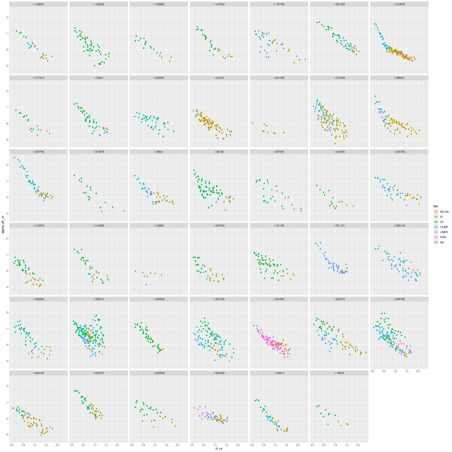
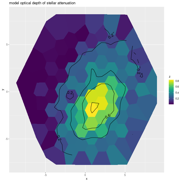
I’m returning now to the Leung et al. (2024, 2025) sample of post-starburst galaxies observed in MaNGA. I actually completed model runs for the entire sample some time ago, but it’s taken a while to examine the results and that is still underway. To summarize briefly the sample consists of 48 “central” (CPSB) and 41 “ring” (RPSB)1this classification scheme was proposed by Chen et al. 2019. See also Cheng et al. 2024. galaxies. I analyzed 1255 spectra from the CPSB sample and 2202 from the RPSBs. This was out of 5310 and 7755 spectra in the stacked RSS files that are the sources of my spectroscopic data. I generally tried to bin spectra to a minimum mean SNR of 8 per wavelength bin, although I sometimes accepted less. I excluded spectra that failed to meet whatever threshold I set as well as spectra with foreground star contamination: there were 1311 and 2311 binned spectra in the two subsamples, so I excluded 56 and 109 from analysis.
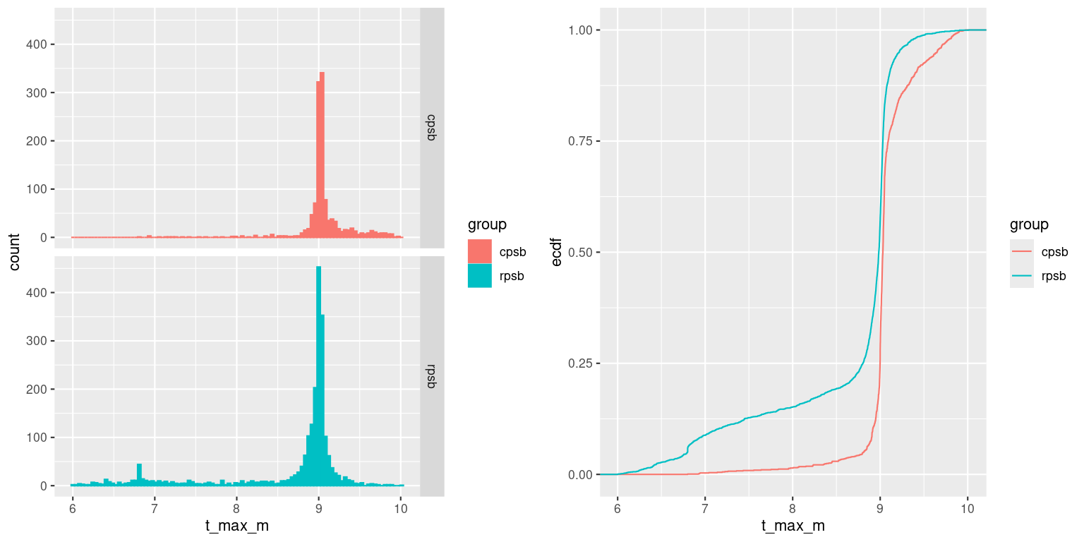
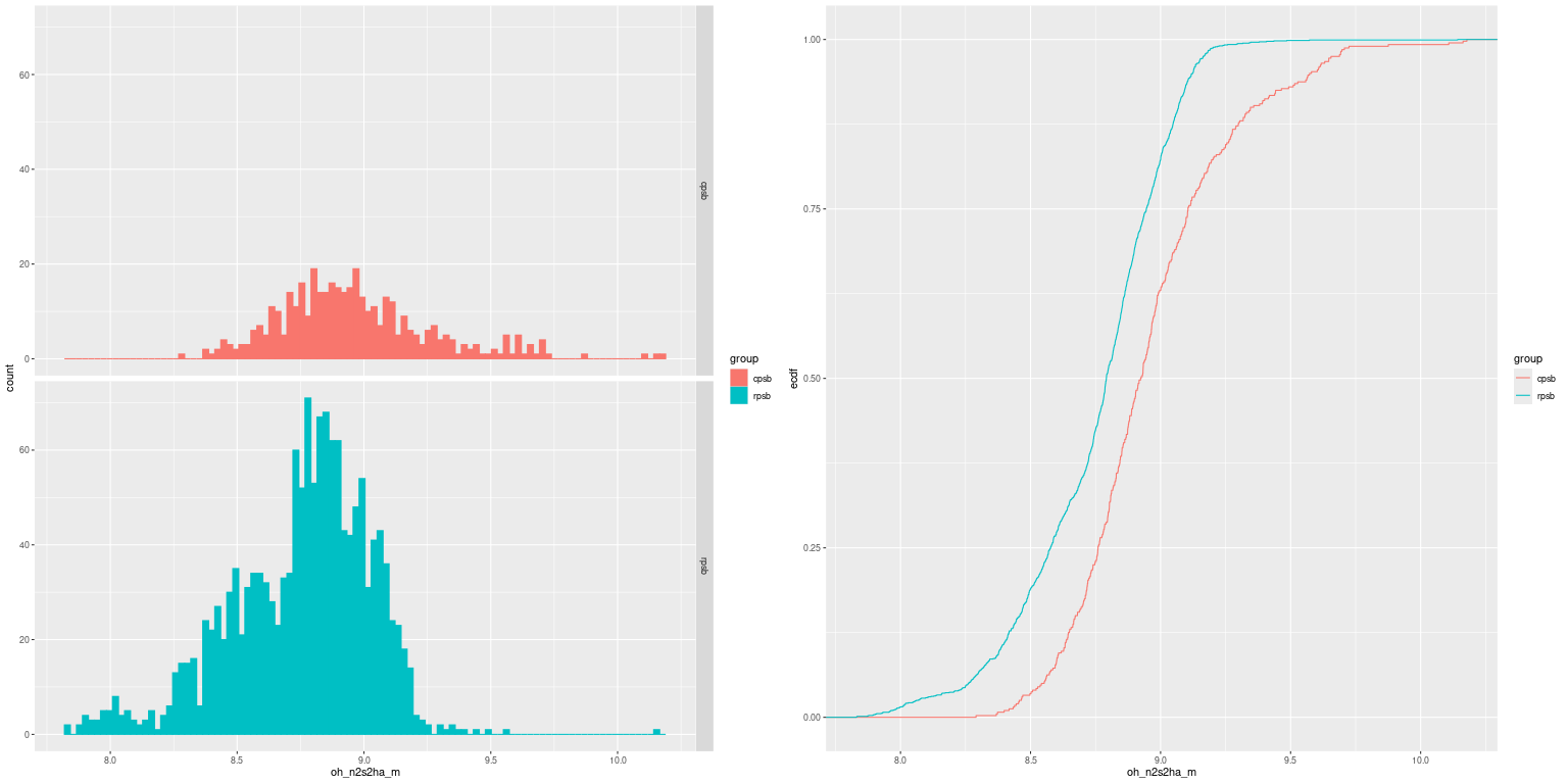
Some time ago while still running models for this sample I mentioned noticing a distinct tendency for model star formation rates to peak at right around 1 Gyr. Since then I’ve added measurements of the lookback time to maximum star formation rate, so I can now check if my visual impression was correct. And, as the graph below shows, it was! This displays on the left histograms of counts of lookback times to maximum SFR, and on the right empirical cumulative distribution functions for the two samples.
Lookback time to epoch of maximum star formation rate by PSB classification
Clearly both have very strong peaks right around 1 Gyr, which again raises the question whether this is a sample selection effect or something in the models or SSP library that’s preferentially producing large contributions from a narrow age range. I’m still investigating this and will follow up in a future post. As a preliminary comment model runs with the BPASS library for a few galaxies show a similar tendency to have very strong peaks but at earlier ages of ~2 Gyr.
The other striking thing here is that the RPSBs have a long tail of more recent peaks: about 5% of the regions are still star forming (peak SFR at < 107 yr) and 15% peaked < 100 Myr ago, while < 2% of CPSB regions peak at < 100 Myr. Standard emission line diagnostics are consistent2these are based on [N II]/Hα vs [O III]/Hβ with Kauffmann’s “composite” region:
No Em
Weak Em
SF
Comp
LI(n)ER
AGN
CPSB
6
62
1
9
16
6
RPSB
2
30
25
26
12
5
Percent of analyzed spectra in BPT diagnostic regions
Regions with LINER and even AGN like emission line ratios aren’t necessarily centrally concentrated, so we can’t infer the presence of AGN from line ratios alone (there are known optical AGN in both samples however).
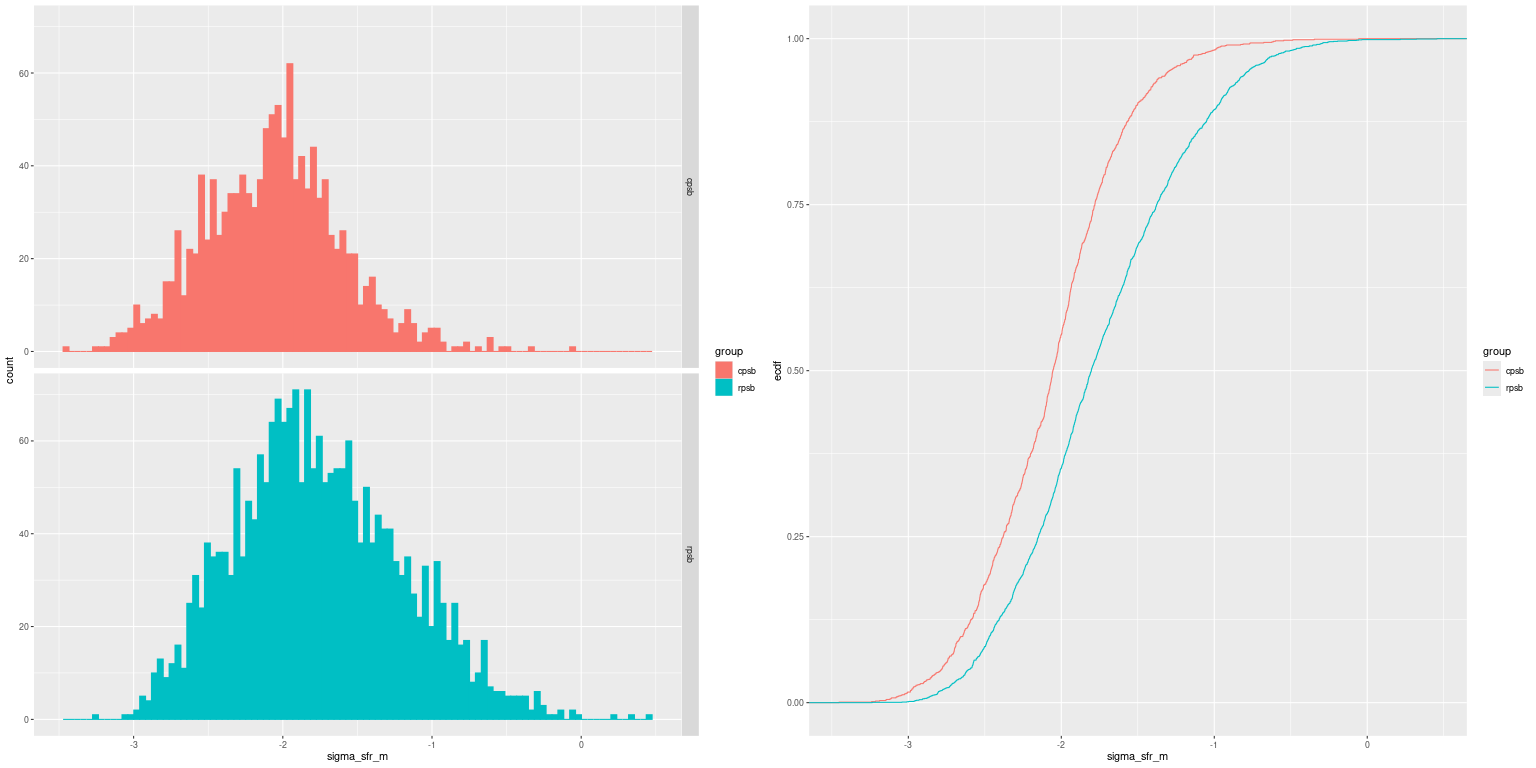
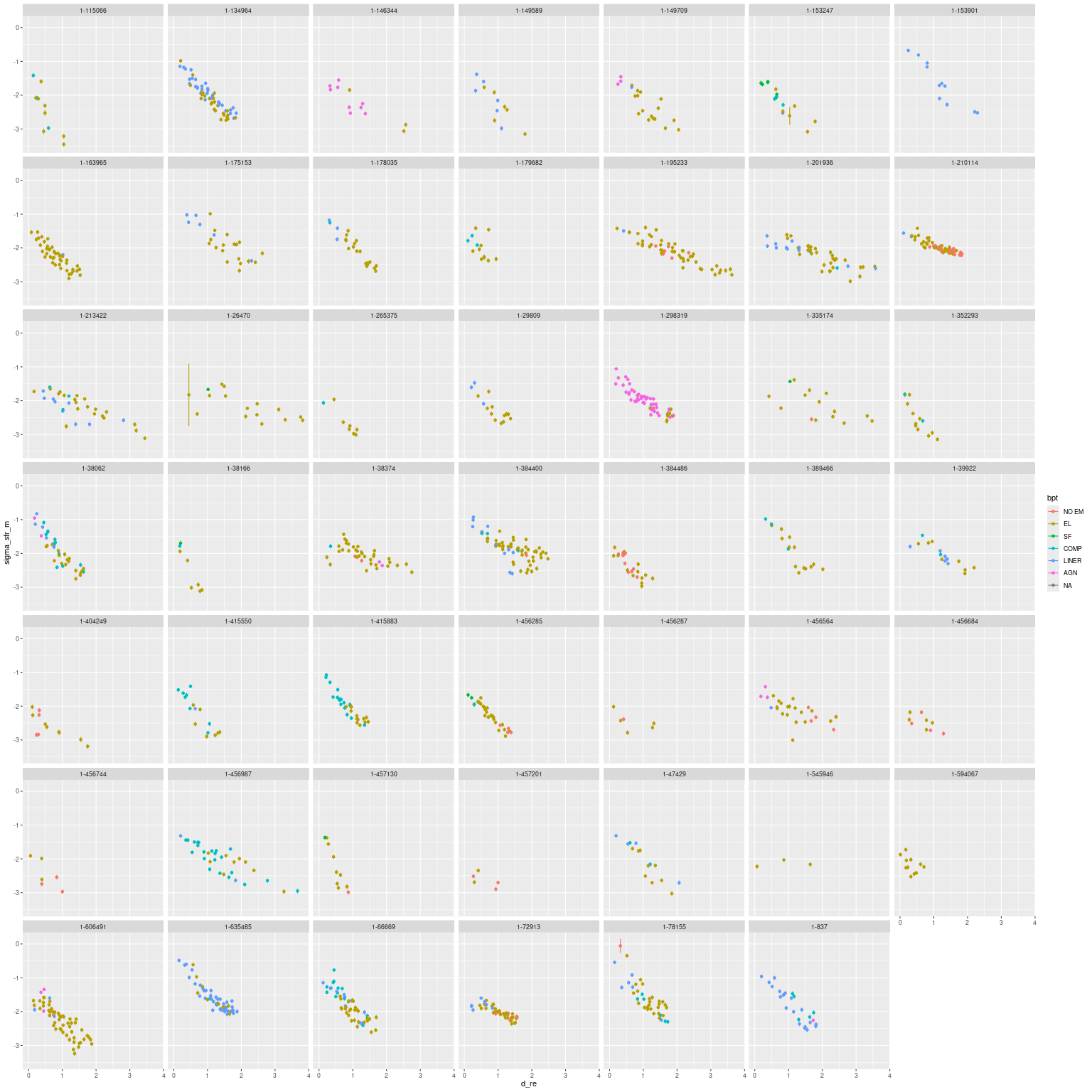
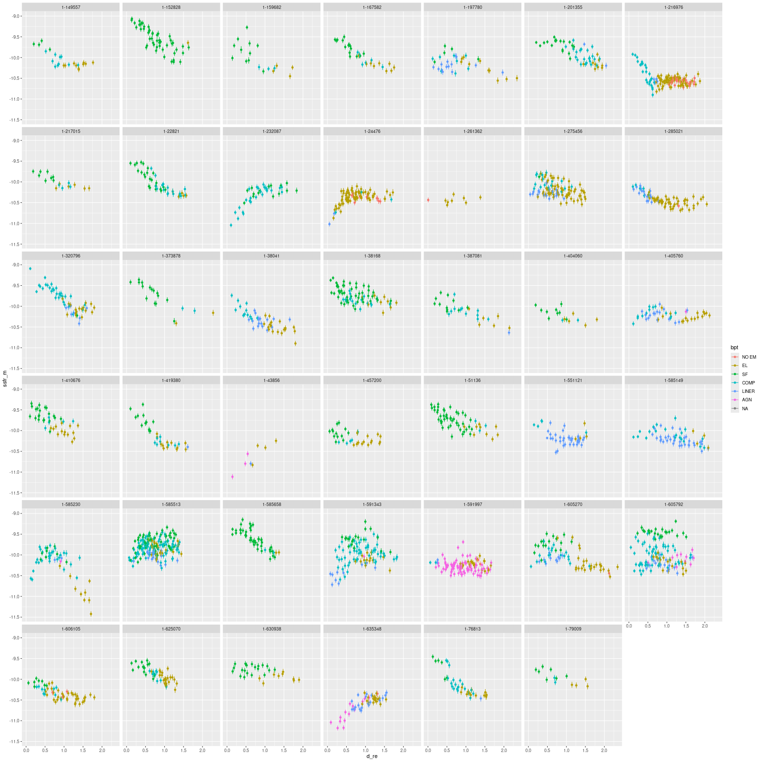
There are other population level differences as well. The RPSBs have higher (in distribution) star formation rate densities:
Distributions of 100 Myr average star formation rate density
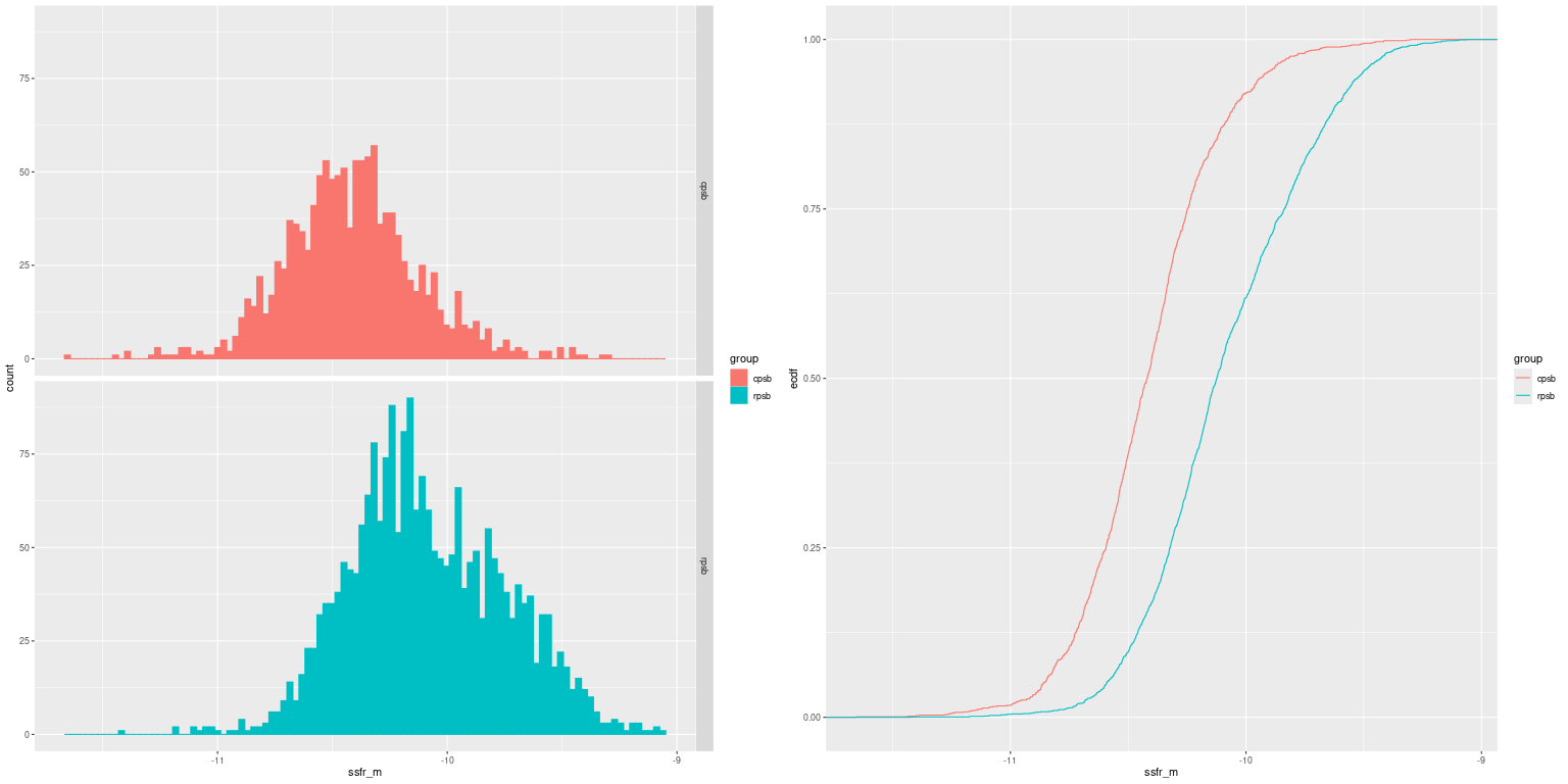
and specific star formation rates (both are 100 Myr averages):
Distributions of 100 Myr average specific star formation rate
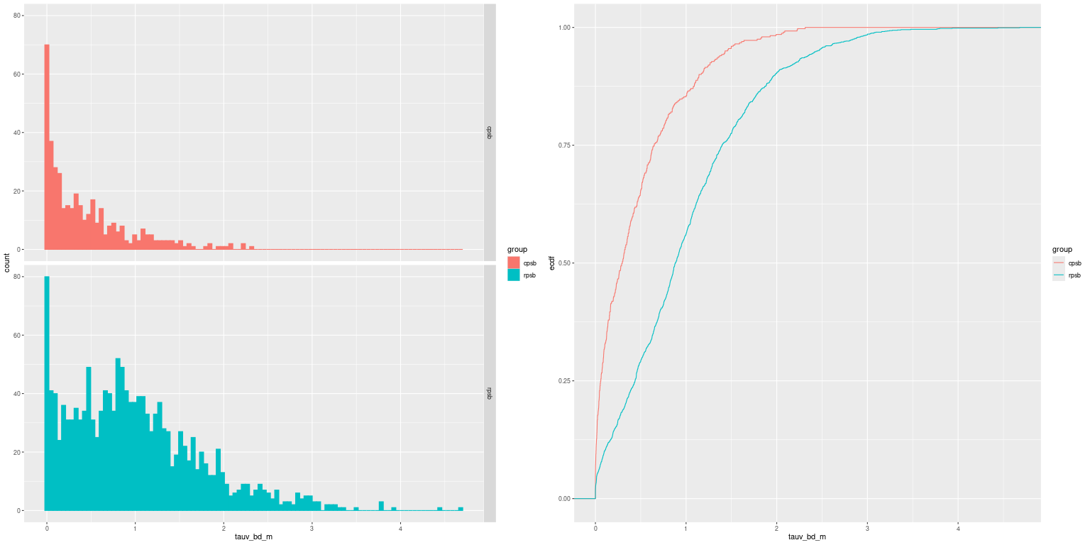
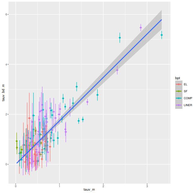
Limiting the samples to regions with firm emission line detections the RPSBs appear to be dustier:
Distributions of τV estimated from Balmer decrement (regions with firm detections only)
and have slightly lower gas phase metallicity:
Gas phase metallicity distributions from [N II], [S II], Hα diagnostic (regions with detections only)
For what it’s worth a Kolmogorov-Smirnov test says all of these empirical CDFs are different at essentially arbitrary significance levels.
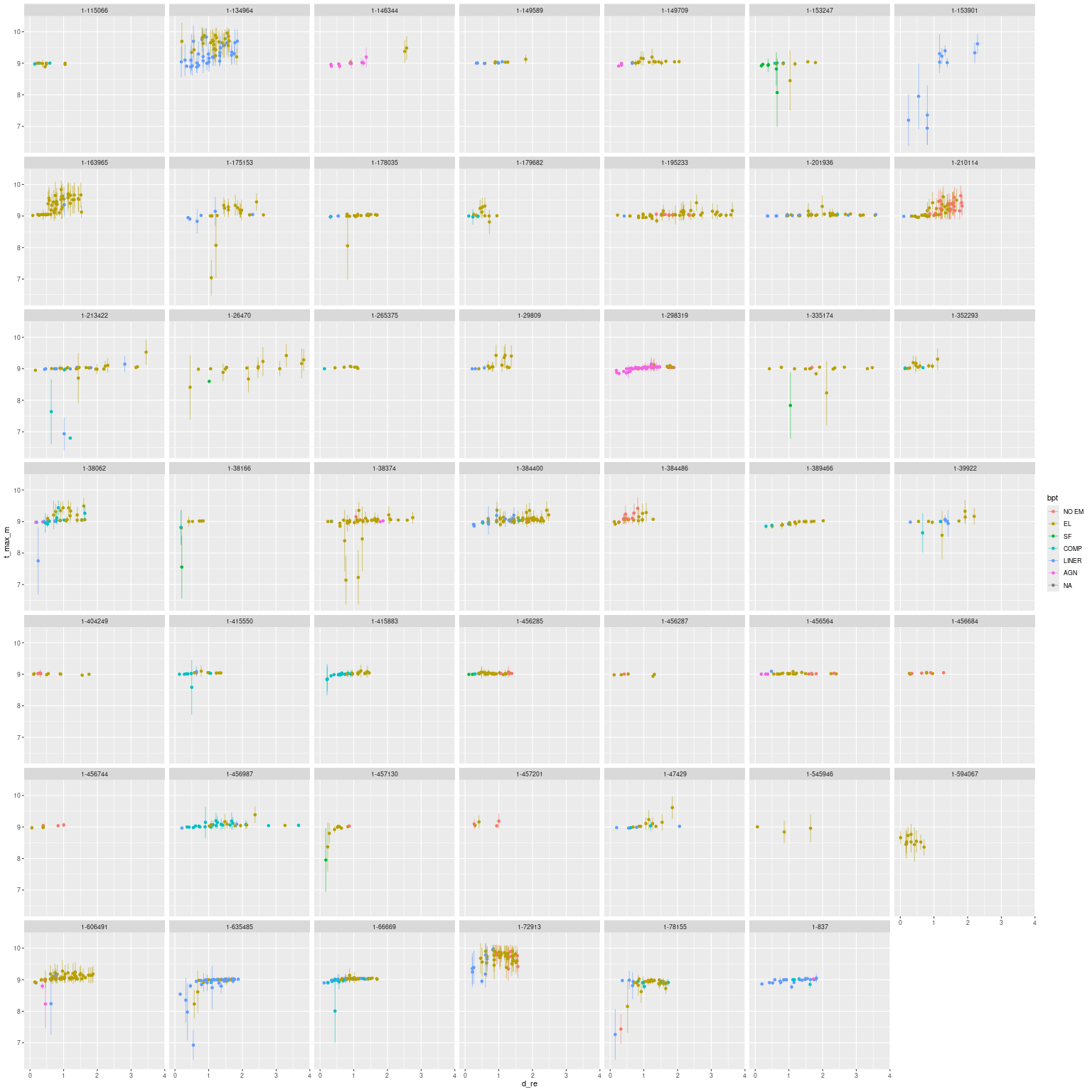
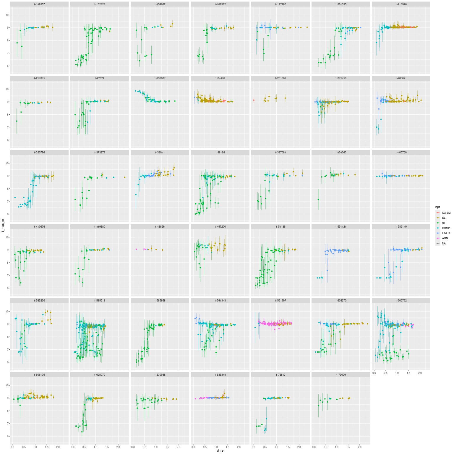
Turning to spatial variations of a few modeled quantities with projected radius for each galaxy and broken down by sample. First is lookback time to maximum SFR:
Lookback time to maximum SFR vs projected distance – CPSB sampleLookback time to maximum SFR vs projected distance – RPSB sample
The CPSBs generally have relatively constant burst ages with projected radius, with a small number having positive gradients — one of the better examples being mangaid 1-635485 (plateifu 7965-1902; row 7, column 2 in the plot above) that I discussed in the previous post. None have negative gradients (center significantly older than farther out).
The RPSBs on the other hand have many examples with positive age gradients. There are also a number of examples of star forming regions interspersed with post-starburst. There’s just one clear example (mangaid 1-232087, plateifu 8152-3703) with a strongly negative age gradient. My models have an old and quiescently evolving central region with a post-starburst disk.
Star formation rate density:
100 Myr average SFR density vs projected radius – CPSB sample100 Myr average SFR density vs projected radius – RPSB sample
sSFR:
100 Myr average sSFR vs projected radius – CPSB sample100 Myr average sSFR vs projected radius – RPSB sample
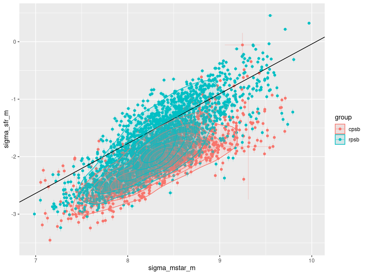
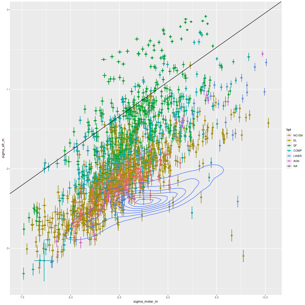
One final plot: (100 Myr averaged) SFR density vs stellar mass density. The solid line is my old calibration of the mean star forming main sequence (which I should recalibrate). Evidently the RPSBs have a larger fraction of regions in the star forming main sequence and conversely the CPSBs extend farther into the green valley.
ΣSFR vs ΣM* – CPSB and RPSB samples
Another thing I found rather odd about the Leung papers is they use some variation of the word “merger” 61 times in two papers, but there’s no indication that they actually examined imaging of their sample, all members of which are in both the SDSS and Legacy Survey footprints. I have examined the entire sample in Legacy Survey imaging3DR9 of Legacy Survey is considerably deeper than SDSS imaging using its custom catalog upload feature with the object list taken from the papers’ supplementary material. What I was mostly looking for was morphology, specifically morphological disturbance. What I found was an interesting difference between the two samples:
Merger
Merger remnant
Disturbed
Total
CPSB
1
7
2
48
RPSB
8
5
6
41
My count of systems with morphological disturbance. Based on visual examination of Legacy Survey imaging.
Almost half of the RPSBs have some level of disturbance, and there are 8 ongoing mergers (or perhaps flybys in a few cases). The mergers are in all stages of Toomre’s famous sequence ranging from M51/M52 like interacting pairs to fully merged systems with prominent tidal tails. There are also several merger remnants that are fully consolidated but with residual tidal tails, shells, and heavily disturbed overall appearance. This suggests either that mergers play a more important role in forming RPSBs, or alternately that we are simply seeing earlier stages of the transition to quiescence in them. I favor the latter: star formation has almost completely shut down in the CPSB sample, while it’s relatively widespread in the RPSBs.
I may return to take a closer look at “interesting” systems, especially the mergers. After that I may look at extending the models somewhat, in particular to include kinematics in the Bayesian part of the analysis.
I am now, finally, going to turn to the properties of the stellar populations within the IFU footprint and detailed star formation history models. As a reminder these are based on my longstanding Stan language based code for nonparametric SFH modeling using what I refer to as the “medium” ProGeny based SSP model library as stellar inputs.
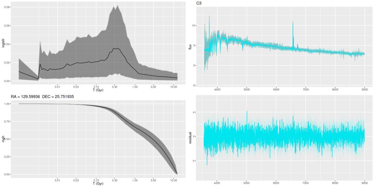
There are several distinct regions of interest, and I’ve taken the liberty of grabbing a screenshot from a figure in Cortijo-Ferrero et al. (2017) for orientation. The central region generally outlined by the Hα contour lines has the highest stellar mass density and ongoing star formation. The 3 H II regions marked C1, C2, and C3 are clearly seen in the emission line maps in my previous posts.
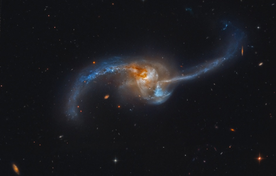
The wedge shaped region in the south that looks relatively blue in optical wavelength color images will turn out to be especially interesting. In the merger models of Privon, Barnes et al. (2013) the material in what Mulia, Chandar, and Whitmore (2015) call the “pie wedge” belongs to the progenitor that formed the northeastern tidal tail and constitutes the base of the tail that is now falling back into the main body of the merger remnant. As we will see the wedge contains most of the post starburst regions in the galaxy. There are also post starburst regions in a chain of bright clumps mostly west and north of the nucleus.
Screenshot of HST image of NGC 2623 with Hα contours overlaid from Cortijo-Ferrero et al. 2017.
There have been a number of attempts to characterize the stellar populations of this galaxy. In a probably non-exhaustive literature review I found 4 that used HST multiband imaging and aperture photometry to estimate the ages of clusters in the tidal tails and wedge: Evans et al. 2008, the aforementioned Mulia, Chandar and Whitmore 2015, Linden et al. 2017, and Cortijo-Ferrero et al. 2017. All of these used broad band color-color diagrams and various versions of BC03 SSP models for age estimates, which is evidently not very precise and highly degenerate with dust reddening. Fortunately the pie wedge region has very low attenuation in my models (τV ≲ 0.25). Nevertheless there’s a wide range of estimates in these works. Evans estimated ages of ~1-100 Myr for clusters in the pie wedge. Mulia also found ages of ~100 Myr, claiming that much of the observed scatter was due to photometric errors. They also estimated the age of the diffuse light, finding a somewhat older age of ~500Myr. Linden et al. found a wide range of ages from 3.5-350Myr in just 11 clusters in the pie wedge and the bright clumps west of the nucleus. In an appendix to their mostly CALIFA based study Cortijo-Ferrero used archival HST images to estimate cluster ages to the south of the nucleus in the range 100-400 Myr, with an average ~250 Myr.
There have been 4 IFU based spectroscopic studies that I have found. The study by Lipari et al. that I discussed in the previous two posts exclusively considered emission line properties. Medling et al. (2014) performed a near IR study using an instrument named OSIRIS primarily directed at stellar and gas kinematics. The spatial coverage of their observations was only ~500pc, which is smaller than a MaNGA fiber so their work is not directly relevant. One interesting result is they found the nuclear stellar population to have a mean age ~30Myr.
I already mentioned the CALIFA based study of Cortijo-Ferrero et al. A second paper in the series (Cortijo-Ferrero et al. 2017) performed a comparative study of several (U)LIRGs. Their work is the most similar in objectives and to some extent methodology to mine. I’ve only found two studies concerning stellar population properties using MaNGA observations. Kauffmann et al. (2024) found strong evidence for a population of Wolf-Rayet stars in the circumnuclear region, which would prove the presence of a recent or ongoing nuclear starburst. As I mentioned a few posts ago this was a candidate “Central Post Starburst Galaxy” in the work by Leung et al. For reasons that I may get around to discussing later they chose not to analyze it as part of their final sample.
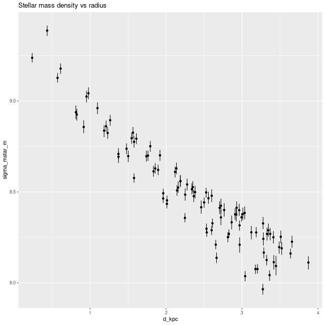
Turning to my own model results I’ll first look at some large scale properties, in no particular order. The stellar mass density peaks just to the east of the nucleus, approximately at the position of the cluster aggregation marked “A” in the HST based image above. The trend with radius appears to be close to exponential, suggesting this system is still disky.
NGC 2623 (MaNGA plateifu 9507-12704) – (L) map of model stellar mass density/ (R) Stellar mass density vs. distance from nucleus
The stellar dust attenuation also peaks just east of the nucleus. Given the complex dust geometry it’s possible my simple one component attenuation model is failing here: if the light is dominated by young stars still in their “birth cocoons” and the model fits the attenuation to them it will tend to overestimate the mass in older stars. This may be a case where I’d be justified in running a model with two dust components.
In the south the area of the pie wedge has mostly very low attenuation, as do the bright clumps south and west of the nucleus.
NGC 2623 (MaNGA plateifu 9507-12704) – Model stellar attenuation
I estimate the total stellar mass within the IFU to be ≈ 4×10¹⁰ M☉ (log(M*) = 10.617 ± 0.0071which is wildly overoptimistic. This is just a sum over all individual estimates, which should overstimate the total by about 0.2 dex since the fiber positions overlap. However the IFU doesn’t quite cover the full visible extent of the main body and almost none of the tidal tails, which will add perhaps a similar amount to the total. This estimate appears within the range I’ve found in the literature. For example Shangguan et al. (2019) give an estimate of log(M*} = 10.60 ± 0.2 (for future reference they estimate the star formation rate to be log(SFR) = 1.62 ± 0.04). The previously cited Cortijo-Ferrero et al. (2017) estimate it to be 2.4 x 10¹⁰ M☉ with Chabrier IMF. Howell et al. (2010) estimated the stellar mass as 6.42×10¹⁰ M☉ (log(M*) = 10.81) and the star formation rate at 69.19 M☉/yr based on IR/UV photometry. The NASA Sloan Atlas catalog, which serves as the source for derived quantities in the MaNGA DRP estimates the stellar mass to be 3.1 – 3.4×10¹⁰ M☉.
NGC 2623 (MaNGA plateifu 9507-12704) – Total stellar mass within IFU.
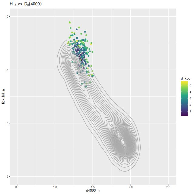
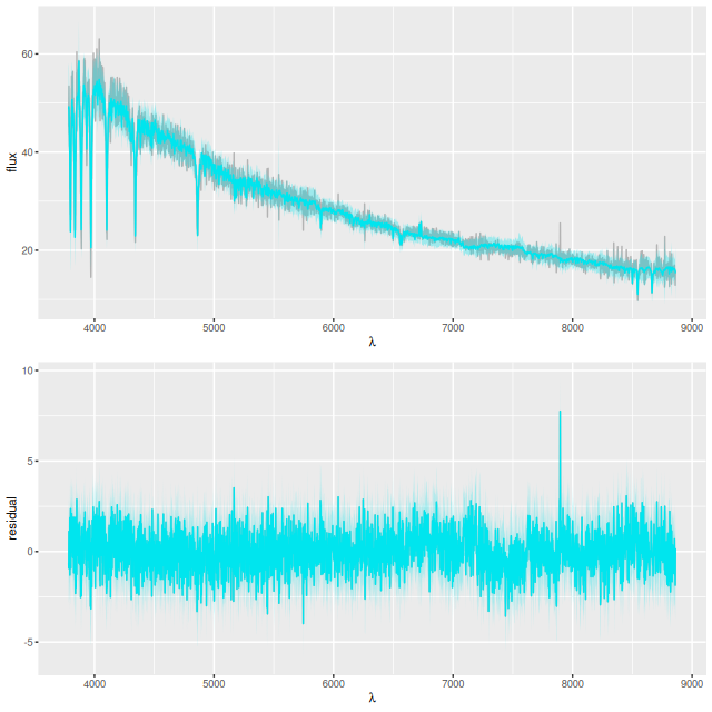
A popular absorption line diagnostic, and one I’ve displayed several times, is a plot of Balmer line strength versus the 4000Å break strength. Although it doesn’t uniquely constrain the evolutionary state of a system it does give some rough idea of the contribution of intermediate mass stars and the mean stellar population age. Plotted below are the Lick HδA index and Dn(4000). The contour lines are for a large fraction of SDSS galaxies measured by the MPA-JHU pipeline. Note that many of the points are above the last contour line in the region, which indicates a significant fraction of the galaxy is in a post-starburst state.
NGC 2623 (MaNGA plateifu 9507-12704) – plot of H&deltaA versus 4000Å strength Dn(4000).
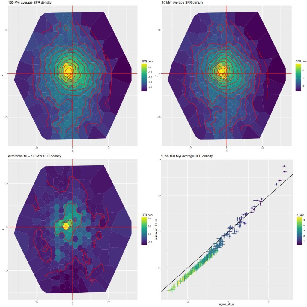
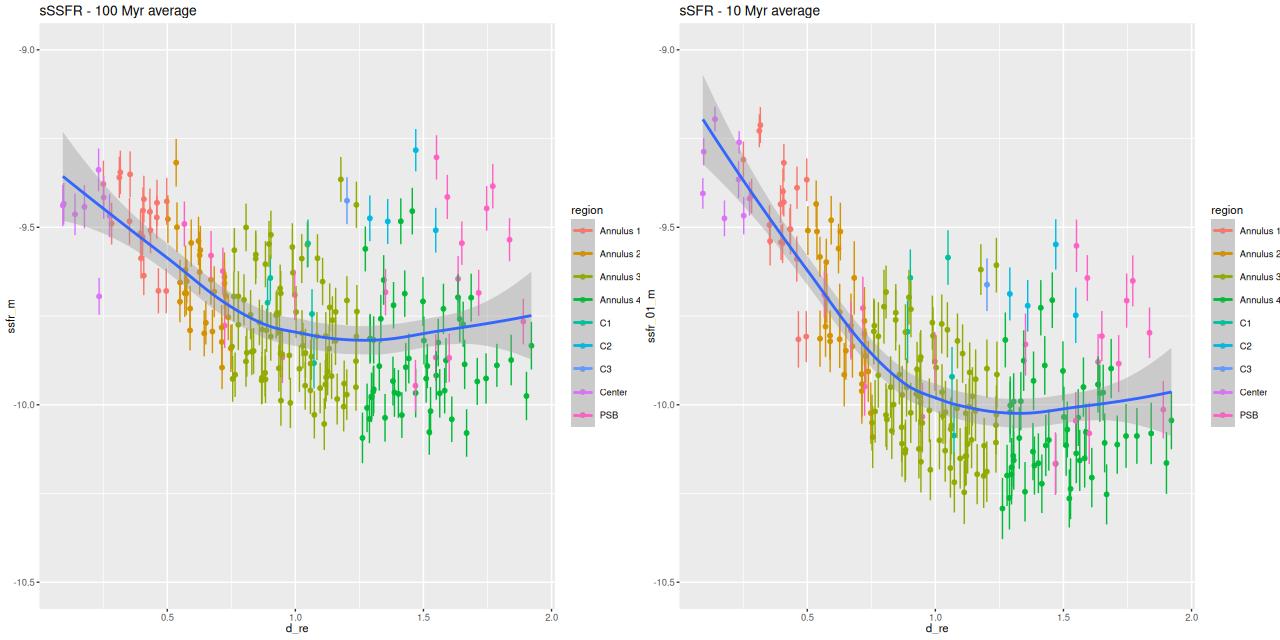
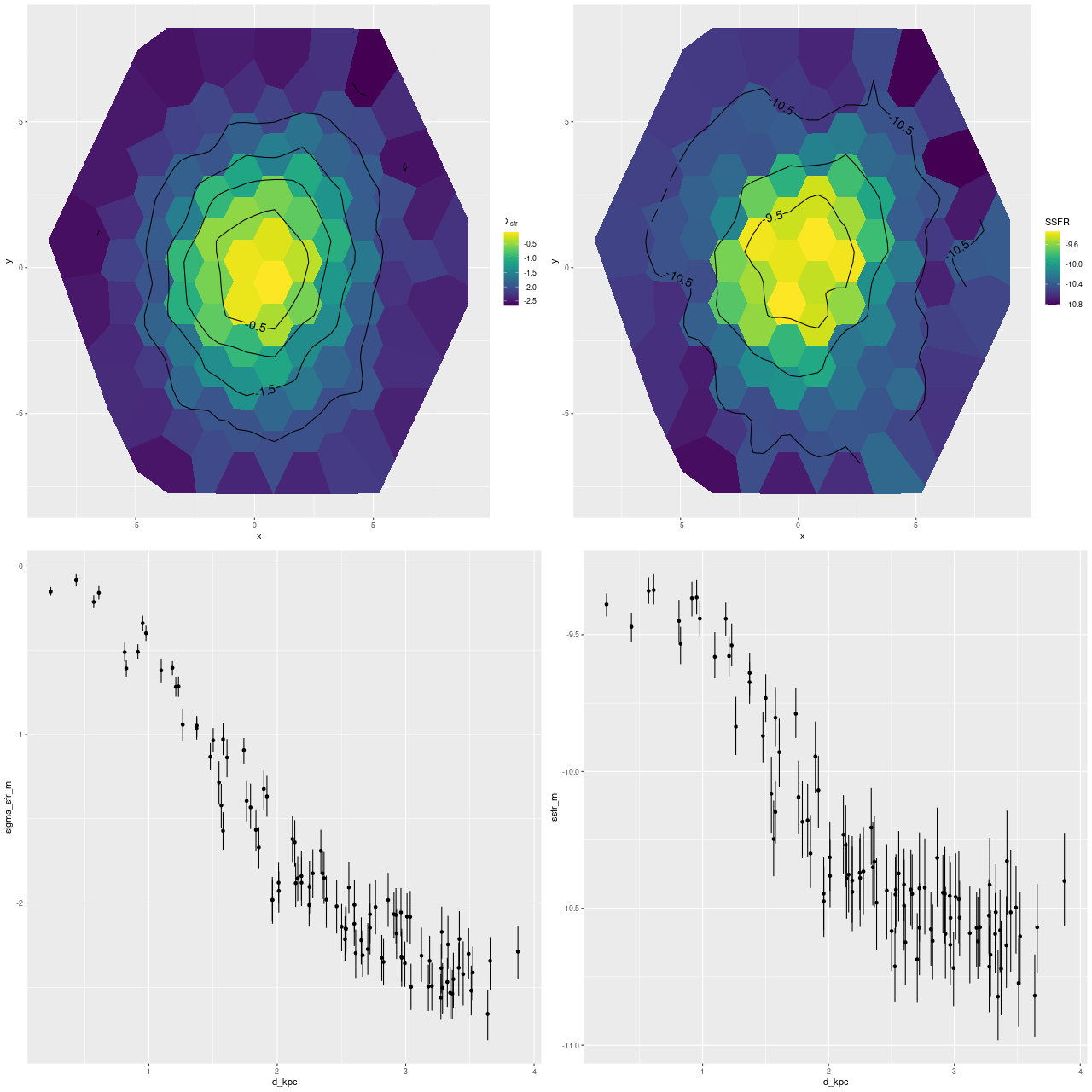
Part of my post-processing of models are calculations of star formation rate surface densities log10(ΣSFR) in units of M☉/yr/kpc2 averaged over a preselected lookback time interval. I’ve always used 100Myr as that interval, mostly because it’s a nice round number that’s often used in the literature. This time I decided to do also a calculation for a 10Myr lookback time, which is about the timescale for estimates based on Hα luminosity. The results are shown below: the top row are the estimates, and the difference is in the bottom left. As can be seen in the scatterplot at bottom right a small region near and just east of the center has had a recent increase in star formation, while it’s remained nearly constant out to about 1.5 kpc (~ 1/2 reff) and has declined farther out.
NGC 2623 (MaNGA plateifu 9507-12704) – Top row – model mean star formation rate density averaged over 100 and 10 Myr intervals (logarithmically scaled). Bottom left: difference between 10 and 100 Myr averages. Bottom right: scatter plot of 10Myr SFR density vs. 100Myr.
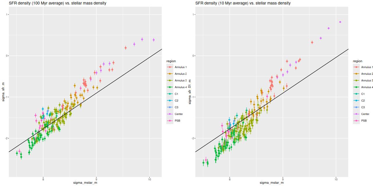
Finally, here is another standard visualization of the relation between star formation rate density and stellar mass density. The left panel is the 100 Myr averaged SFR density while the right is 10 Myr. The straight line is my estimate of the mean “spatially resolved star forming main sequence.” This was done some time ago with a sample of normal starforming disk galaxies and the EMILES + Pypopstar SSP library and should probably be recalibrated. Comparing the two plots it’s apparent that some regions are evolving into the “green valley” while others have evolved into the starbursting region.
NGC 2623 (MaNGA plateifu 9507-12704) – SFR density vs. stellar mass density. (L) 100 Myr average. (R) 10 Myr average SFR density. Straight line is my estimate of the “spatically resolved star forming main sequence.”
Star formation rate histories by region
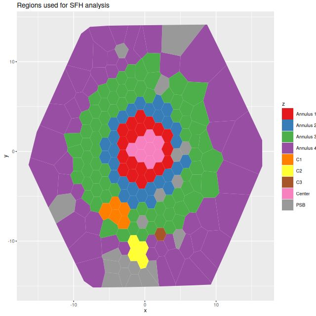
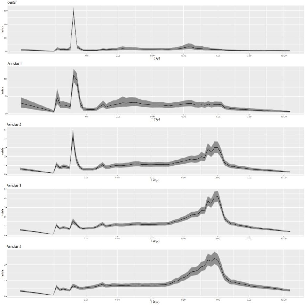
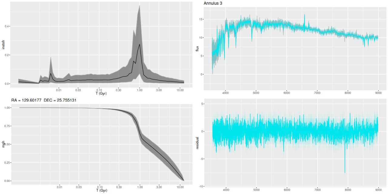
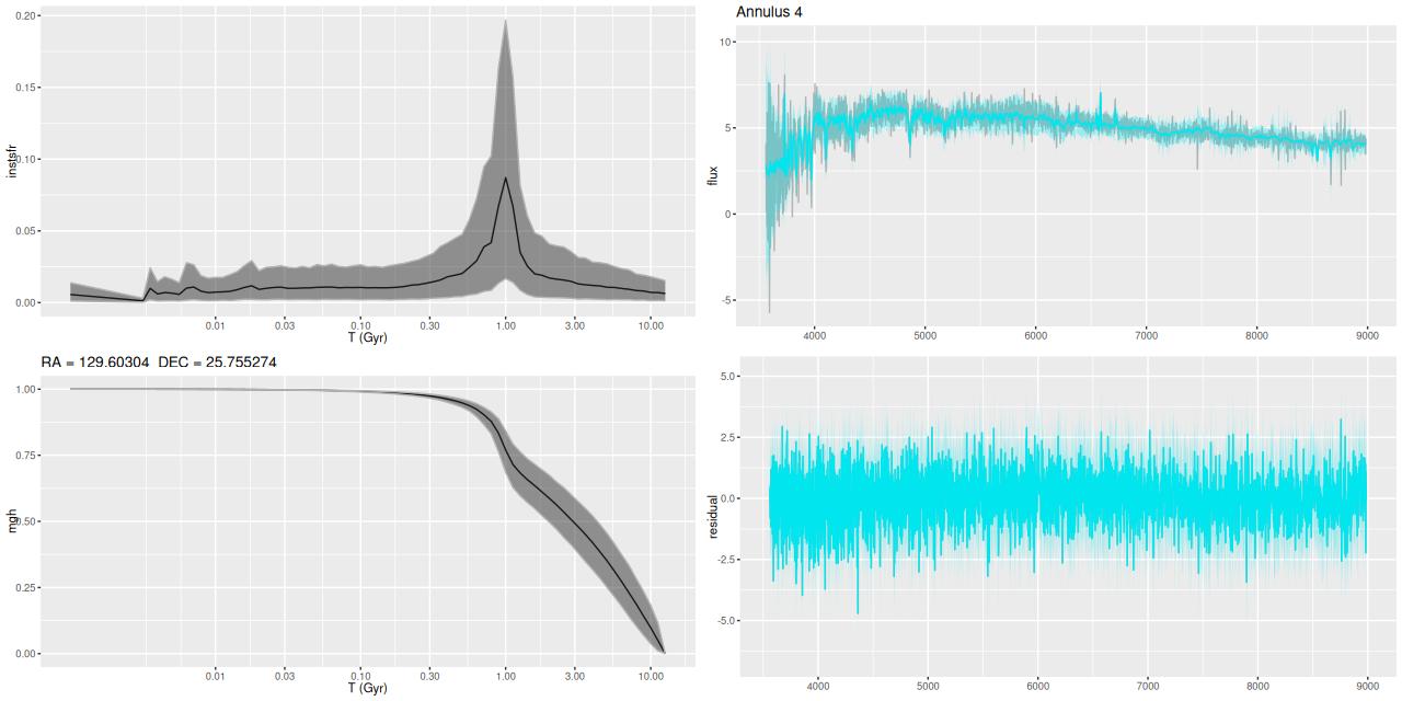
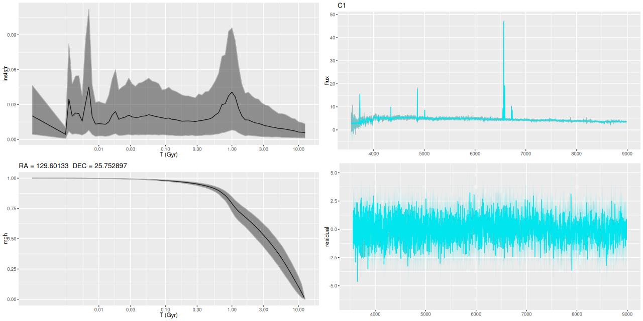
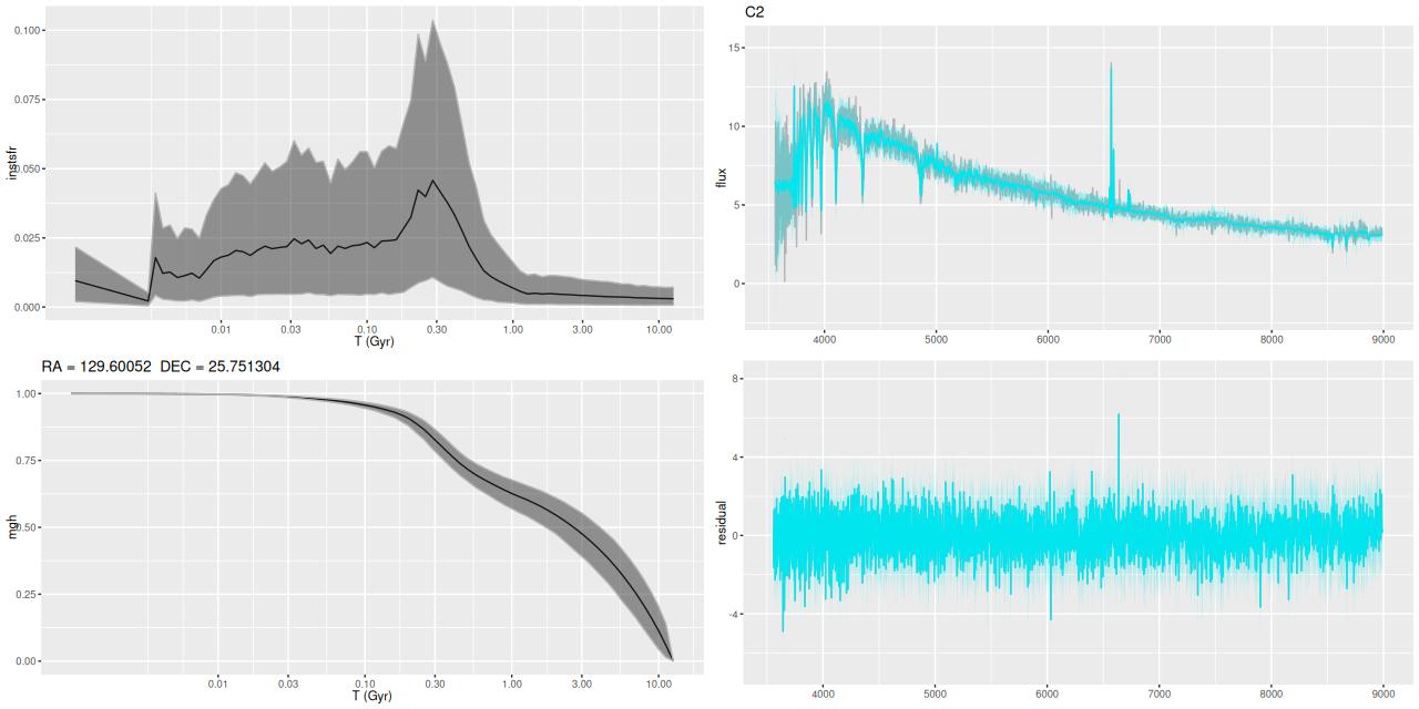
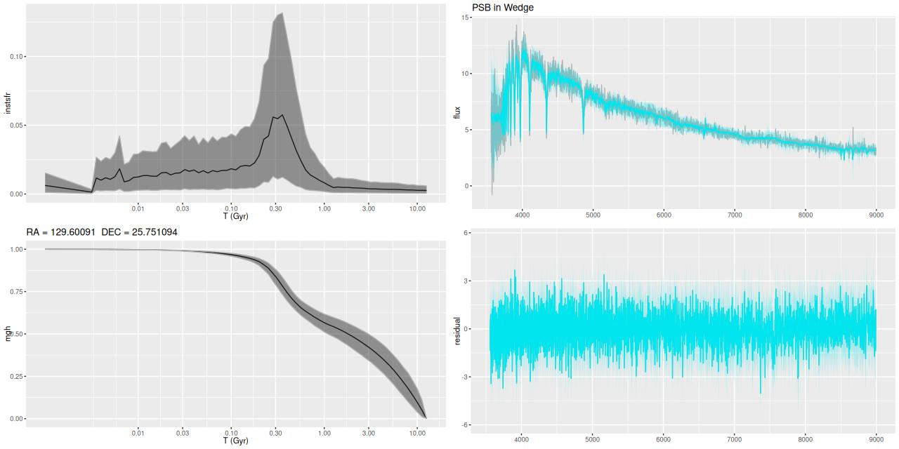
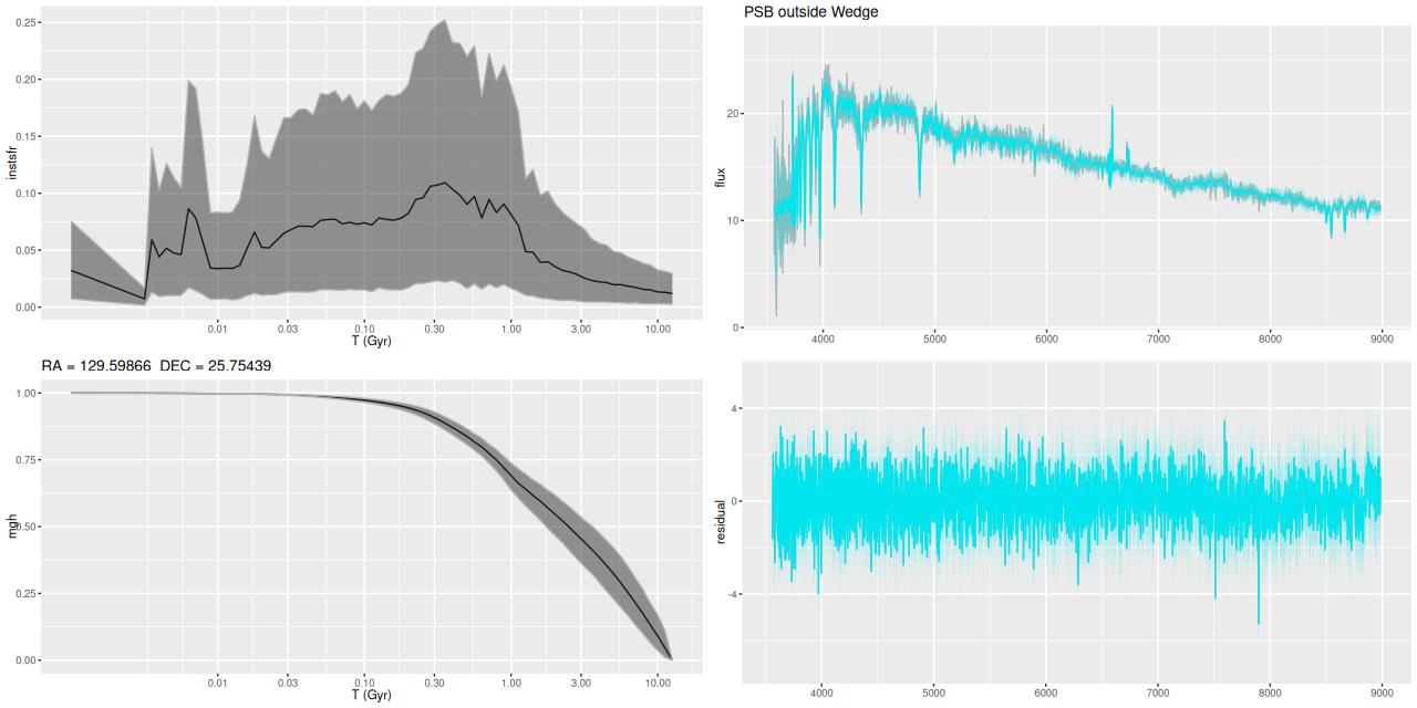
Next I’m going to present detailed star formation rate histories for the entire IFU footprint. The stacked RSS spectra binned to 214 with SNR ≥ 8.5, which is a few too many to display individually. As we’ve seen there are at least 3 distinct regions with likely different recent star formation histories: the circumnuclear region has a central starburst and at least two large star cluster complexes; farther out there are 3 separate areas with star forming emission line ratios and enhanced Hα fluxes relative to their surroundings; the “pie wedge” has many star clusters with estimated ages ~100Myr and post-starburst spectra. Some of the bright clumps seen to the west of the nucleus also have post-starburst spectra. For display purposes I’ve made a slightly finer grade division as follows:
Center region: the closest fiber to the center and its immediate neighbors including cluster aggregation “A” to the east. (see top of post). This covers most of the region with highest emission line flux.
Annulus 1: regions with D ≤ 0,5 reff (I adopted reff = 7.9″ ≈ 2.9 kpc from the NSA atlas) and outside the center region.
Annulus 2: 0.5reff < D ≤ 0,75 reff, excluding regions with post-starburst spectra.
Annulus 3: 0.75reff < D ≤ 1.25 reff, excluding regions with post-starburst or starforming spectra.
Annulus 4: D > 1.25 reff, excluding regions with post-starburst or starforming spectra. The maximum IFU coverage is 2reff.
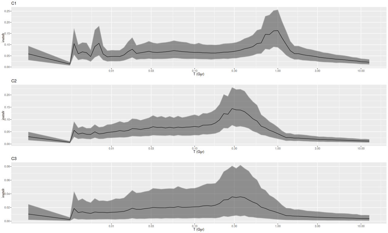
I chose to display the 3 regions of H II aggregations separately. The first is the one labelled “C1” in the graphic at the top of the post.
H II region(s) “C2”
H II region(s) “C3”. Both of these lie at the edge of the “pie wedge.”
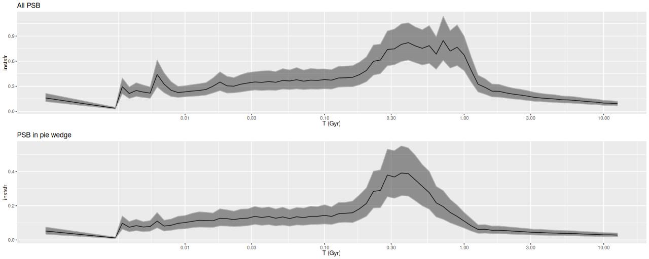
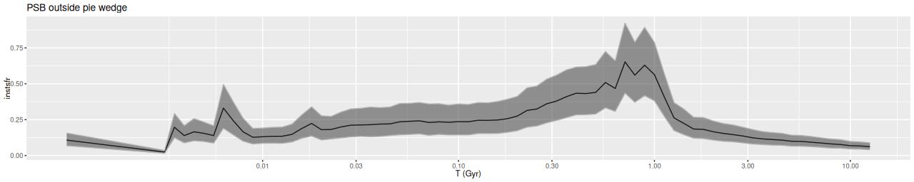
Visual examination of the spectra showed that many of them have classic A+K like spectra, with very strong Balmer absorption and weak emission (this was known some years ago: see Liu and Kennicutt 1995). I made a PSB region selection with highly stringent criteria:
Lick HδA – 2σ(HδA) ≥ 6.25Å
BPT class of “EL” or “NO EM” (i.e. weak or no emission lines detected). I used this instead of the more traditional equivalent width criterion mostly because I haven’t validated my EW calculations.
Essentially all of the “pie wedge” meets these criteria, as do several bright clumps west of the nuclear region. With relaxed selection criteria much of the galaxy outside the circumnuclear region could qualify by, for example Alatalo‘s criteria for “Shocked POststarburst Galaxies.”
NGC 2623 (MaNGA plateifu 9507-12704) – Distinct regions used for aggregated SFH model plots. Note that the post starbursts are in several disconnected regions.
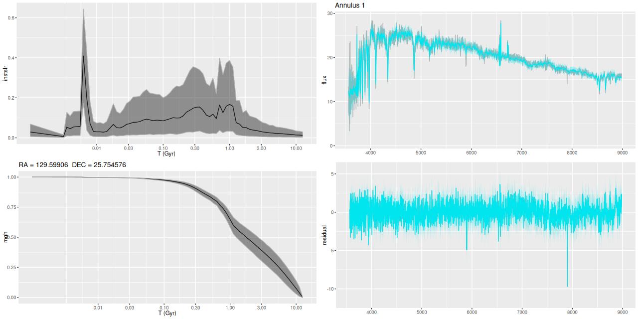
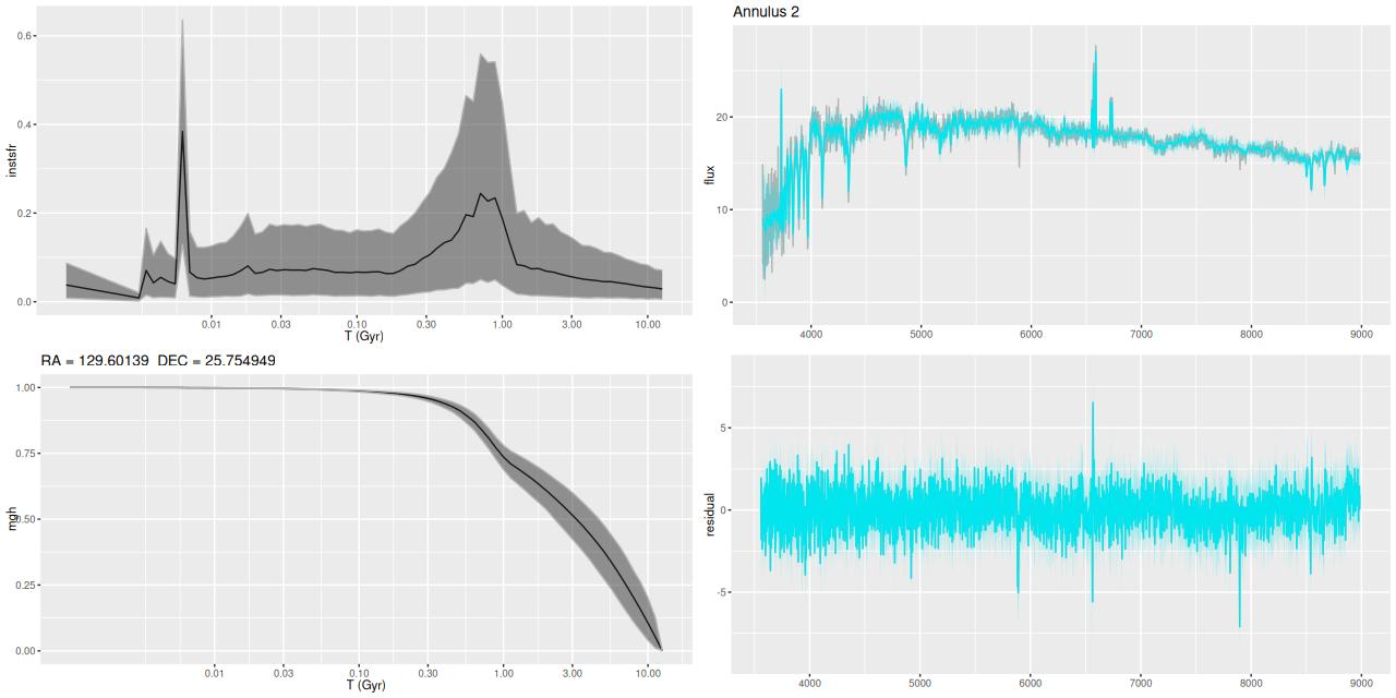
Modeled SFR histories are shown below grouped into 3 sets. The horizontal axes are logarithmically scaled, while the vertical axes are linear with different scales for each plot. Units are M☉/yr; these are estimated by summing over all models for the binned spectra comprising each group.
SFH in annuli
Star forming regions
Post starburst regions and the “pie wedge”
To summarize my visual impressions, star forming appears to have accelerated beginning ≈1 Gyr ago. In what is now the main body of the galaxy it plateaued shortly thereafter and then slowly decayed until very recently (< 10 Myr) where we are seeing a centrally concentrated starburst with declining star formation in the outskirts of the main body.
In the pie wedge including the two starforming regions the peak was much later at ≈300 Myr, and again with a subsequent slow decay. The only difference between the starforming and PSB regions of the wedge is the former evidently still have enough residual star formation to power H II regions. The PSB regions outside the pie wedge have a much different SF history from those inside it, with an early peak at ~1 Gyr and slow decay, much like the rest of the galaxy outside the center. The broad plateau in the first of the PSB plots is therefore a bit of an illusion.
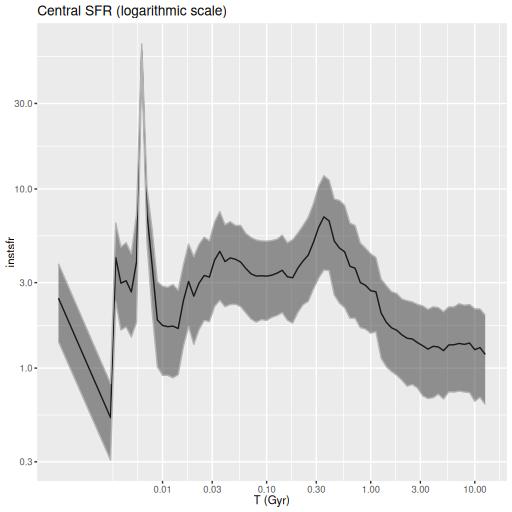
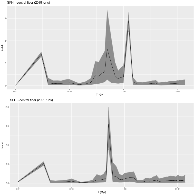
Although it’s obscured by the current starburst the central region also had a peak at ≈300 Myr.
NGC 2623 (MaNGA plateifu 9507-12704) – model star formation history in central region. Logarithmically scaled SFR
The 300 Myr peak is consistent with Privon et al.’s estimate of a first pericenter passage at ~220 Myr ago as well as the HST based estimates of star cluster ages in the wedge. However coalescence at ~85 Myr ago seems to have had no effect on star formation in my models — this is in contrast to most recent merger simulations, which typically have a strong centrally concentrated starburst around the time of coalescence. The large scale enhancement of SFR beginning at ~1 Gyr is also a bit puzzling. If the model is correct the effects of the interaction began well before the merger was underway.
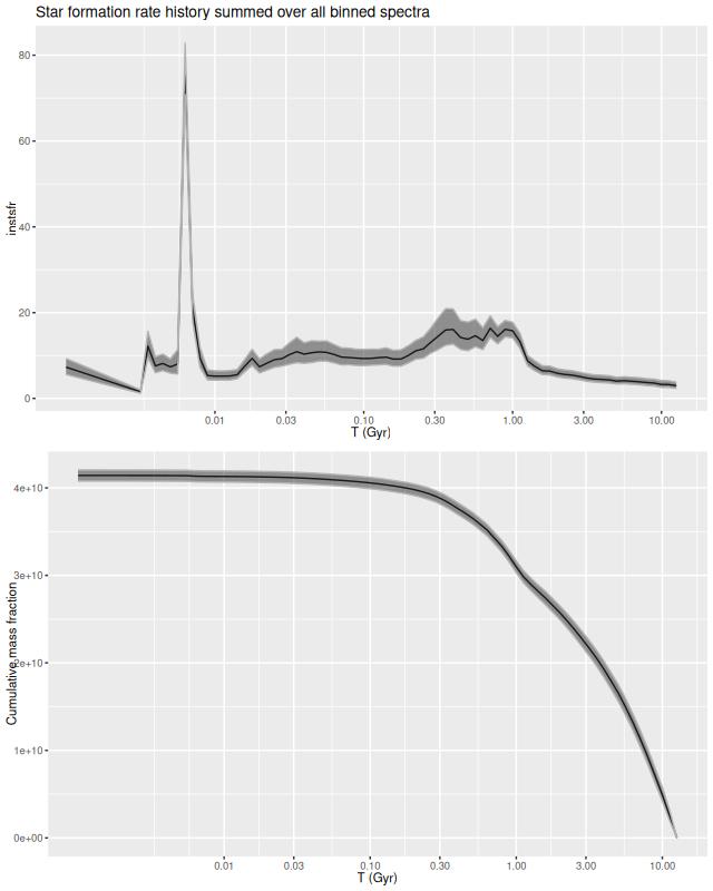
Finally for this section, here is the model star formation history summed over all 214 individual models. System wide there was a broad plateau from ~! Gyr to ~300 Myr ago, with a slow decline until ~10 Myr. The recent starburst only adds about 0.3% to the present day stellar mass, ~108 M☉.
NGC 2623 (MaNGA plateifu 9507-12704) – Model star formation rate history and mass growth history summed over all models for all binned spectra.
Selected individual SFH models
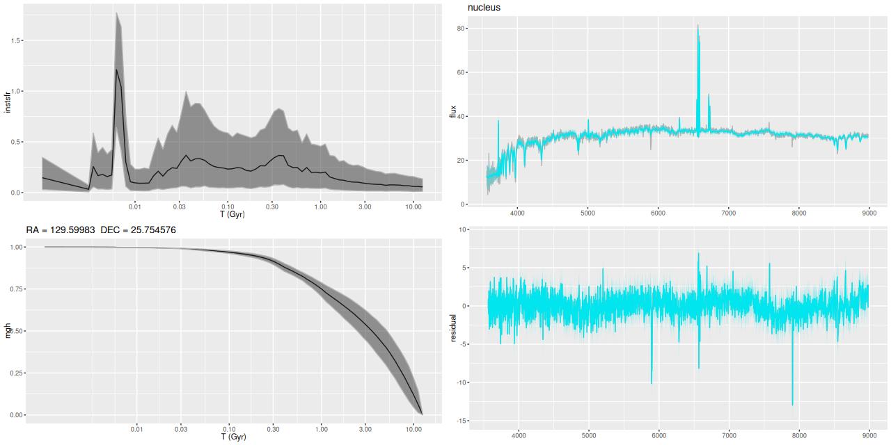
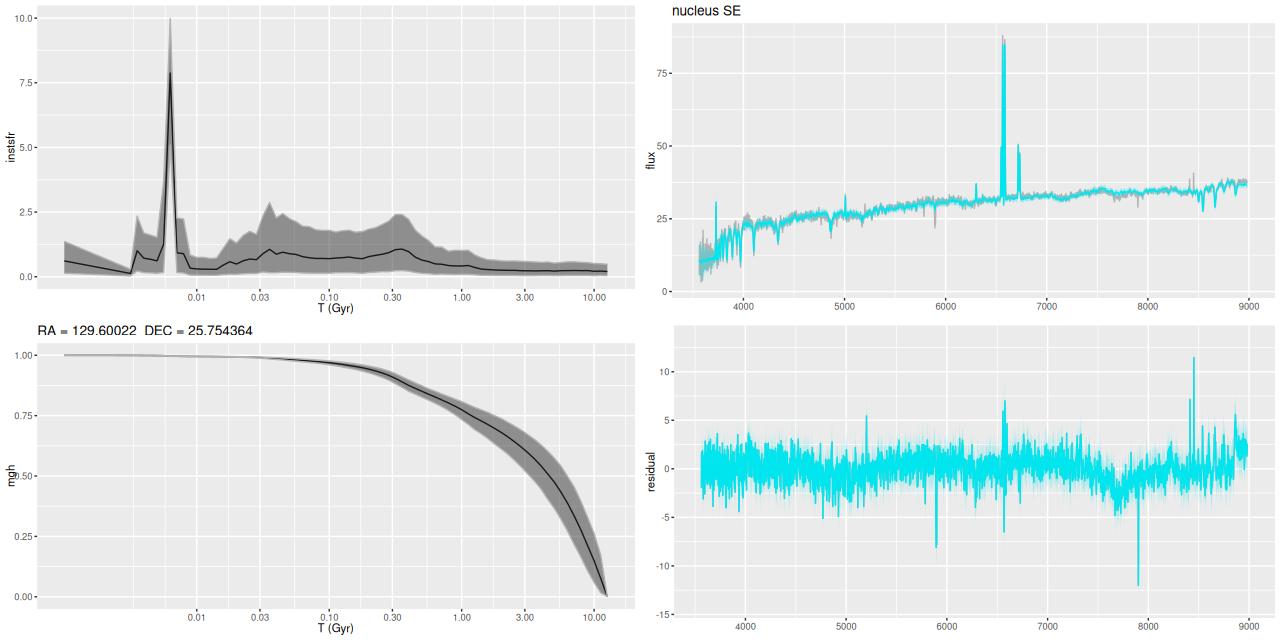
Plotted below are model star formation histories and fits to the data for 13 individual spectra, with the same ordering by region as the previous subsection. All horizontal scales are the same: lookback times are logarithmically scaled in Gyr; wavelengths are rest frame and cover the range of the model fits, which is ≈3560-9000Å. Vertical scales are linear with ranges chosen to cover the values plotted in each model run. The SFH plots include the position of the fiber center.
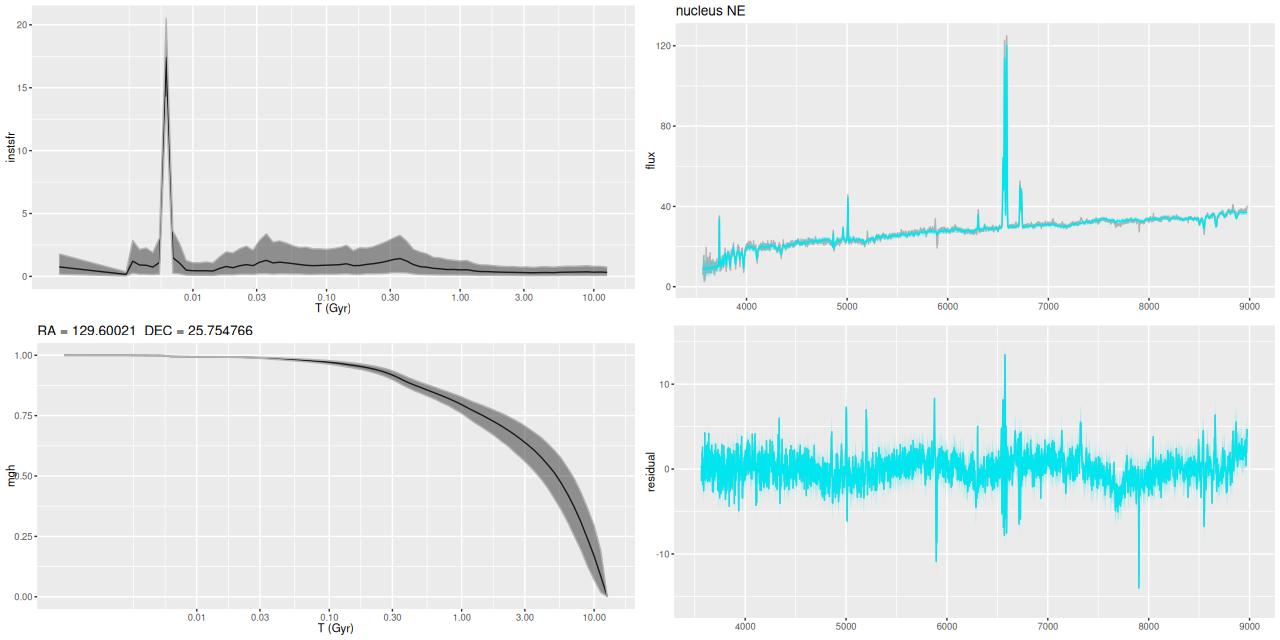
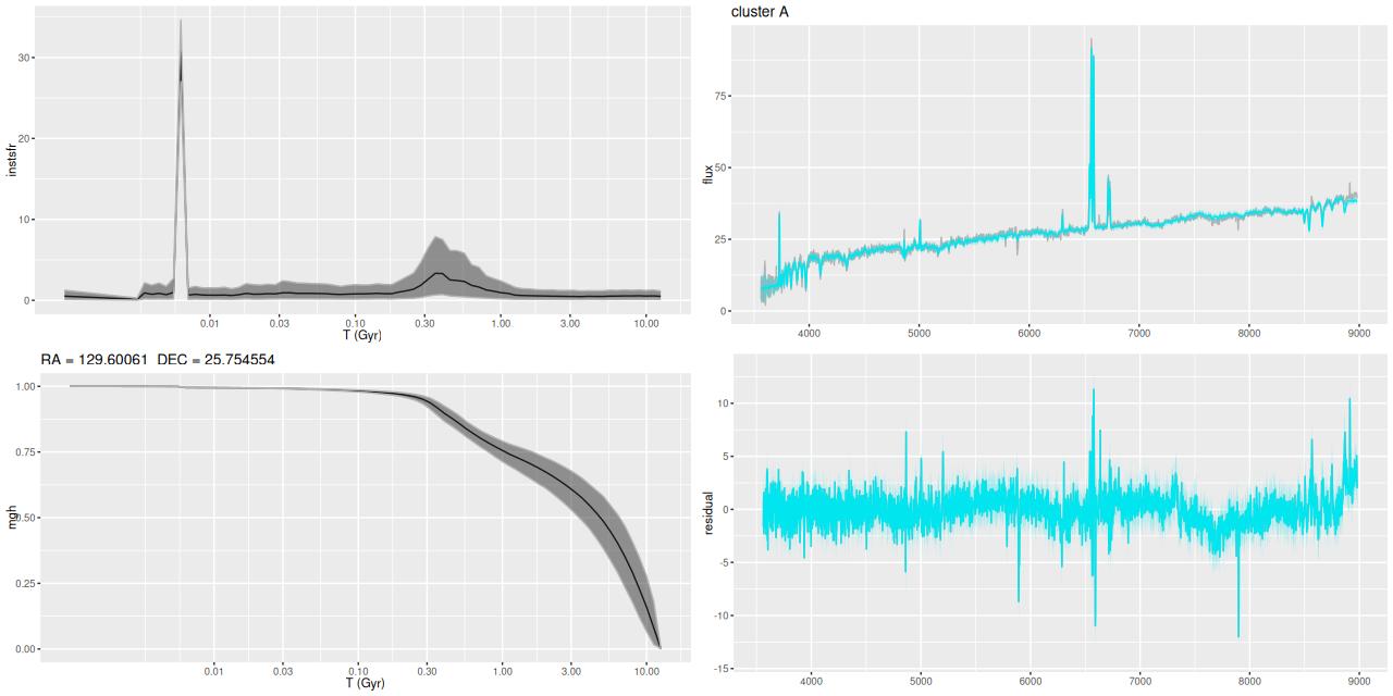
I picked four regions from the center. First is the fiber closest to the nucleus. One oddity of the RSS files is the central fiber is usually offset from the IFU center, in this case by about 3/4″ to the NW. The IFU center is exactly at the consensus position of the nucleus, and there are two fibers that straddle it. The other one is located just to the SE– notice that it has a much higher peak star formation rate than its immediate neighbor and a considerably redder continuum. The region with the highest 100 Myr average star formation rate is the neighbor to the NE, which is close to the cluster aggregation “B” in the HST image at the top of this post. Finally for the center spectra, the highest 10 Myr averaged SFR density of ≈7 M☉/yr/kpc2 is the region to the east that is centered in a prominent dust lane and includes at least part of cluster complex “A”. It also has the highest model stellar attenuation (τV≈3.3) and the highest Hα luminosity density corrected for stellar attenuation.
Fits to the data are somewhat problematic in the center. The non-Gaussian emission line profiles are prominent in the residuals. and there are systematic residuals in the stellar continuum as well. The complex dust geometry and kinematic decoupling of gas and stars are likely contributors to the lack of fit, and there are the usual issues of possibly missing ingredients in the inputs. How much the fit errors affect the SFH models is unknown.
NGC 2623 (MaNGA plateifu 9507-12704) – Sample star formation histories and posterior predictive fits to the spectra. Fiber center position and galaxy region are indicated on left and right panels respectively
A brief comparison with Cortijo-Ferrero
As I mentioned previously Cortijo-Ferrero (2017a, 2017b) published two papers studying this galaxy and a small number of other (U)LIRGS using data from CALIFA and a few other instruments. Their objectives in paper (a) were essentially the same as mine in these posts, and their methods were somewhat similar. For spectral fitting they used a code named STARLIGHT, which is not Bayesian and as far as I can tell doesn’t have any convergence guarantees but does perform nonparametric SFH modeling.
The first paper devotes one section apiece to ionized gas properties and stellar populations. Since I’ve discussed the former at some length in my previous posts I won’t review their results in detail. Quantities that I was able to compare agree well. They also found the kinematic center of the gas to be offset 2″ to the east of the nucleus, in agreement with my results and Lipari. They comment that the offset is “within (their) spatial resolution,” which is true but misses the point that the entire rotating structure is much larger and is clearly offset from the nucleus even on visual inspection.
For comparison purposes I’m going to reproduce some of their graphical results. They have maps of many quantities as well but visual comparisons are difficult because they are displayed at postage stamp size in the online journal papers and also because the authors made some truly atrocious choices of color palettes. I’ve already displayed a map of stellar mass surface density and its trend with radius, which can be compared to their figure 4 in paper (a). The values and trends with radius are similar in my models to theirs although I don’t see a break in the relation as shown in their lower plot.
Their model for stellar dust attenuation is similar to mine: they assume a single foreground screen with Calzetti attenuation. I include an additional parameter controlling the overall steepness of the attenuation curve, which essentially amounts to allowing RV to be variable. The peak values near the center are considerably higher in my models than theirs (cf figure 5 in paper a). This could be partly due to the slightly higher spatial resolution in MaNGA. More importantly perhaps my models have a “greyer” attenuation curve than Calzetti’s in the center which means a larger attenuation value is required for a given amount of reddening. Farther out there is good agreement.
NGC 2623 (MaNGA plateifu 9507-12704) – Stellar attenuation τV vs. radius in half light radii
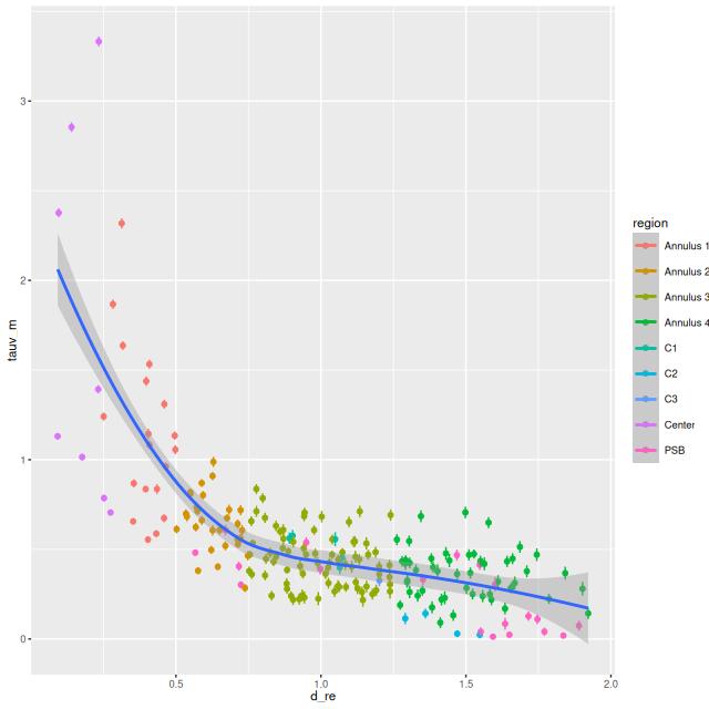
As a bit of an aside, my standard postprocessing includes estimates of dust attenuation of ionized gas using the Balmer decrement method with an assumed intrinsic ratio of Hα/Hβ = 2.86. Keeping only spectra with 3σ detections in both I get the following relation between gas and stellar attenuation. The slope of the straight line from a simple linear regression is 1.74 ± 0.06 (1 σ), which is consistent with their results (section 4.3) and, I think, other literature sources.
NGC 2623 (MaNGA plateifu 9507-12704) – Ionized gas τV vs. stellar τV for regions with detections in both Hα and Hβ
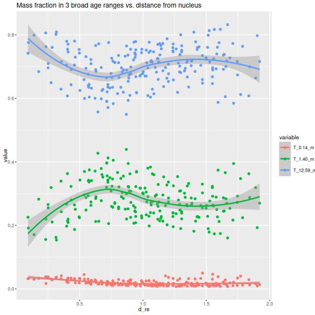
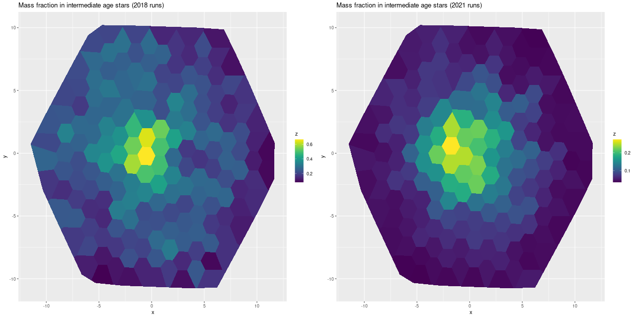
For reasons that escape me in paper (a) they chose to examine stellar population ages in 3 broad ranges: young (t ≤ 140 Myr), intermediate (140 Myr < t ≤ 1.4 Gyr), and old (t > 1.4 Gyr). I have a routine to calculate mass fractions in arbitrary age ranges, so I reproduce their figure 8:
NGC 2623 (MaNGA plateifu 9507-12704) – radial distribution of mass fraction in “young”, “intermediate,” and “old” populations
In contrast to their result there is no location where there is as much mass in “intermediate” age stars as “old” ones. However, and in agreement with them, if the SFR were constant over cosmic history there should only be about 10-11% of the total mass in young and intermediate age stars, suggesting an enhancement in SFR of a factor of ~2-3 over the past ~Gyr.
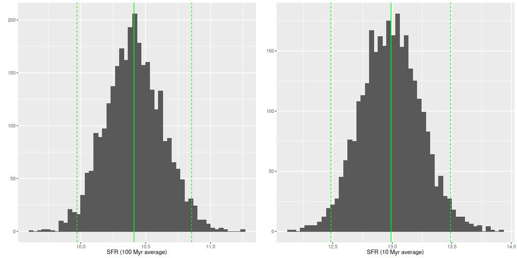
I calculated the total (IFU wide) star formation rate by summing over all individual models. The histograms below are for 100 and 10 Myr time spans: the estimated SFR has actually increased, from ≈ 10.4 M☉/yr to 13 M☉/yr in the last 10 Myr, with nominal uncertainties of ±0.5. This is entirely driven by a recent increase in the near-nuclear SFR.
NGC 2623 (MaNGA plateifu 9507-12704) – model total star formation rate on 100 and 10 Myr time intervals
SFR estimates based on infrared data tend, understandably, to be higher — the literature sources I noted at the top gave estimates of 40-70 M☉/yr. Cortijo-Ferrero give estimates of ~8-12 M☉/yr depending on time span considered.
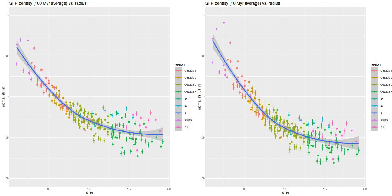
Paper (b) chose a different set of age ranges to focus on: 30, 300, and 1000 Myr, although they only discussed 300 Myr averaged star formation briefly. Instead of trying to reproduce their results for those SF timescales I’ll just show SFR density vs. radius for the 100 and 10 Myr lookback times that I’ve examined in this post. These can be compared to their figures 5 and 6. My 10 Myr plot for SFR density2add 3 to the log SFR density values to convert to the same units. looks similar to their 30 Myr except the peak values in the center are higher. In my models this is because the center has just turned on in the last <10 Myr.
NGC 2623 (MaNGA plateifu 9507-12704) – SFR density vs. radius/half light radius, 100 and 10 Myr time intervals
My sSFR plots don’t resemble theirs (figure 6) very closely. Both have a negative gradient within 1 half light radius while theirs have very shallow gradients. The steeper gradient in the 10 Myr plot is due to the recent central starburst and the slow decline of star formation outside the central few kpc.
NGC 2623 (MaNGA plateifu 9507-12704) – Specific star formation rate vs. radius in 100 and 10 Myr time interval. Units are yr-1, logarithmically scaled.
Looking back at the SFH plots by region, there appear to be 3 epochs of accelerated star formation. The oldest begins at ~1 Gyr, the second at ~300 Myr, and finally there is a central starburst with age ≲10 Myr. Privon’s merger simulation, which is the only source for this system, places the first pericenter passage at ~220 Myr lookback time Without knowing what level of accuracy to expect from this kind of simulation this appears to be excellent agreement, so we can confidently associate the “pie wedge” with this event, as well as the enhancement in SFR at about the same age in the very center.
What’s more puzzling is the apparent increase in SFR long before the final stages of the merger. In most recent high resolution simulations that I’ve seen SFR increases above baseline only shortly before first pericenter passage (e.g. Renaud et al. 2014).
Slightly puzzling also is that if coalescence occurred ~85 Myr ago as in Privon’s simulation there is no trace of its effect in my models. The current central starburst must have been delayed considerably compared to the predicted almost immediate starburst in recent simulations.
This is one of about 10% of candidate PSBs in the Leung et al. sample that was rejected for further analysis based on fitting issues. Oddly, this was classified as a Central PSB, which is clearly wrong (and which a cursory literature search would confirm). Their fitting issues may have arisen from their strategy of binning all spectra meeting their PSB criteria into a single one. This can’t work when physical conditions, particularly dust attenuation, vary rapidly.
I have recently, after several months of leisurely computing, completed model runs for all 91 data sets in this sample. A detailed analysis is some ways off. I need to go through each model run — some had very poor fits, possible calibration errors, or low S/N data.
I’m going to continue my discussion of the models for the MaNGA observation of NGC 2623 (aka Arp 243, etc.) in MaNGA plateifu 9507-12704 (mangaid 1-605367). First I’ll look at emission lines and line ratios. I don’t have any fresh insights to offer, but it’s useful for me at least to compare to earlier IFU based studies by Lipari et al. (2004) and Cortijo-Ferrero et al. (2017).
Next I’ll turn to stellar populations and star formation histories. This will prove to be quite interesting: there are several distinct regions in different evolutionary states. That will be in my next post.
Emission line properties
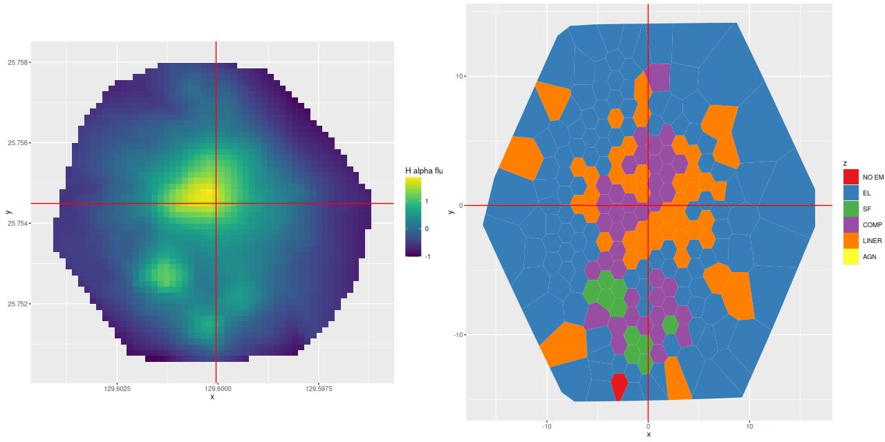
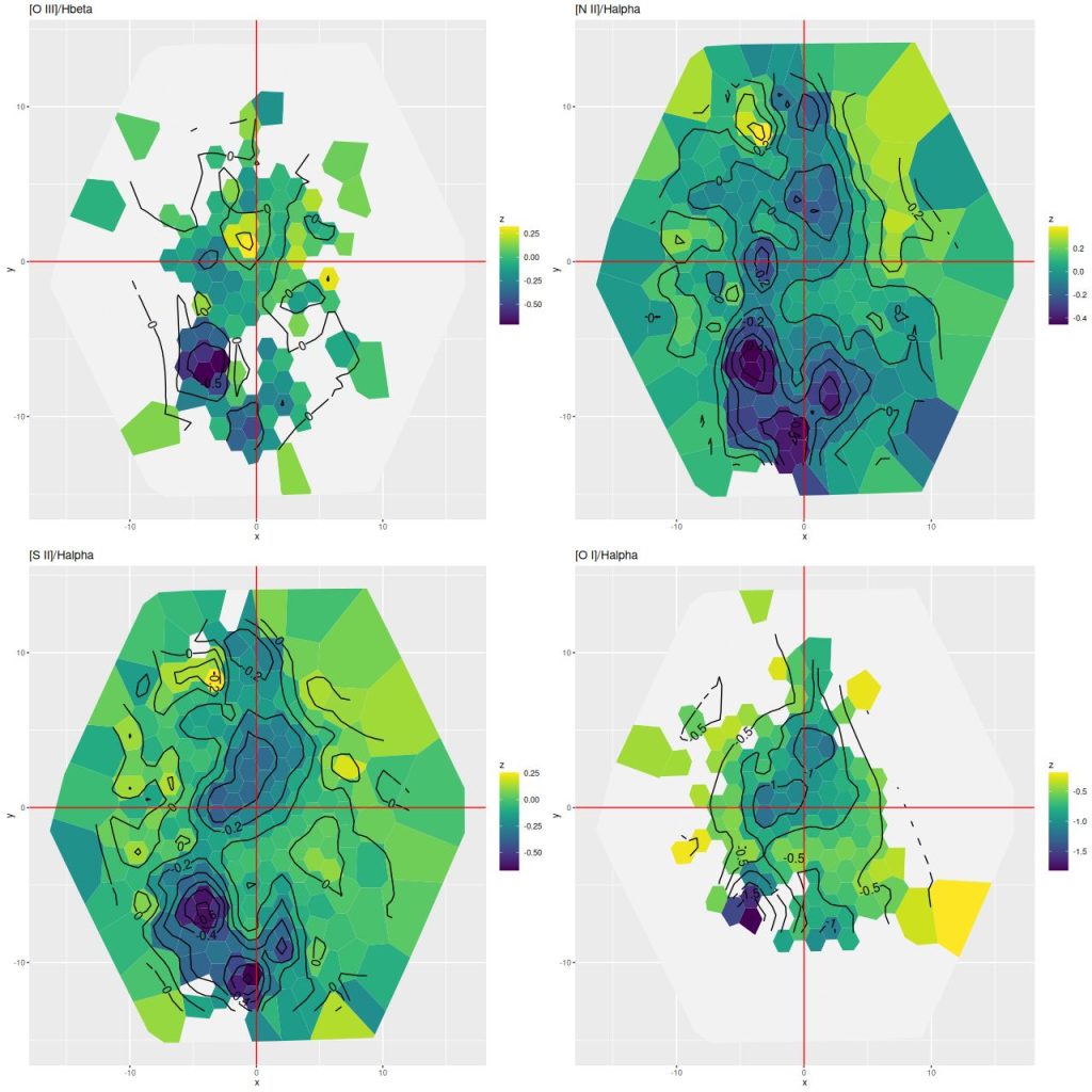
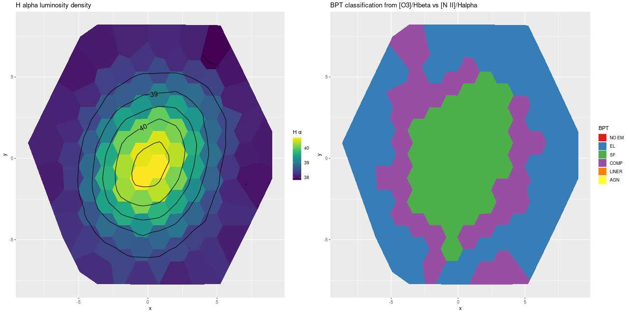
For an overview the plot below maps the Hα flux density1I think I made a factor of 4 error, but that doesn’t affect relative values and hence the color rendering. uncorrected for attenuation. The values are logarithmically scaled. The brightest region by some margin is just NE of the nucleus, with a secondary peak a short distance to the east. The three brighter areas to the south of the nucleus are H II regions.
The right hand panel shows BPT classifications from the [O III] 5007/Hβ vs [N II] 6584/Hα diagnostic following Kauffmann (2003), augmented with a weak line class for spectra without firm detections in one or more of those lines or [O II] 3727-3729 (labelled “EL” in the graph), and another (“NO EM”) for spectra with no firm detections at all. Just over half of the spectra have too weak lines to classify, while 40% fall in the LINER or “composite” bins mostly in a connected region surrounding the nucleus. The three regions in the south have unambiguously starforming BPT classifications.
NGC 2623 (MaNGA plateifu 9507-12704) – (L) Hα flux density. (R) BPT classification from [O III]/Hβ vs [N II]/Hα per Kauffmann 2003
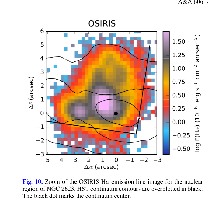
The shape and relative values of the Hα flux near the nucleus agree very well with a higher resolution map published by Cortijo-Ferrero:
Screenshot of Hα flux density from Cortijo-Ferrero et al. 2017
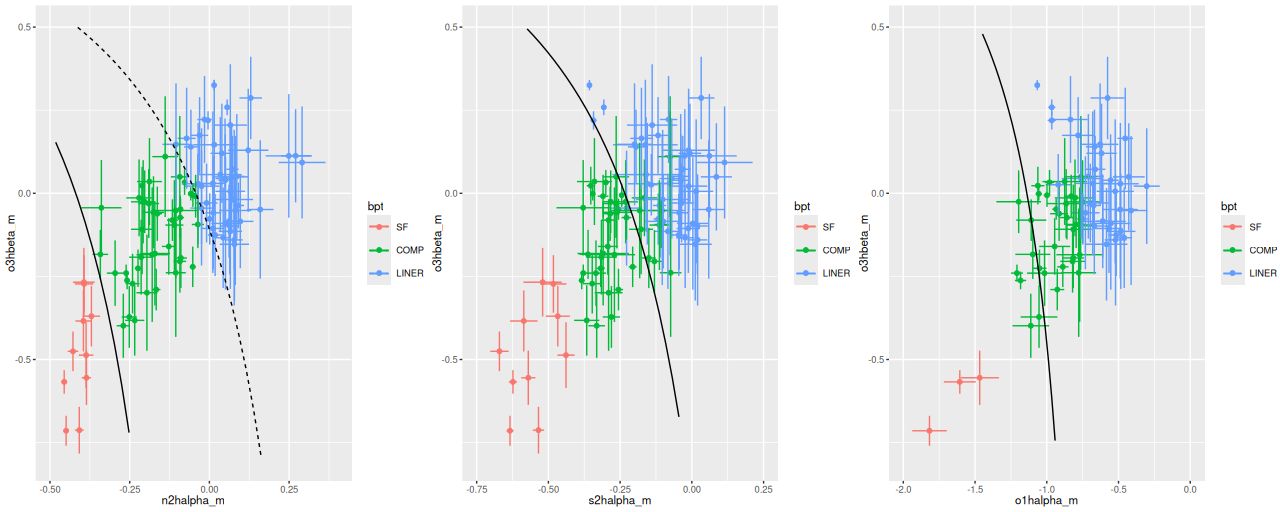
Taking a closer look I plotted line ratios for the 3 BPT diagnostics that are commonly used with SDSS data, namely [O III] 5007/Hβ vs. [N II] 6584/Hα, {S III] 6717+6730/Hα, and [O II] 6300/Hα. Only points with 3σ detections in the relevant lines are plotted. Lines marking the boundaries between star forming and something else are from Kewley et al. (2006) and Kauffmann (2003). Note that in all 3 plots the regions with star forming line ratios stay on the star forming side of the boundaries, as do the areas with LINER like ratios. The “composite” regions on the other hand are in the star forming side of the boundary in the [SII/Hα plot while many shift into the LINER region in [O I]/Hα.
NGC 2623 (MaNGA plateifu 9507-12704) – BPT diagnositcs for commonly used emission line ratios: (L) [N II]/Hα, (C) [S ii]/Hα , (R) [O I 6300]/Hα. Lines are SF/something else boundaries from Kauffmann 2003 and Kewley 2006. Only spectra with 3σ detections in the relevant lines are plotted.
There’s a fairly general consensus on the likely ionization sources. X ray observations demonstrate the existence of a heavily obscured low luminosity AGN (e.g. Yamada et al. 2021 and many others) along with a nuclear starburst. Just outside the nucleus shock excitation was proposed as the main ionizing source already by Lipari, and confirmed by Cortijo-Ferrero’s CALIFA observations, although they also emphasize the possible role of recent star formation.
Alatalo et al. (2016) commented that “[O I]/Hα is a particularly good tracer of shock excitation,” citing Rich et al. (2010) and another source. The latter is particularly interesting because they performed a detailed IFU based analysis of a galaxy (NGC 839) that, while not being involved in a merger, shows similar properties of moderately high velocity outflow probably driven by a nuclear starburst with extensive regions of post-starburst spectra. Their BPT plots look remarkably similar to mine, with most spectra in the “composite” region in the [N II]/Hα plot shifting into the LINER region in [O I]/Hα.
Maps of the line ratios are shown below: again only regions with 3σ detections in the relevant lines are shown, which considerably limits the spatial coverage of [O III]/Hβ and [O I]/Hα. A few points to note: the peak value of [O III]/Hβ is just NE of the nucleus and likely near the source driving the outflow. All of the line ratios generally increase away from the nucleus to the NW and NE. To the south the three H II regions are prominent.
NGC 2623 (MaNGA plateifu 9507-12704) – Maps of emission line ratios. (TL) [O III 5007]/Hβ (TR) [N II 6584]/Hα (BL) [S II}/Hα (BR) [O I 6300]/Hα. Only spectra with 3σ detections in the relevant lines are shown.
The main result of this analysis is it validates my approach of modeling emission line and stellar contributions simultaneously. This is uncommon but not unheard of in the spectral fitting industry2I believe Capellari’s ppxf has this capability. Since some form of stellar template is needed to get unbiased estimates of emission line properties, from my point of view it makes sense to model both at once. My results for this galaxy agree very well with the two earlier major studies.
I’m going to hit publish now and continue with stellar populations in my next post. I may actually have something new to say about them.
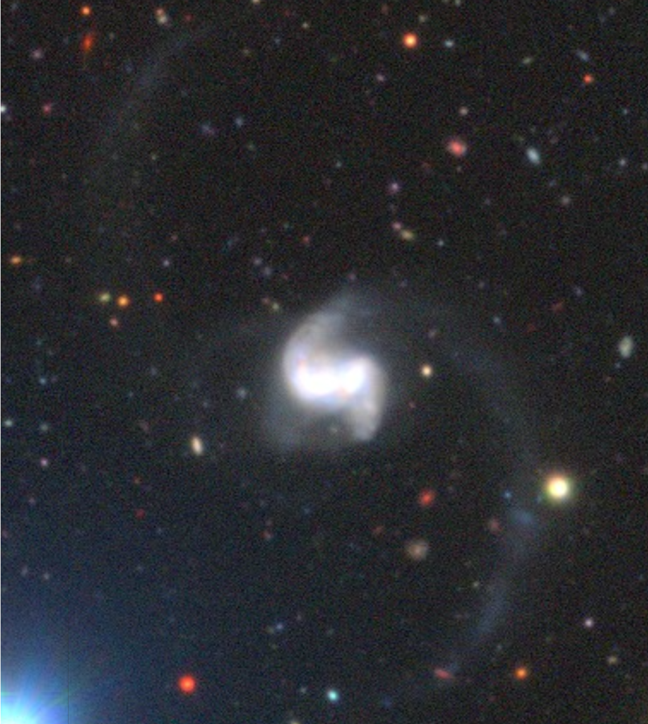
I’ve been making my way through Leung’s PSB sample and noticed this exceptionally interesting “CPSB” sample member, which oddly enough they chose not to include in their analysis. This is NGC 2623, a rather famous merging galaxy pair that was one of Toomre‘s exemplars of a late stage merger. This is a well studied system, with over 500 references listed in NED and observations apparently in every electromagnetic frequency range for which telescopes exist (nothing from JWST yet though).
MaNGA targeted it with one of their largest IFUs, which covers most of the visible light (at the depth of SDSS imaging) of the merger remnant, but very little of the tidal tails. There’s also a CALIFA IFU dataset with a larger spatial footprint but lower spectral resolution. I haven’t looked at that in detail yet except to estimate the relative velocity field..
As usual I work with RSS spectra stacked and binned to a target S/N. For this final post starburst project I’m trying to set a higher S/N threshold. In this case I ended up with 214 spectra with S/N per pixel ranging from 8.5 to 42.5.
MaNGA plateifu 9507-12704, mangaid 1-605367
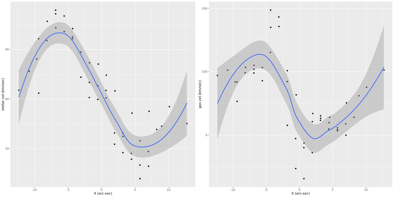
Kinematics
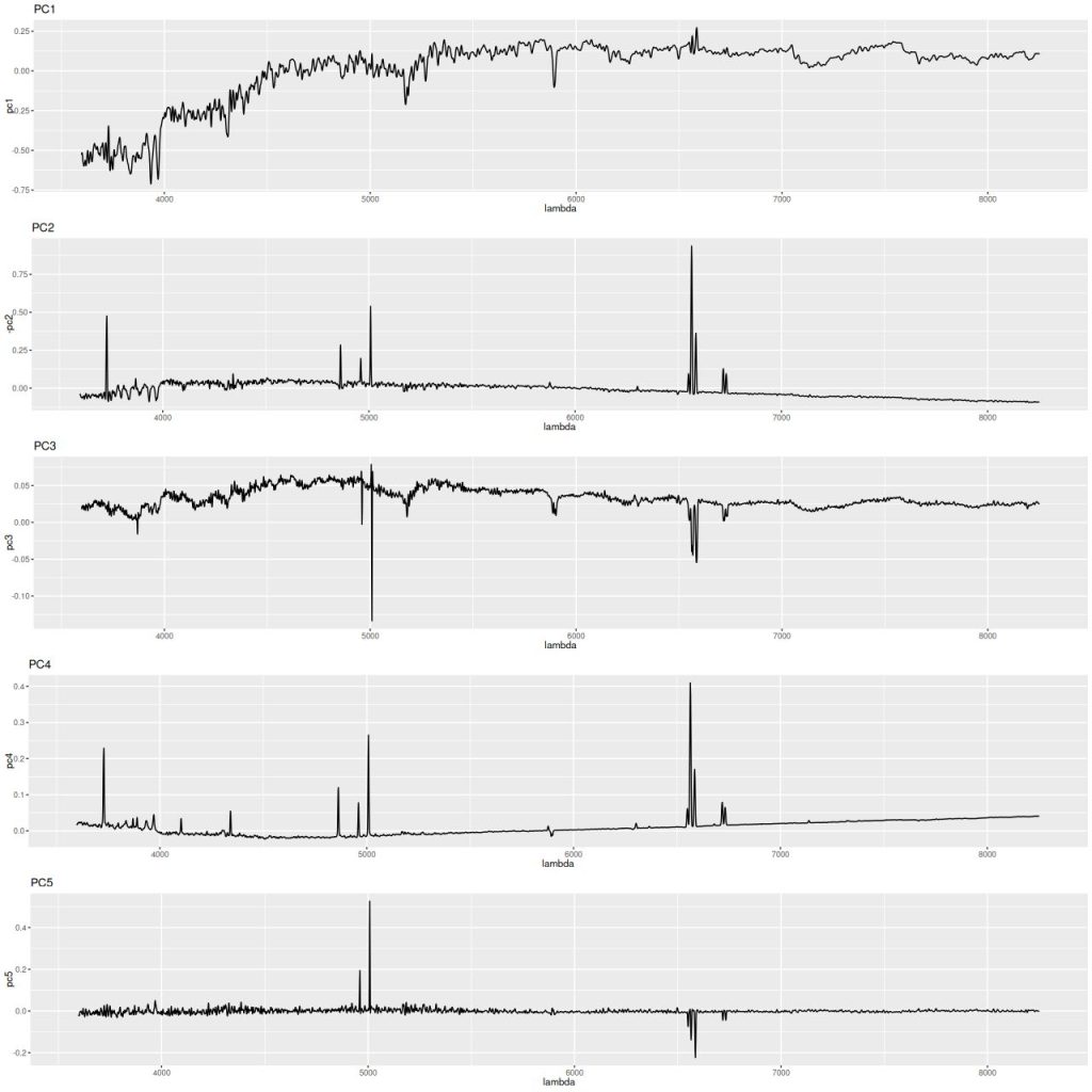
I’ll first discuss the stellar and gas kinematics, since calculating redshift offsets is the first thing I do after loading data and binning to a target S/N. I use a straightforward template matching procedure using as templates a set of 15 eigenspectra that I computed some years ago using an algorithm published by Blanton and Roweis (2007) and a fairly large sample of SDSS galaxy spectra. The first 5 are shown below. The first two look like real spectra of a passively evolving ETG and a star forming galaxy respectively. The rest represent departures from these archetypes. I did not mask emission lines, so both absorption and emission lines are present, often with the opposite of expected signs.
First 5 eigenspectra used as templates for calculating redshift offsets
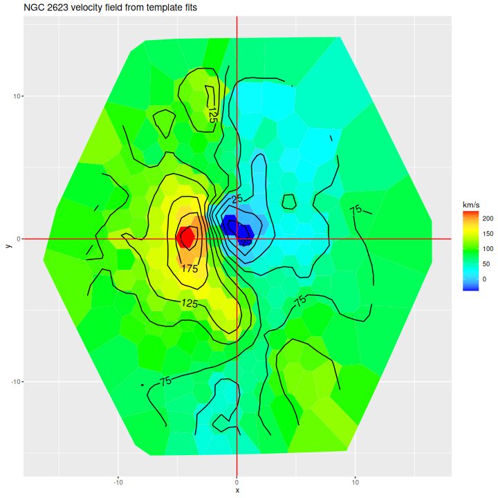
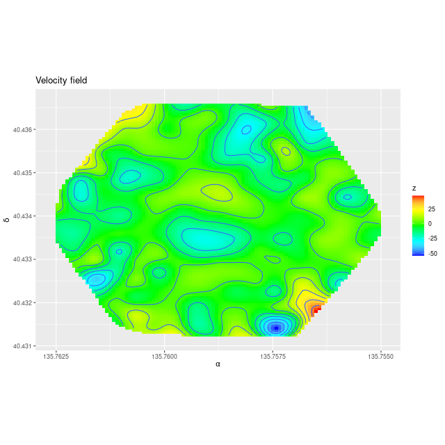
Here is the computed velocity field (converted from redshift offsets from the published system redshift of z=0.01818). As I’ve said before and is obviously the case from the plot above the template fitting procedure gives a blended velocity estimate that in any given spectrum might be dominated by emission, absorption, or a combination. In this case it turns out that emission lines dominate in the IFU center, with the outer parts dominated by stellar motion.
NGC 2623 (MaNGA plateifu 9507-12704) velocity field from template fit
I often check Marvin to compare MaNGA data analysis pipeline measurements to mine. Sometimes visual comparisons are hampered by unfortunate choices of color palettes by the Marvin team. That’s especially the case for velocities where they use shades of red, white, and blue to represent positive, ~ 0, and negative velocities. It was apparent though that the stars and gas are kinematically decoupled at least in the center.
To investigate further I decided to dust off my old code for non-parametric line of sight velocity distribution modeling1which I last wrote about here and several previous posts., made some small modifications, and ran on the same 214 binned spectra. The results for the mean velocity offsets from the system redshift are shown below for stars (L) and gas (R). For easier comparison to Marvin I interpolated the model outputs to 0.5″ x 0.5″ pixels.
Even though people who claim to know generally disapprove of the use of rainbows in graphics I like to use them for velocity maps. In this case though using a more perceptually uniform palette (viridis with 256 levels) reveals some interesting details that aren’t as evident with a rainbow palette.
NGC 2623 (MaNGA plateifu 9507-12704) Estimated stellar and ionized gas velocity distributions.
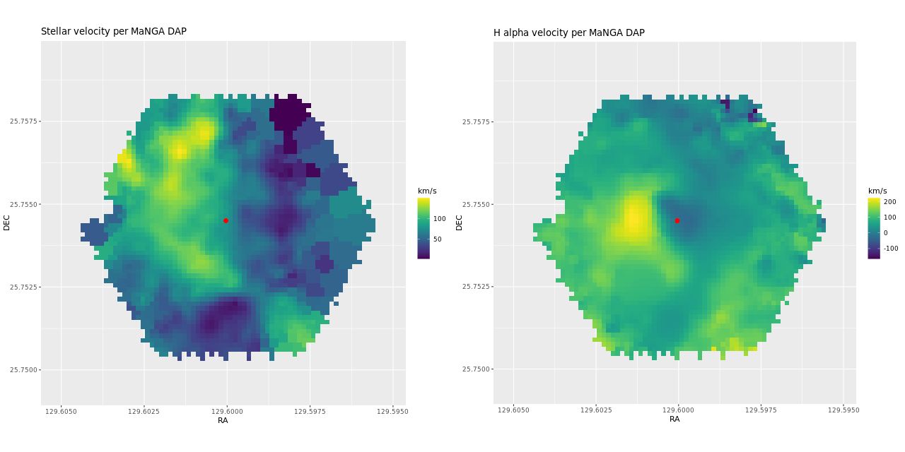
I also downloaded the maps from Skyserver that are displayed in Marvin. Below are the stellar and Hα velocity plots2[N II] 6584 might have been a better choice since it’s brighter than Hα over most of the galaxy.. I haven’t tried a detailed quantitative comparison because it’s not easy to properly register the maps, but it’s evident that these are very similar.
NGC 2623 (MaNGA plateifu 9507-12704) Estimated stellar and ionized gas velocity distributions from MaNGA DAP.
The velocity maps have several interesting features. First, the ionized gas is rapidly rotating within the inner ~2 kpc, but there’s no apparent organized rotation farther out. Zooming in on the center the rotation axis appears to be offset to the east of the IFU center (marked), which is exactly at the position of the nucleus, by ≈ 1.6″ (800 pc) if the unlabelled 75 km/sec contour line is taken as the axis of rotation. In a very thorough analysis of IFU data that preceded MaNGA by more than a decade Lipari et al. (2004) also noted a displacement of the kinematic center of 1.1″ to the east of the nucleus — in good agreement with my estimate given the limited resolution of MaNGA data. There also appears to be good qualitative agreement on gas velocities in the area with overlapping observations, which is roughly the zoomed in region below (see their figure 8a). NGC 2623 was also observed in the CALIFA survey, and its kinematics are discussed in Barrera-Ballesteros et al. (2015). Their velocity fields appear broadly similar, but visual comparison is hampered by the small size of their figures.
Outside the nuclear region gas and stellar velocities are more nearly equal although with some scatter that may simply be due to measurement errors.
A minor point that’s maybe worth noting is the overall mean velocity in both the stellar and gas measurements is ≈70 km/sec, which suggests the system redshift of z = 0.01818 adopted by MaNGA is low by ≈2×10⁻⁴, or z = 0.01842 (cz = 5522 km/sec). This is close to the fiducial heliocentric redshift of 0.01851 adopted by NED and well within the range of values listed there.
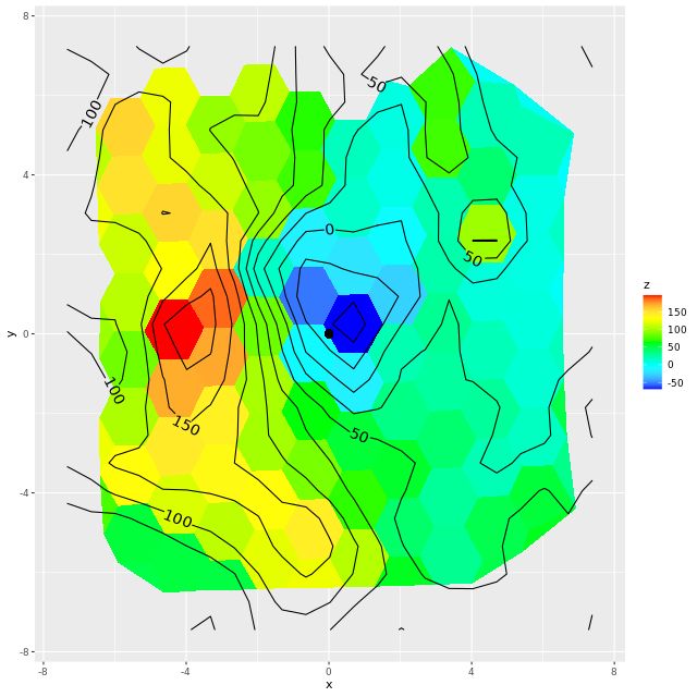
Two features I find really interesting that are especially prominent in the stellar velocity map are a pair of long, irregular, but mostly connected arcs that stretch across the full width of the IFU. One arc is relatively redshifted, exiting (entering?) the IFU at the position of the small portion of the SW tidal tail that’s within the footprint, appears to cross the other arc, then stretches to the south and east of the nuclear region, terminating to the north approximately where the northern tidal tail enters the IFU footprint. The other, relatively blue shifted arc starts in the south in the area of the blue, wedge shaped region (which I will discuss much more later), curves around to the west of the nuclear region, and appears to terminate somewhere in the NW region of the IFU.
To date there is only one N-body simulation of the NGC 2623 merger, by Privon et al. (2013). In their model the blue wedge in the south is material from the progenitor that formed the northern tidal tail, has passed through the main body and is now falling back in. In their simulations there are regions even in the main body of the merger remnant where the progenitors aren’t well mixed. I’m wondering if these apparently connected regions with systematic velocity offsets might reflect that lack of complete mixing, with the blue shifted regions falling into the galaxy from behind and the redshifted falling from above.
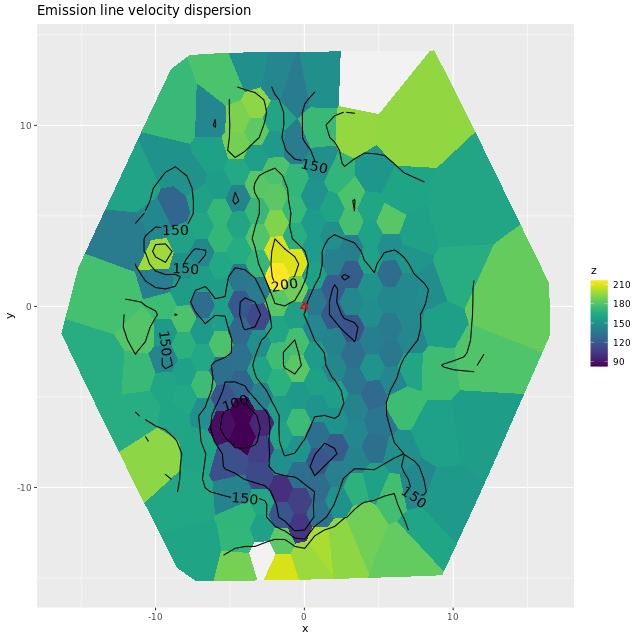
One final plot for now: the average emission line velocity dispersion. These are “raw” values uncorrected for spectral resolution. The relatively high values to the NE of the nucleus might be associated with the outflow discovered by Lipari et al. The low values well south of the nucleus are from H II regions.
NGC 2623 (MaNGA plateifu 9507-12704) mean Ionized gas velocity dispersion
This post turned out longer and took longer to write than I expected, so I will break it up into two or perhaps more. Next time I’ll look at some other physical properties and perhaps model star formation histories.
Update
Barrera-Ballesteros found regular stellar rotation out to the maximum radius of 6″ (2.2 kpc) that they had usable data. Both they and Lipari found a sinusoidal rotation curve for the ionized gas. I was skeptical of the claimed large scale stellar rotation since visual inspection of the velocity maps didn’t show an obvious velocity gradient in any direction. But, I decided to take a closer look anyway. Since the kinematic position angle for both is close enough to 90o I just plotted velocities for bins within ±2″ of the horizontal axis. The results are plotted separately for stars (L) and gas (R). The curved lines with “confidence bands” are loess fits to the plotted data and should absolutely not be taken seriously as a model of the rotation curves. It’s notable though that if’s fairly symmetrical for the stellar velocities and if the true system velocity is 70 km/sec larger than adopted by MaNGA its kinematic center is right at the IFU center. The ionized gas kinematic center is clearly seen as offset to the east, as noted above.
NGC 2623 (MaNGA plateifu 9507-12704) – Stellar and gas velocities within 2″ of the X axis
One simple way to quantify the burstiness of star formation is just to estimate the average star formation rate over large time intervals divided by the average SFR over cosmic time. Of particular interest is the time interval between ~100 Myr and ~1 Gyr since this is roughly the time interval that a post-starburst galaxy is recognizable as such.
Partly because it happens to still be in my active workspace and partly because it’s really interesting I’m going to take another look at SDSS J095343.89-000524.7 (MaNGA mangaid 1-897). This was in the post-starburst ancillary sample, selected from the catalog by Pattarakijwanich et al.
This image from the Subaru HSC-SSP survey1retrieved as a screenshot from the Legacy Survey sky browser. is much deeper than SDSS imaging and clearly shows extended tidal tails and debris, suggesting that these galaxies have been interacting for some time.
SDSS J095343.89-000524.7 (observed as mangaid 1-897).
Image screenshot from Subaru HSC survey.
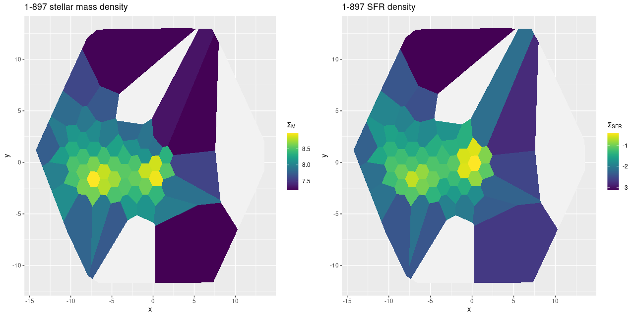
Moving on to various properties derived from the MaNGA spectroscopy and my SFH models with, still, EMILES based SSP models. First here are maps of stellar mass density and 100 Myr averaged star formation rate density. Note that I rebinned the spectra from two posts ago to try to capture more of the tidal tails while excluding the truly blank regions of sky. There are two clear peaks in the stellar mass density separated by a projected distance of about 11 kpc. The central stellar mass densities are nearly the same at about 108.95 M☉/kpc2 . Interestingly enough the bright white peak in surface brightness appears not to coincide with the western peak in stellar mass density, but is offset by a small amount to the north.
Note also that the highest recent star formation is offset to the north of the apparent western nucleus. I’ll look at that in more detail below.
MaNGA plateifu 10843-9101 (mangaid 1-897). Maps of stellar mass density and star formation rate density.
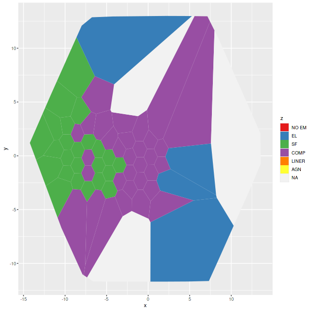
The ionized gas properties are rather different in the two galaxies. Below are BPT classifications using, as usual for me, just the [O III]/Hβ vs. [N II]/Hα diagnostics and Kauffmann’s classification scheme. Emission line fluxes are generally stronger in the eastern galaxy with mostly star forming line ratios. Note two spectra with “composite” line ratios are near the eastern nucleus and might therefore actually be due to a mix of stellar and AGN ionization.
MaNGA plateifu 10843-9101 (mangaid 1-897). BPT classifications from [O III]/Hβ vs. [N II]/Hα diagnostics
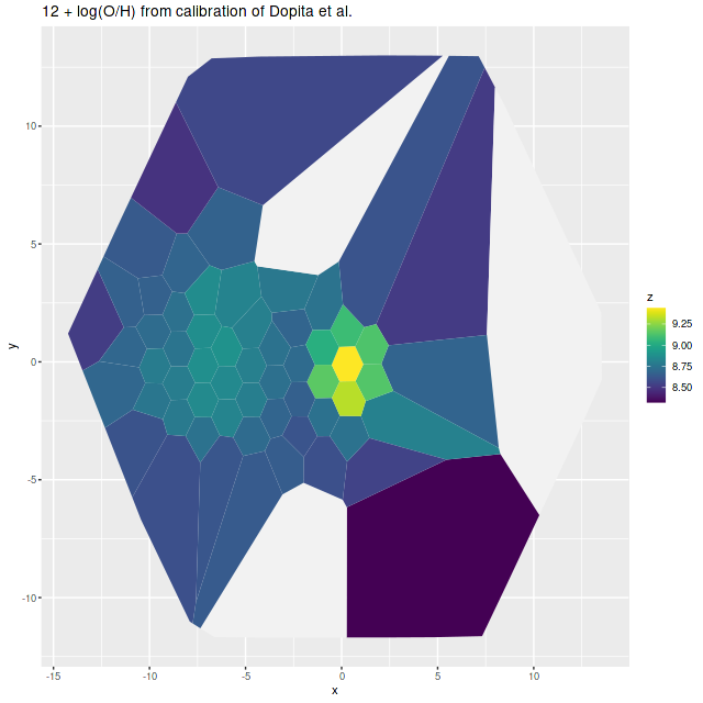
I calculate a few “strong line” gas metallicity estimates from standard literature sources. The one that seems to produce the most consistent estimates is the calibration of Dopita et al. (2016) based on the ratios of [N II 6548]/[S II 6717, 6731] and [N II]/Hα. The eastern galaxy shows a fairly smooth radial gradient while the west is considerably metal enriched in the region with the strongest starburst. The highest metallicity is right at the center of the IFU at the position of the bright white source.
MaNGA mangaid 1-897 (plateifu 10843-9101). Gas phase metallicity 12 + log(O/H) from strong line calibration of Dopita et al. (2016).
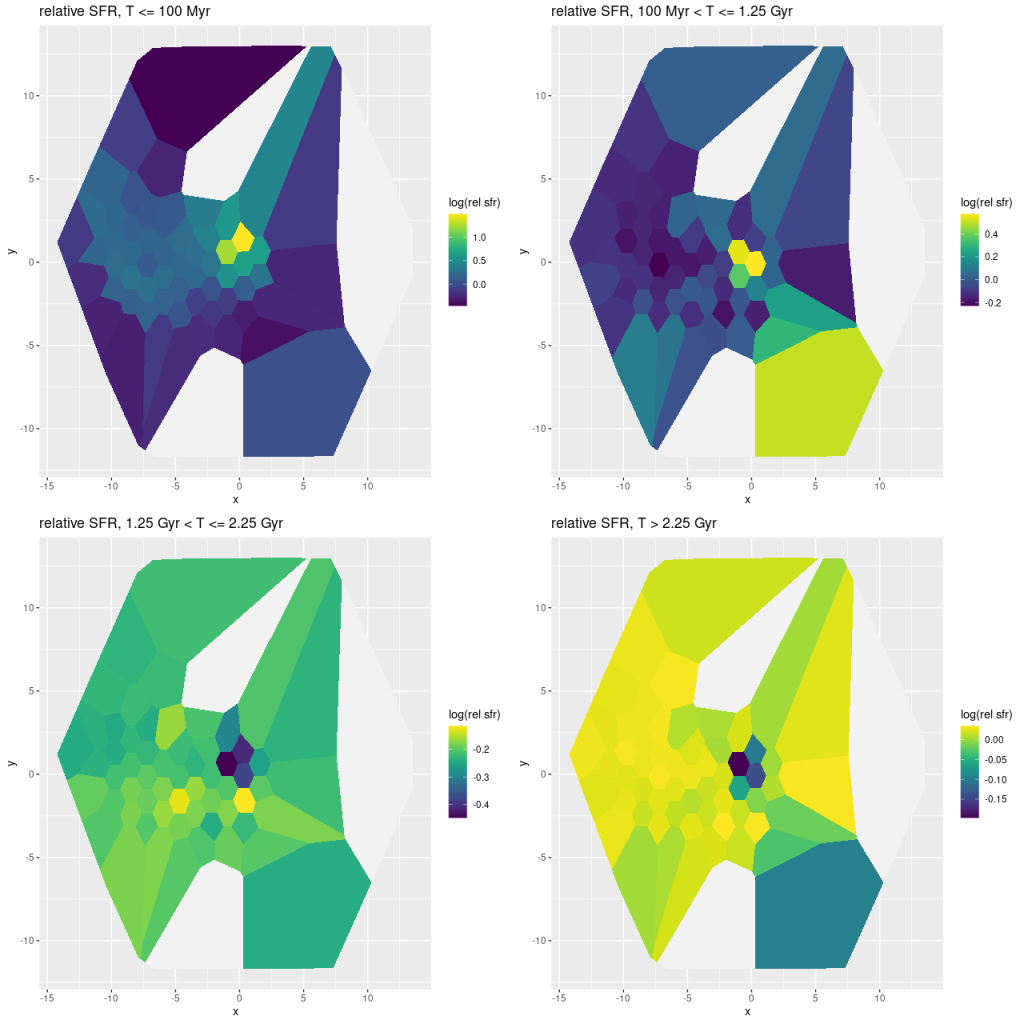
Let’s return to the idea I had at the top of the post to look at star formation rates in broad time intervals relative to the mean star formation rate over cosmic time. For this exploratory exercise I used just 4 bins with upper age limits of 0.1, 1.25, 2.25, and (nominally) 14 Gyr. There seems no point being too fastidious about calculating the bin widths: I just used the difference in nominal ages between the endpoints. I did take into account the lookback time to the galaxy, which for this one is about 1 Gyr (z = 0.083), so the final bin has a calculated width of 10.5Gyr. I chose to make the 3rd, intermediate age bin a rather short 1 Gyr wide to look for aging starbursts that might be missed using the typical selection criterion of strong Balmer absorption. In this case there’s no evidence of that: both galaxies seem to have had uneventful histories up until ~1 Gyr ago.
The top row of the plot below is the most interesting: there appear to have been two major bursts of recent star formation, both highly localized to the central region of the western galaxy. If the model estimate of the location of the peak stellar mass density is correct the fiber with the largest star formation excess in the 100 Myr – 1.25Gyr interval is offset just to the north and coincident with the IFU center. The more recent burst is also offset from the older one. There is a hint of recent accelerated star formation over most of both galaxies.
MaNGA plateifu 10843-9101 (mangaid 1-897). Maps of relative average SFR over the designated time intervals.
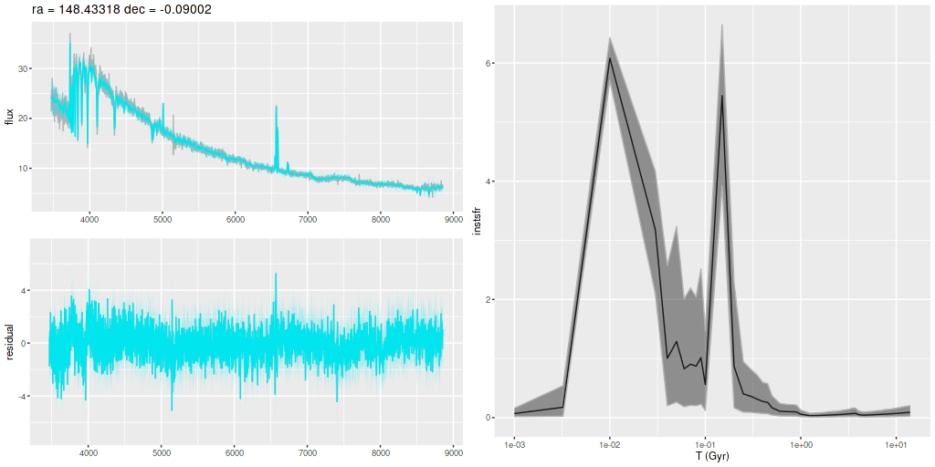
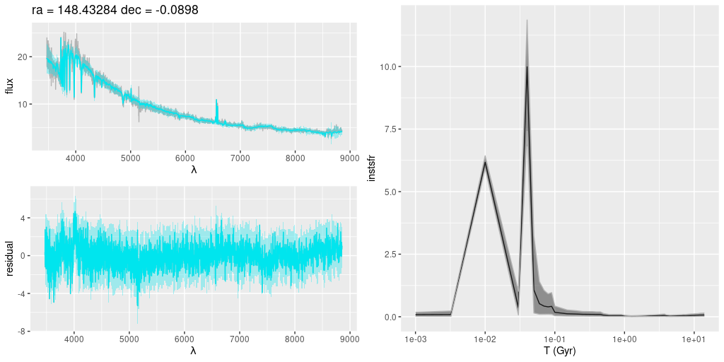
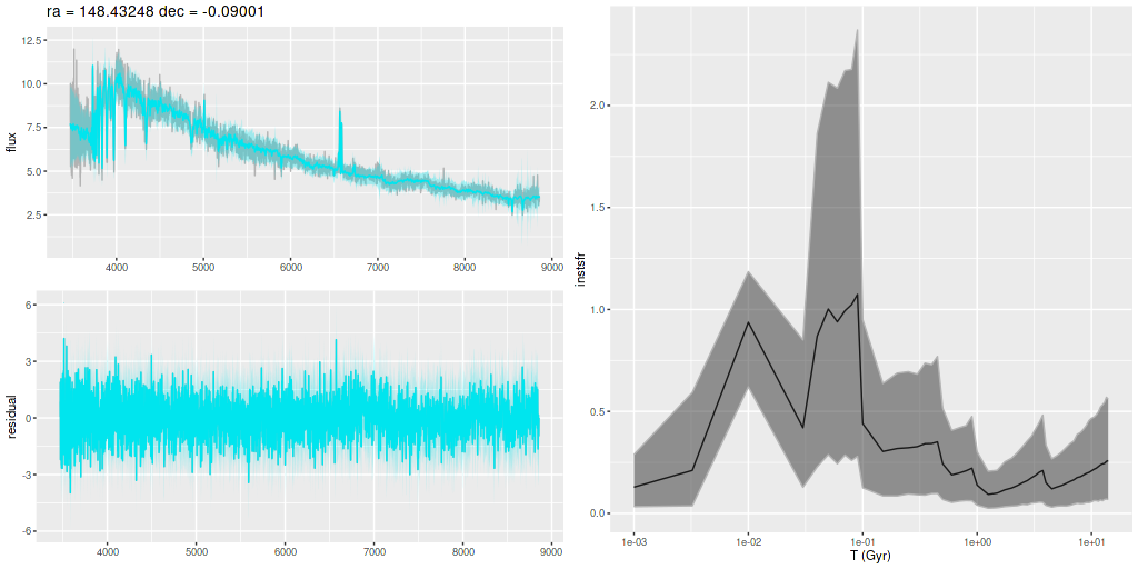
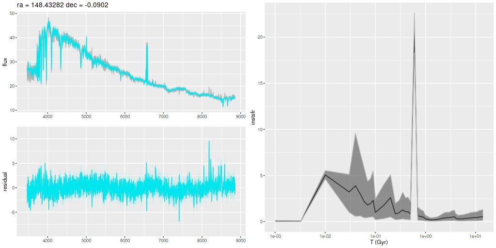
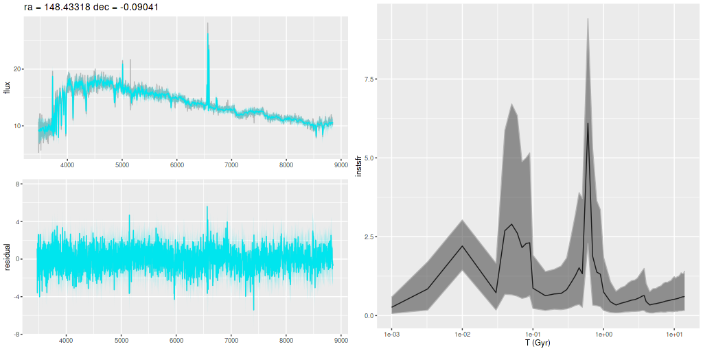
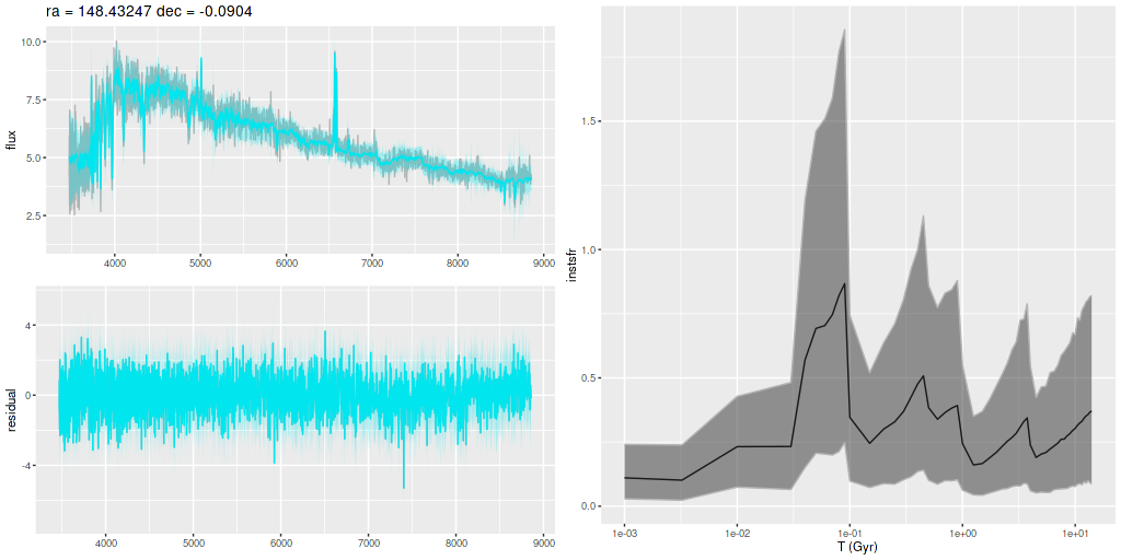
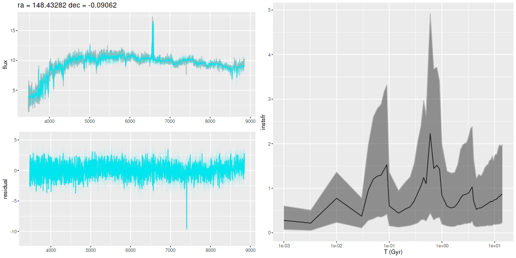
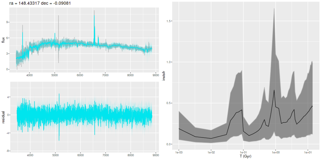
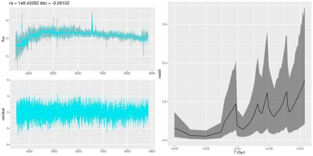
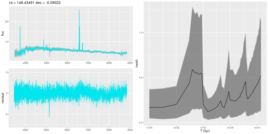
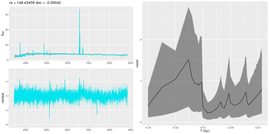
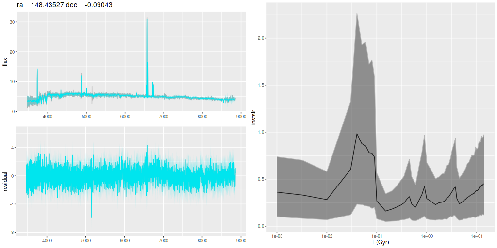
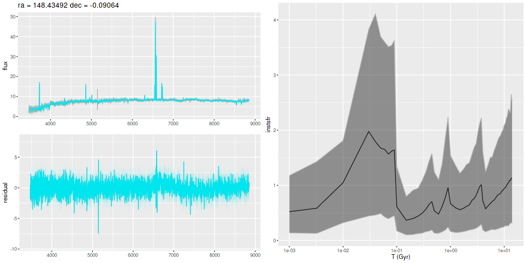
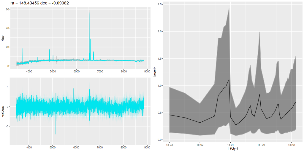
For the rest of this post I plot model fits to the spectra and star formation histories for the fibers surrounding the two nuclei. These are ordered approximately from north to south and west to east. For reference the IFU center is at (ra, dec) = (148.43291, -0.09018). The model has the peak stellar mass density in the western system at (ra, dec) = (148.4328, -0.09062). The eastern galaxy’s nucleus is at (ra, dec) = (148.4349, -0.09064).
Note below that the plots have different vertical scales. The horizontal scales are the same for both spectra and star formation histories, but at least one SFH plot is slightly misaligned.
Central region – western galaxy
MaNGA mangaid 1-897 — central region of western galaxy – spectra with fits and model star formation histories
Central region – eastern galaxy
MaNGA mangaid 1-897 — central region of eastern galaxy – spectra with fits and model star formation histories
In an earller post I mentioned a MaNGA related paper by Cheng et al. who found nearly 500 systems with post-starburst characteristics that fell in 3 broad categories: centrally concentrated PSB regions, ring-like, and irregularly located. Clearly any galaxy that was selected based on SDSS spectroscopy that’s not a false positive will have a central PSB region, although that of course doesn’t preclude extended post-starburst conditions. This particular galaxy appears to have a remarkably compact post-starburst region.
When time permits again I plan to look at the remaining 40 galaxies in this sample. Unfortunately the larger sample of Cheng et al. appears to have no published catalog.
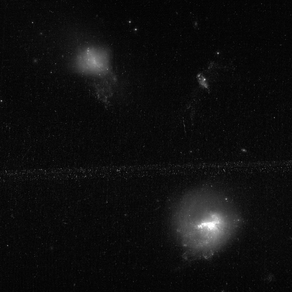
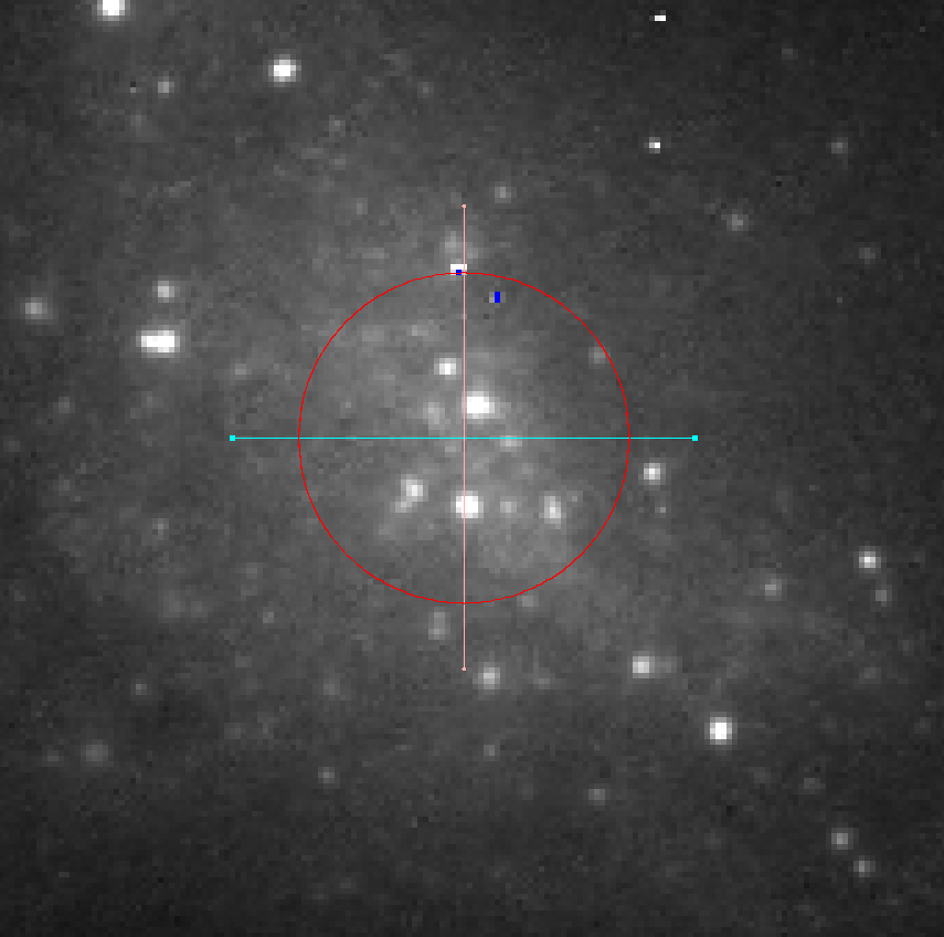
The Hubble Space Telescope “gap filler” program “Gems of the Galaxy Zoos” (proposal ID 15445, PI William Keel) had several prospective targets that I played a small role in selecting, and this recent HST observation was one of them. The actual target was the small disturbed galaxy at top left, which I will refer to as MCG +07-33-040. I don’t know if it was fortuitous that the larger and brighter UGC 10200 was also imaged in the same ACS field, but these are clearly interacting or at least have in the recent past, as is the small system in the upper right, which is identified as a blue compact galaxy with redshift z=0.00556 in Pustilnik et al. (1999). I’m going to focus on the top left galaxy in this post.
Galaxies UGC 10200 (lower right) and MCG +07-33-040 (upper left). HST/ACS, F475W filter. Proposal ID 15445, PI Keel.
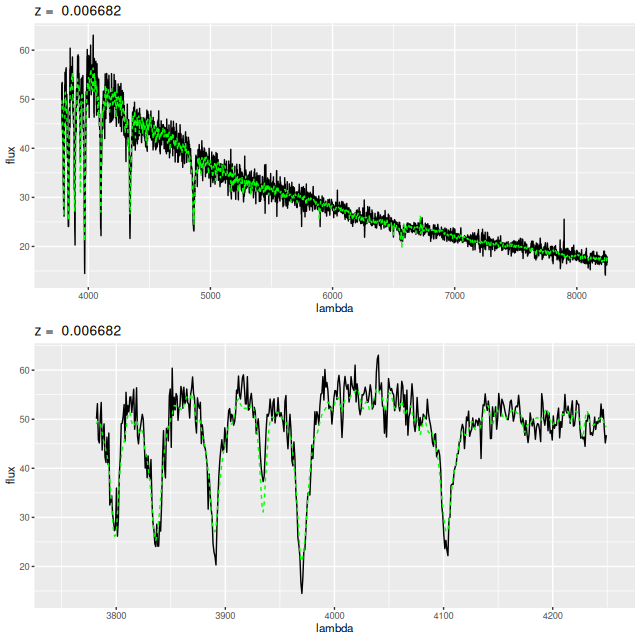
What interested me wasn’t the galaxy image so much as its SDSS spectrum, which has three interesting characteristics:
SDSS spectrum of central part of MCG +07-33-040
First, this is a classic post starburst galaxy spectrum with extremely strong Balmer absorption lines1My code measures the Lick index HδA as an exceptionally strong 8.06 ± 0.41 Å. and no obvious evidence of emission. In fact, although this designation isn’t used much anymore, it’s actually a classic “A+K” spectrum which reverses the usual “K+A” terminology to indicate the light is dominated by early type (i.e. young) stars. Second and third, the spectrum was misclassified as coming from a white dwarf star, and the redshift was erroneously estimated as around 0.004 which was the maximum allowed for stars in the SDSS data reduction pipeline. Using a variation of the code that I use to measure redshift offsets I get a robust value of z = 0.006682 ± 9E-06
Template fit to SDSS spectrum of MCG +07-33-040
This is almost exactly the same redshift as its nearby companion UGC 10200 (also in the HST image above), which has a securely determined z = 0.00664
SDSS spectrum of central region of UGC 10200
For the rest of this post I’m going to assume the Hubble flow redshift is the measured one, which with my adopted cosmological parameters2which for the record are H0 = 70 km/sec/Mpc, Ωm = 0.27, Ωλ = 0.73. make the luminosity distance 28.8 Mpc, the distance modulus m-M = 32.3 mag, and the angular scale 138 pc/” or about 7 pc per ACS pixel. The projected distance between the centers of the two bright galaxies in the HST image is about 96″ or 13.2 kpc.
I spent some time last weekend downloading and starting to learn the software Aperture Photometry Tool (APT), which is interactive software for manually performing aperture photometry. Zooming in on the center of the presumed post starburst galaxy I located the reported position of the SDSS fiber as closely as I could. In the screenshot below the aperture radius was set to 30 pixels, the same size as the SDSS spectroscopic fibers. I measured the F475W AB magnitude to be 17.90 ± 0.013 without sky subtraction, which is close enough to the SDSS g band fiberMag estimate of 18.05. The SDSS g band Petrosian magnitude estimate is 15.16, so the fiber contains about 7% of the total galaxy light.
Central region of MCG +07-33-040 with position and size of SDSS fiber overlaid. Screenshot from APT
A striking feature of the HST image is there are many point-like symmetrical objects embedded within the otherwise nearly featureless diffuse light of the galaxy. Within the SDSS fiber footprint I count about 8-10 of these (the range being due to some uncertainty about what to call point-like and symmetrical). In order to get a handle on their contribution to the spectrum I did aperture photometry on them using a 3 pixel radius aperture with median sky subtraction from a 5 to 8 pixel radius annulus. The apparent magnitudes of the 5 brightest objects range from about 22.6 to 23.1. The summed luminosity of those 5 amounts to only 3.5% of the total light in the fiber, so the spectrum is mostly telling us something about the diffuse starlight. Even if one or more of those objects are foreground stars they can’t be a significant source of contamination. Clicking around the blank regions of the HST field I found fewer than one star per SDSS fiber size region, so it’s likely there are few if any foreground stars within the visible extent of the galaxy.
There is plenty of observational and theoretical evidence that massive star clusters are formed in mergers and close encounters of galaxies. As a coincidental example the merger remnant NGC 3921 — which was one of the 4 galaxies in my last post — has over 100 young globular clusters located both in the main body and southern tidal tail (Schweizer et al. 1996; Knierman et al. 2003). The brightest source in this galaxy (near the southern edge of the visible fuzz) has an apparent magnitude of m ≈ +21.7, which for the adopted distance modulus is M ≈ -10.6. With a solar g band absolute magnitude of 5.11 this corresponds to L ≈ 1.9×10⁶ L☉ . The 5 brightest objects within the fiber have absolute magnitudes between about -9.7 and -9.2. These would be quite luminous for galactic globular clusters, but they’re likely to be fairly young and would fade by at least a few magnitudes as they age.
I haven’t tried a more sophisticated analysis of these objects’ sizes, but using the APT radial profile tool the presumed clusters look little different from nearby foreground stars and all that I’ve examined have FWHM diameters around 2-2.5 pixels. A strict upper limit to their sizes is therefore around 14 pc.
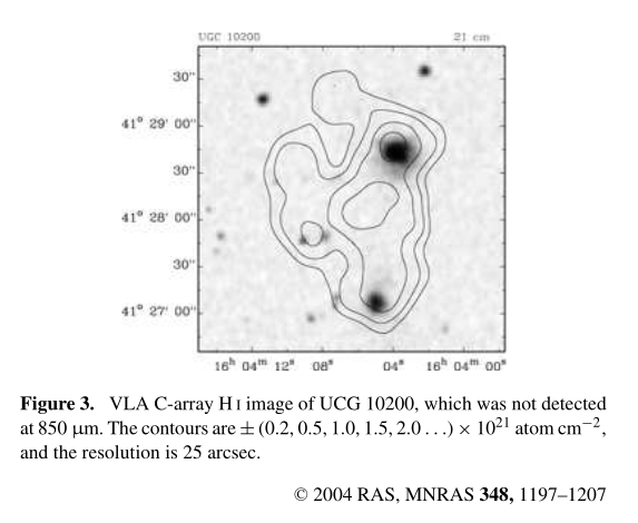
Someday I may undertake a complete census and luminosity function of the cluster system in this galaxy, and perhaps also look at the neighboring starburst galaxy UGC 10200. These systems by the way are cataloged as an interacting dwarf galaxy pair by Paudel et al. (2018) with a total stellar mass of log(M*) = 9.5 and a 3:1 mass ratio, which makes the estimated stellar mass of this galaxy just under 109 M☉. The system is very gas rich, with a neutral hydrogen mass estimated (by the same source) of 109.69 M☉. There are actually at least two published HI maps of this system. The one below, from Thomas et al. (2004) shows that atomic hydrogen extends over essentially the entire extent of the Hubble image above, including the target galaxy.
VLA map of HI gas in UGC 10200 system
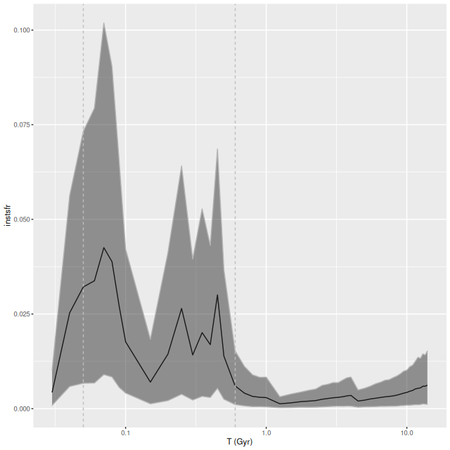
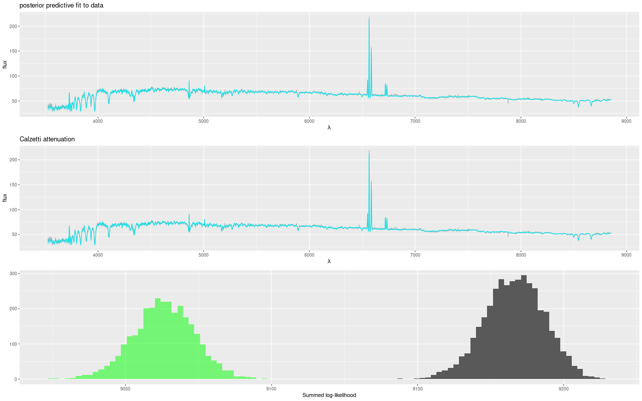
Next I turn to star formation history models for the post starburst spectrum at the top of the post. This uses the same Stan model code as my MaNGA investigations with some minor pre- and post-processing adjustments. I ran two separate models. One used a metal poor subset of the EMILES SSP libraries with Z ∈ {[-2.27], [-1.26], [-0.25]} with, as usual, Kroupa IMF and BaSTI isochrones. I did not attempt to append younger models, so the youngest age is 30Myr. For completeness I also ran a model with my usual EMILES subset + PYPOPSTAR models and Z ∈ {[-0.66], [-0.25], [+0.06], [+0.40]}. First, here is the modeled star formation history with the metal poor subset. I’ve again used a logarithmic time scale and linear star formation rate scale.
Model star formation history of central region of MCG +07-33-040 using metal poor subset of EMILES SSP library
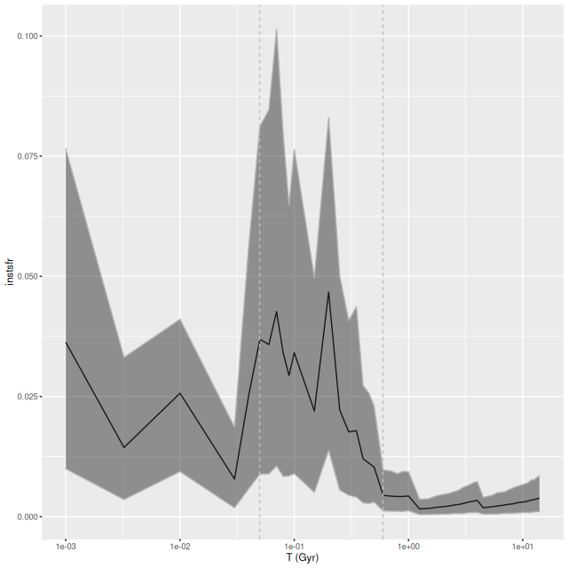
Next is the metal rich subset:
Model star formation history of central region of MCG +07-33-040 using metal rich subset of EMILES+pypopstar SSP library
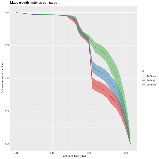
Both model runs show a fairly steep ramp up in star formation beginning at about 600Myr lookback time and a steep decline around 50Myr ago. The lingering star formation in the metal rich model might be a manifestation of the infamous “age metallicity degeneracy” since Balmer Hα emission is too low to support this level of star formation. Comparing the mass growth histories exposes a more subtle effect: the metal poor models have a consistently higher mass fraction at any given epoch. Also, the period of accelerated star formation involved a slightly smaller fraction of the present day stellar mass.
Mass growth histories of MCG +07-33-040 using metal poor and metal rich subsets of EMILES SSP library
Both models fit the data well. In terms of mean log-likelihood the metal poor model outperformed the metal rich, but only by about 0.4%. The proper Bayesian way to compare models is through the “evidence,” which is hard to estimate accurately. I suspect the metal poor model would be at least slightly flavored because it has fewer parameters than the metal rich one.
Posterior predictive fit to SDSS spectrum of MCG +07-33-040
The duration of accelerated star formation (about which both models agree) is a little surprising in light of simulations that usually show a fairly short SF burst in the first passage in mergers. But, simulations have only explored a small range of the potential parameter range. Studies of low mass galaxies with extended, massive HI haloes might be of interest.
One more sanity check. Suppose the closest approach between our target and UGC 10200 was 60Myr ago, allowing another 10Myr before (presumably) supernova feedback quenched star formation. Assuming the relative motion is transverse to our line of sight traveling 13.2 kpc in 60Myr implies an average separation speed of ≈215 km/sec. This is a perfectly reasonable value for a galaxy pair or loose group.
Finally for this spectrum, here is a quick look at emission line fluxes. Even though visually not at all obvious several lines were detected at marginal (>2σ) to high (>5σ) confidence. A couple of surprises are the [O I] 6300Å line, which is often only marginally detected even in star forming systems, is a firm (3σ) detection and stronger than the usually more prominent [O III] doublet. Also, the [S II] 6717-6730 doublet is a firm detection while the [N II] doublet is not. What this means is unclear to me. Most of the “strong emission line” metallicity indicators that I have formulae for include [N II] (or [O II] which are out of the wavelength range of these spectra), so it isn’t really possible to make a gas metallicity estimate. It’s a safe guess it’s subsolar though.
line
[Ne III] 3869
Hζ
[Ne III] 3970
Hε
Hδ
Hγ
Hβ
[O III] 4959
[O III] 5007
[O I] 6300
[O I] 6363
[N II] 6548
Hα
[N II] 6584
[S II] 6717
[SII] 6730
mean
17.1
2.3
1.5
1.6
1.9
2.1
7.9
2.4
4.9
8.2
2.8
2.9
39.1
2.5
14.4
14.2
s.d.
6.3
2.0
1.4
1.4
1.6
1.8
3.1
2.0
2.9
2.8
1.9
2.0
2.6
1.8
2.8
2.8
ratio
2.7
1.1
1.1
1.1
1.2
1.2
2.6
1.2
1.7
3.0
1.5
1.5
15.2
1.4
5.2
5.2
Flux measurements for tracked emission lines in spectrum of MCG +07-33-040. Units are 10-17 erg/sec/cm2
There are at least two questions about this galaxy that it would be nice to have answers for. First, since the SDSS fiber only includes about 7% of the luminosity and a similar fraction of the stellar mass we really don’t know if it is recently quenched globally or just where SDSS happened to target. My guess from this HST image is that it is globally quenched because its companion UGC 10200 shows clear evidence of dust lanes and extended star forming regions even in this monochromatic image, while the diffuse light in this galaxy looks relatively featureless. A definitive answer would require IFU spectroscopy though.
A second question is whether the star cluster system is truly young or primordial (or both). This would require color measurements from a return visit by HST using at least one more filter in the red. Estimating a luminosity function is feasible with the existing data, although it would have rather shallow coverage. From my casual clicking around the image it appears to be possible to reach magnitudes a little larger than +24 with reasonable precision.
When this topic first came up on the old Galaxy Zoo talk I thought these might comprise a new and overlooked category of galaxies. In fact though all of the examples I investigated belonged to cataloged galaxies and most of the spectra were of small regions in much larger nearby galaxies. A few galaxies that were in the original Virgo Cluster Catalog and excluded from the EVCC because of lack of redshift confirmation should be added back. There were probably only a few like this one with large errors in redshift estimates and high signal to noise spectra. I haven’t spent enough time with the literature to know if rapidly quenched dwarf galaxies are especially interesting. Maybe they are.
While browsing through the ADS listing of papers that cite Schawinski’s paper that I’ve been discussing for a while I came across this one by Haines et al. with the full title “Testing the modern merger hypothesis via the assembly of massive blue elliptical galaxies in the local Universe”. Besides being on the same theme of searching for post-starburst or “transitional” galaxies in the local universe that I’ve been pursuing for some time the paper was interesting because it made use of IFU based spectroscopic data that predates MaNGA. As it happens 4 of the 12 galaxies have observations in the final MaNGA release, providing an excellent opportunity to compare results from completely independent data sets.
The “modern merger hypothesis” that the authors tested relates to a topic I’ve discussed before, which is that N-body simulations show that strong, centrally concentrated starbursts are a possible outcome of major gas rich galaxy mergers around the time of coalescence. If some feedback process (an AGN or supernovae) rapidly quenches star formation there will ensue a period of time when the galaxy will be recognizable as post-starburst.
In a series of long and rather difficult (and influential judging by the number of citations) Hopkins and collaborators (2006, 2008a, 2008b) have made a case that major gas rich mergers with accompanying starbursts are in fact the major pathway to the formation of modern elliptical galaxies. They claim that their merger hypothesis accounts for a variety of phenomena, including the growth and evolution of supermassive black holes and quasars.
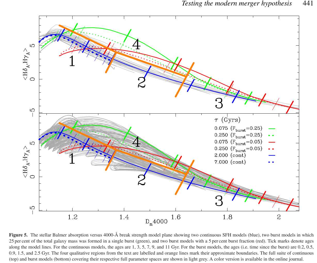
The specific aspect of the merger hypothesis this study tried to address was the prevalence of strong centrally concentrated starbursts in a sample of ellipticals in the process of forming as evidenced by visible disturbances consistent with recent mergers. The main tool they used was a suite of simple star formation history models with exponentially decaying star formation rate with single (also exponentially decaying) bursts on top of varying ages and decay time scales. They used these to predict just two quantities: Balmer absorption line strength measured by the average of the Lick HδA and HγA indexes, and the 4000Å break strength index Dn4000. For reference here is a screen grab of their model trajectories:
Predected trajectories in the Hδ – Dn4000 plane per Haines et al. (2015). Clipped from the electronic journal paper.
This is a pretty standard calculation variations of which have been performed for decades, and this graph looks much like others I have seen in the literature. A fairly basic problem with it though is that position in the Balmer – D4000 plane doesn’t uniquely constrain even the recent stellar evolution. In astronomers’ parlance there is a “degeneracy”1the term refers to a situation in which multiple combinations of some parameters of interest produce effectively equivalent values of some observable(s), or of course the converse. The best known example is the “age-metallicity degeneracy,” which refers to the fact that an old metal poor population looks like a younger metal rich one in several respects such as broad band colors. between burst strength (if any) and burst age. This is a well known problem with the Balmer line strength index that was already recognized by Worthey and Ottaviani (1997), who developed these indexes. Adding a second index in the form of the 4000Å break strength doesn’t break the degeneracy: there are regions of the plane where bursting and non-bursting populations overlap, as can be seen clearly in the graphic above. This is actually a problem for any attempt to identify post-starburst galaxies. After correcting for emission most ordinary starforming galaxies have strong Balmer absorption lines, so using that index alone will certainly produce many false positives. On the other hand selection criteria like those used by Goto and many others before and after — selecting for both strong Balmer absorption and weak emission — will capture only a small interval in post-starburst galaxies’ life cycles.
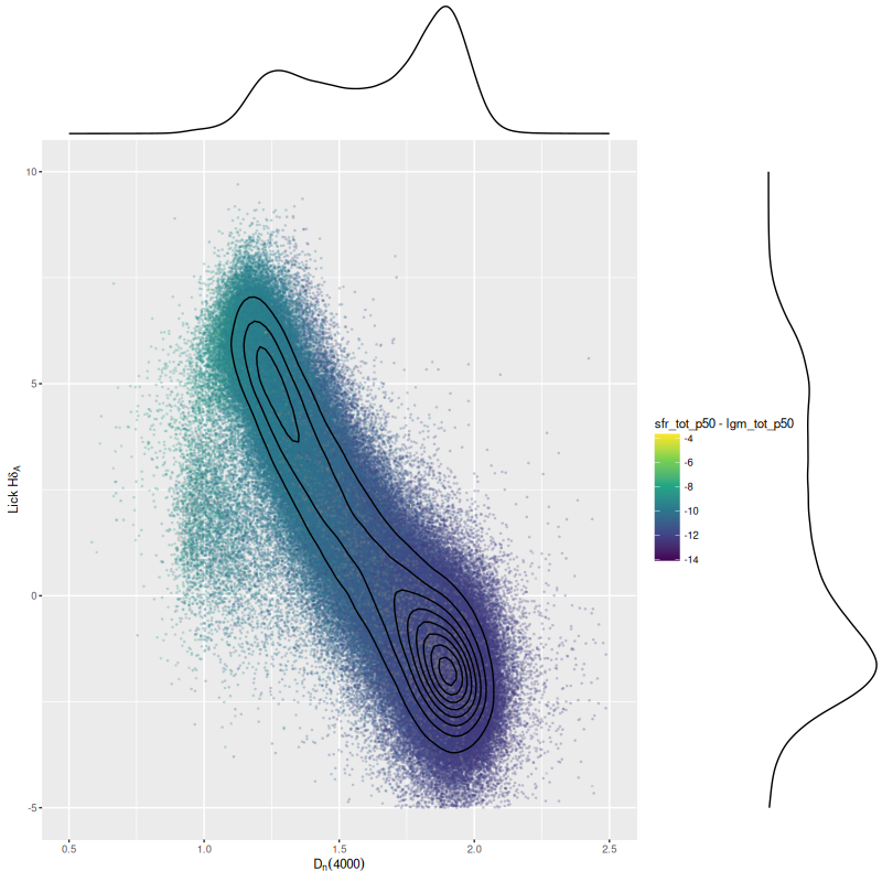
Hδ line strength vs. 4000Å break index for a large (~380K) sample of SDSS galaxy spectra. Measurements from the MPA-JHU analysis pipeline downloaded from SDSS Skyserver
Let’s get to results. Some basic details of the sample are in the table below. Morphological classifications are from McIntosh et al. (2014) as given in this paper. The abbreviations are SPM: spherical post merger; pE: peculiar Elliptical. The two marked pE/SPM didn’t have a strong consensus among several professional classifiers. I list them in order of my own visual impression of degree of disturbance. I also list redshifts taken from the MaNGA catalog and Petrosian colors.
NED name
NYU ID
mangaid
plateifu
Morph
z
u-r
g-i
NGC 3921
541044
1-617445
10510-6103
SPM
0.019
1.97
0.86
MRK 385
719486
1-604970
8940-6102
pE/SPM
0.028
1.43
0.63
MRK 366
100917
1-603309
7993-1902
pE/SPM
0.027
1.59
0.79
NGC 1149
22318
1-37155
8154-6103
pE
0.029
2.29
1.11
Columns: (1) Common catalog designation (NED name). (2) NYU VAC ID. (3) MaNGA mangaid. (4) MaNGA plateifu. (5) Morphology (see text). (6) redshift from MaNGA DRP catalog. (7-8) Petrosian u-r and g-i colors from NYU VAC via the MaNGA DRP catalog.
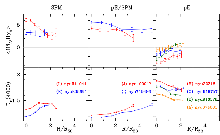
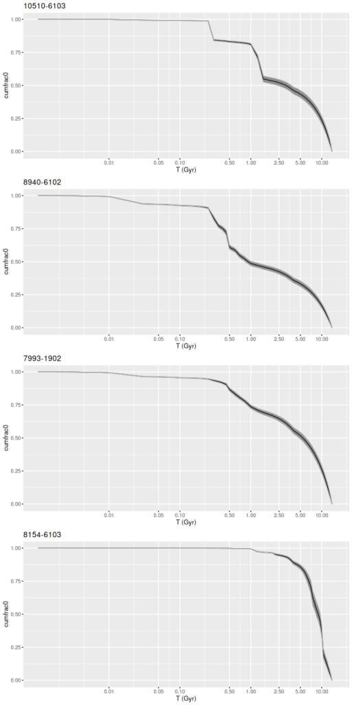
The main prediction of the merger with accompanying centrally concentrated starburst hypothesis the paper tests is that the Balmer absorption index should be large and have a negative gradient with radius while the 4000Å break strength should be low with a positive gradient. The authors concluded that only one member of their sample — nyu541044 — clearly falls in the post-starburst region (marked as region 4 in the graph above) of the <Hδ, Hγ> – Dn4000 plane. The two pE/PM galaxies, both of which are in my sample, lie in the starforming region 1. They inferred from this that these galaxies are undergoing at most a weak burst. I’m going to mildly disagree with that conclusion.
Measured values for the specified indexes from Haines et al. (2015). Clipped from the electronic journal paper.
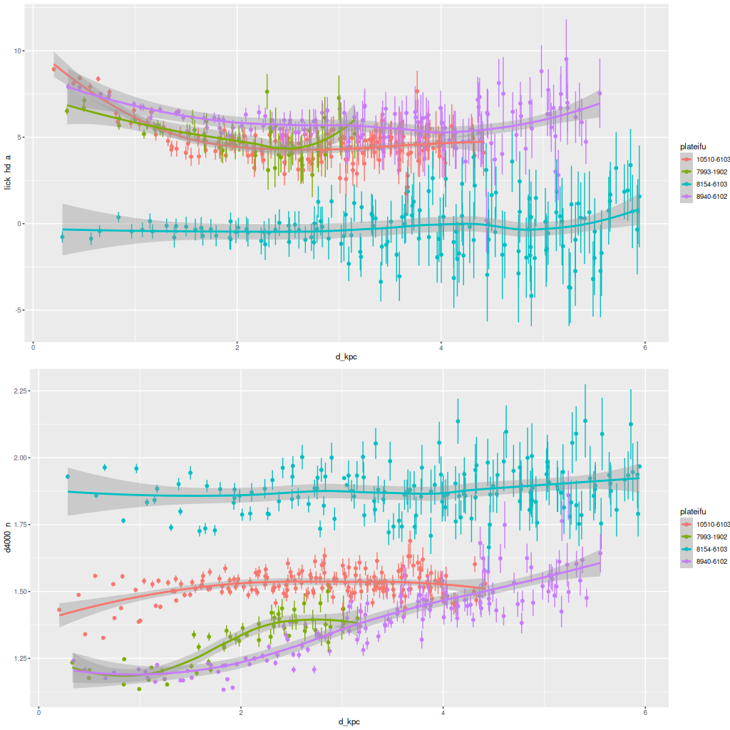
I have calculated the pseudo Lick index HδA and Dn4000 as part of my analysis “pipeline” since I started this hobby. I actually make these measurements in the initial maximum likelihood fitting step since they don’t depend on modeling except for small (usually) emission corrections. I don’t calculate an Hγ index, but its theoretical behavior is similar to Hδ. I’m trying here just to verify the approximate magnitude and radial trends of the chosen indexes. The two IFUs used in the Haines study had larger spatial coverage than these MaNGA observations (but much smaller wavelength coverage, which will become important). Instead of their strategy of binning in annuli I used my usual Voronoi binning strategy with a minimum target S/N. There were some oddities in the NYU estimates of effective radii so I chose to use distances from the IFU center in kpc for these plots. The distances assigned to the multiply binned spectra are the same as Cappelari’s published code produces; for single fiber spectra it’s just the position of the fiber center.
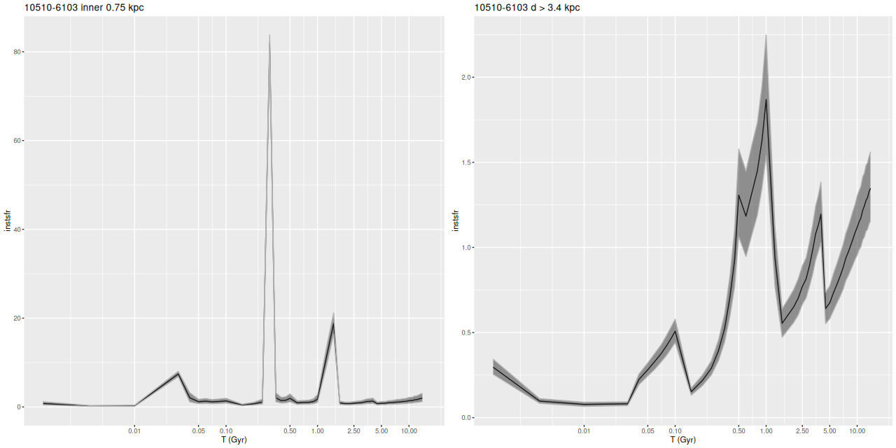
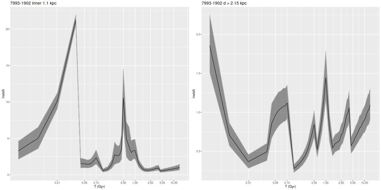
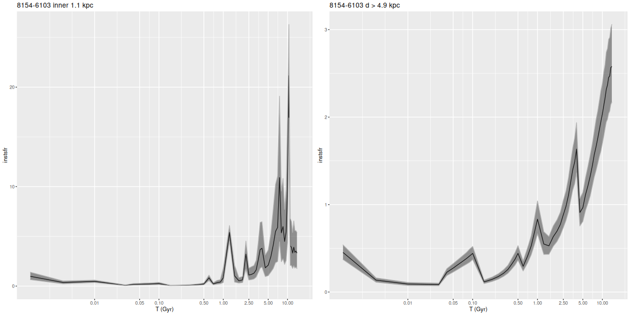
My measurements agree reasonably well with those of Haines et al. All three of the most disturbed galaxies have central Hδ indexes > 5Å with NGC 3921 (plateifu 10510-6103, nyu541044) having a larger central value and steeper gradient in the inner few kpc than the two pE/SPM galaxies. The fourth galaxy shows no obvious trend in either index with radius2The next several plots show trend lines for each galaxy computed by fitting simple loess curves to the data using the default parameters in ggplot2. These, and especially the confidence bands included in the plots, should not be taken seriously!. The central values where the S/N is highest are in good agreement.
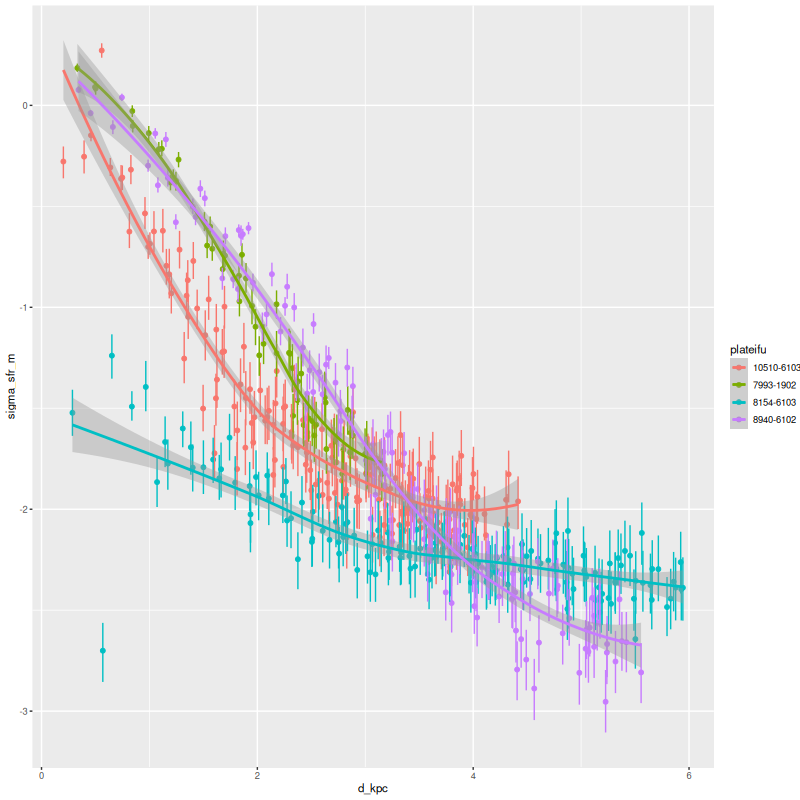
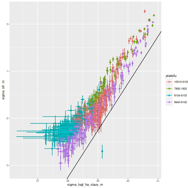
Lets turn to the results of star formation history models, which I ran on all 4 data sets. First, here are 100Myr averaged star formation rate density and specific star formation rate versus distance:
Star formation rate density vs. distance from IFU center (kpc) for 4 disturbed early type galaxies.Specific star formation rate density vs. distance from IFU center (kpc) for 4 disturbed early type galaxies.
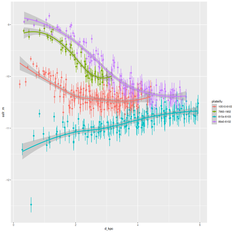
Three of these galaxies are clearly experiencing centrally concentrated episodes of star formation, and two are at or near starburst levels in specific star formation rate near their centers. As seen below two of these straddle my estimate of the “spatially resolved star forming main sequence” while the one presumed post-starburst galaxy reaches it in the central region.
Star formation rate density versus stellar mass density for 4 disturbed early type galaxies
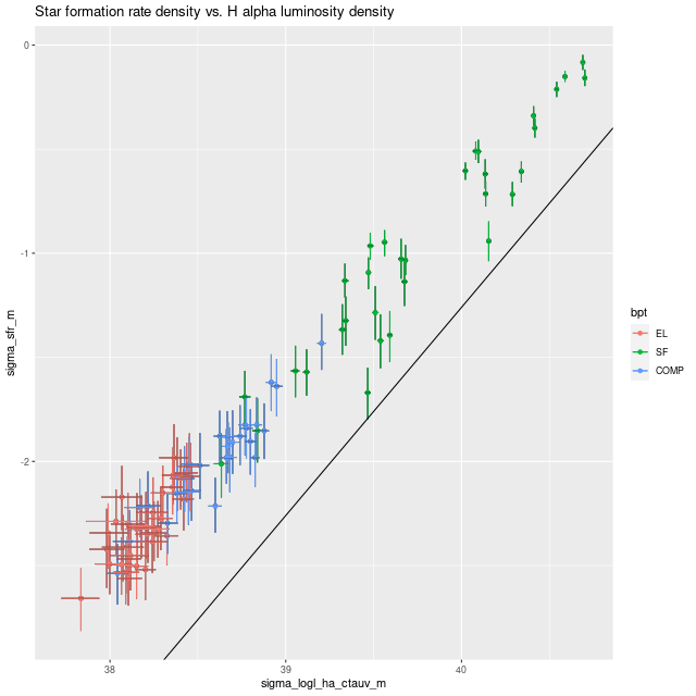
As I’ve shown several times before there’s a reasonably tight linear relationship between modeled star formation rate and Hα luminosity density. The plot shows Hα luminosity density corrected for modeled stellar redenning, which certainly underestimates attenuation in emission regions. The modeled star formation rates are consistently above the Kennicut relation shown as the straight line as I’ve seen in every sample I’ve looked at.
Star formation rate density vs. Hα luminosity density for 4 disturbed early type galaxies
Finally, lets take a look at detailed star formation histories. Instead of my usual practice of plotting them all in a grid here I just display 2 binned star formation histories. One comprises the innermost 7 bins, which since the fibers are arranged in a hexagonal grid should form a regular hexagon around the IFU center. These range in “radius” from about 0.75 to 1.1 kpc in these four galaxies. The second is for an “annulus” in approximately the outer kpc of each IFU. The extent of the IFU footprints ranges from 3.1 to 5.9 kpc. I calculate these by summing the contributions in each SFH model contributing to the bins, not by running new models for binned spectra. Since the dithered fiber positions overlaps this overestimates the total mass in each bin, but I care about the shape and timing of events rather than the absolute values of star formation rate estimates.
The next 4 plots display the results. Lookback time is logarithmically scaled with the same range and ticks for each SFH. Vertical scales are linear and differ for each graph. The graphs are in the same order as the basic information table above. As I’ve written before these models “want” to have smoothly varying mass per time bin which has the unfortunate effect of producing jumps in the apparent SFR when the bin widths change. In the BaSTI isochrone based SSP models these occur at 100 Myr, 1 Gyr, and 4 Gyr and can sometimes be quite prominent.
With caveats out of the way the one clear post-starburst in the sample had (per the model) a powerful and short starburst at ≈300 Myr lookback time, with a small amount continuing to the present (this can’t be seen at the scale of the graph, but ongoing star formation is ~1 M☉/yr). The total mass contribution from the burst and subsequent star formation is around 15%.
The two apparent ongoing starbursts have later bursts of star formation that are slightly weaker in terms of total mass contribution and peak star formation rate, but still quite significant. All three of the starburst/post-starburst galaxies appear to have had two major waves of late time (last ~2 Gyr or less) star formation. As I’ve written before in merger simulations the progenitors usually complete a few orbits before coalescence, with some enhanced star formation around each perigalactic passage. I hesitate to take these models that literally.
Turning finally to the last and least disturbed galaxy, NGC 1149, despite the bursty appearance of the SFH there’s no evidence for a major starburst in the cosmologically recent past. Whether an older starburst can be detected in this kind of modeling approach needs investigating.
One last set of graphs that may be useful. These show cumulative star formation histories — basically the cumulative sum of mass contributions starting from the oldest time bin. This is similar to a mass growth history which is a popular visualization. In my calculation of the latter the contributions are to the present day stellar mass, so an allowance for mass loss and remnant mass is made3these come from the source of the SSP models and are themselves models. Probably they are somewhat better than guesses. These things are basically black boxes to users.. The graphs are for the central regions only. Note the major virtue of these is that the contributions of major episodes of star formation can be estimated at a glance.
Cumulative star formation histories for central regions of 4 disturbed early type galaxies
To wrap up this part of the post 3 of these galaxies are compatible with the “modern merger hypothesis,” that is they have experienced centrally concentrated but spatially wide spread starbursts. The reason two of them don’t have post-starburst characteristics in the Hδ – D4000 plane is their starbursts are still underway. The current burst of star formation contributes about 5-10% of the mass in the central regions of these two. How much more is available is unknown (at least to me until I get around to finding out if there are HI mass estimates available).
Future plans: I’ve completed model runs on the 24 “post-starburst” galaxies in the MaNGA ancillary program dedicated to them. I may have something to say about them. I also may have something to say about one of the Zoogems targets that I had a small part in selecting.
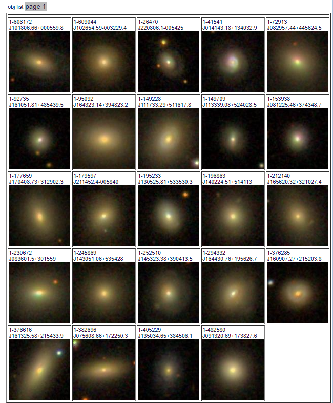
As I mentioned two posts ago there are 24 of these galaxies in the final MaNGA data release, a remarkable 11% of the full sample. I ran my SFH model code on all of these along with the prerequisite redshift offset routine1I actually completed these some time ago. I just haven’t had time to do much analysis or write about them. SDSS thumbnails of the sample are shown below. As expected none of these have significant spiral structure visible at SDSS resolution, but at least a few are noticeably disturbed.
SDSS thumbnail images of Schawinski et al.’s blue early type galaxies in MaNGA final data release (SDSS DR17)
I’m just going to discuss a few topics in this post. I’ll save a more detailed discussion for when I’ve completed analysis of the ancillary post-starburst sample, which is underway now. First, here are velocity fields calculated for the stacked RSS data, with a signal to noise cutoff of 3, the same as I used for my analysis of rotation curves of disk galaxies. Note in the graphic below the ordering is different from the image thumbnails.
Line of sight velocity fields of Schawinski et al.’s blue early type galaxies in the final MaNGA data release
By my count (based entirely on visual inspection) all but 2 of these exhibit large scale rotation, with perhaps 15 or 16 classifiable as regular rotators with the remainder containing multiple velocity components including a couple with (perhaps) kinematically distinct cores. The preponderance of rotating systems surprised me at first, but according to a review by Cappellari (2016) large scale rotation is predominant at least at lower stellar masses (Schawinski et al. characterized their sample as being “low to intermediate mass” among early type galaxies). The velocity fields indicate that many of these contain stellar disks, perhaps embedded in large bulges. That’s still consistent with classification as “early type galaxies.” Apparently the original Galaxy Zoo classification page used the term “elliptical” as the early type galaxy choice, but in the data release paper by Lintott et al. (2011) there’s a statement that the “elliptical” class should comprise ellipticals, S0’s, and perhaps Sa’s from Hubble’s classification scheme.
Depending on how my effort to do non-parametric line of sight velocity modeling goes I may return to examine the kinematics of this sample in more detail, in particular to look for evidence of gas and stellar kinematic decoupling.
Turning to the recent star formation history this sample runs the gamut from large scale starbursts to passively evolving as seen in the plot of (100 Myr averaged) star formation rate versus stellar mass density for all analyzed binned spectra (of which there were 1525 in the full sample). For reference the straight line is my estimate of the center of the local “spatially resolved star formation main sequence.” This is just a weighted least squares fit to the sample of 20 non-barred spirals with star forming BPT diagnostics that I discussed some time ago. My SFMS relation has the same slope as estimated by Bluck but is offset higher by about 0.7 dex, which probably just reflects the very different methods used to estimate star formation rates. The contour lines are the densest part of the relationship from the passively evolving Coma cluster sample that I also discussed in that post. The majority of the blue etg sample falls in the green valley, consistent with Schawinski et al.’s observation that only about 1/2 of the sample showed evidence for ongoing star formation.
“Spatially resolved” star formation rate density versus stellar mass density for 24 blue early type galaxies in final MaNGA data release. Contour lines are corresponding values for 33 passively evolving Coma cluster galaxies.
Most of the points offset the most on the high side of the SFMS come from just two galaxies: MRK 888, which I’ve discussed in the last few posts, and SDSS J014143.18+134032.8 (this is apparently not in any “classical” catalog). The legacy survey cutout below clearly shows an extended tidal tail that’s a certain sign of a relatively recent merger.
SDSS J014143.18+134032.8, a disturbed, star-bursting blue early type galaxy
I just want to take a quick look at this one: below are maps of the star formation rate density and SSFR as well as scatterplots of the same against distance from the IFU center. As with MRK 888 ongoing star formation is widespread with a peak near the center, a classic case of a merger fueled starburst. In this galaxy star formation peaks in a ring somewhat outside the nucleus. The ring can be seen clearly in the SDSS cutout and must consist of HII regions.
SDSS J014143.18+134032.8 (mangaid 1-41541; plateifu 8095-1902)
Star formation rate density and specific star formation rate – maps and scatterplots against radius in kpc.
Schawinski et al. briefly discuss the possibility that their blue ETG’s could be progenitors of E+A (aka K+A) galaxies. This galaxy and MRK 888 are plausible candidates — if star formation shut off rapidly they would certainly exhibit strong Balmer absorption for a time after emission lines disappeared since they already do. Other members of this sample are already fading towards the red sequence, and if they ever qualified as “post-starburst” it must have been in the past.
I plan to look at star formation histories in more detail after I’ve completed model runs on the MaNGA post-starburst sample.
The first iteration of Galaxy Zoo led to several collections of distinct objects, including a sample of 215 “blue early type galaxies” published in Schawinski et al. (2009)1which inexplicably and consistently says there were 204 objects while the catalog published in Vizier contains 215.I found this an interesting group of galaxies, partly because of a possible link to post-starburst (K+A) galaxies that was discussed in the original paper. The authors discuss at some length the likelihood that these are results of mergers in the cosmologically recent past, with at least one of the progenitors being gas rich. Many (at least 25% and possibly more than half) were found to be currently starforming and the rest likely to have only recently ceased forming stars as inferred from their blue colors.
The ongoing Zoogems program has 12 of Schawinski’s blue ETGs on its target list, of which 6 have been observed so far as of mid-January 2022. Somewhat surprisingly there are 24 in the final MaNGA release, over 11% of the sample!
Taking a look at the 6 with HST observations I would say none of these are typical ellipticals. Five show some degree of spiral structure although in 4 it’s embedded in a more diffuse body. One appears to me to be an S0 with both inner and outer rings — this is in agreement with the one published morphological classification I’ve found. All of the others appear more disky than ellipsoidal to me, although this is just my possibly flawed qualitative judgment. At least two are visibly disturbed. One (CGCG 315-014) is connected to a nearby galaxy with a long tidal tail as seen in the Legacy Survey thumbnail below. Markarian 888, which will be the subject of the rest of this post, has shells that extend well past the main body of the galaxy and prominent, centrally concentrated dust lanes.
CGCG 315-014 Legacy Survey Thumbnail
So far it’s the only Zoogems blue etg target with a MaNGA observation (two others on the target list are in MaNGA but of course there’s no guarantee they will ever be observed). As is often the case the IFU could have been larger — this was observed with a 37 fiber bundle giving 111 dithered spectra in the RSS file.
MRK 888 SDSS thumbnail with MaNGA IFU footprint
As always the first step in analyzing these data is to estimate redshift offsets for each spectrum, and from there we get a velocity field, which in this case shows a rapid rotator with a fairly symmetrical radial velocity pattern.
Mrk 888 (MaNGA plateifu 9894-3703) velocity field
Visual inspection suggests the line of sight velocity distribution is consistent with a rotating thin disk, so I fed the data to my Gaussian process based rotation modeling code, with results summarized below. In fact the model does an excellent job of accounting for the data, with residuals (not shown) from the model fit (top right) in a range of ±15 km/sec. One unusual feature of the velocity field is the rotation velocity turns over at somewhat less than one effective radius. Whether the rotation curve declines smoothly outside the IFU footprint or is kinematically disconnected from the outer parts of the galaxy is of course unknowable at this time.
Gaussian process rotation model results
I also ran my usual star formation history modeling code on the data binned to 97 spectra. First, here are some summary results. The stellar mass density declines roughly exponentially, which is consistent with a disky morphology:
Model estimate of stellar mass density vs. radius
Next are maps of the estimated Hα luminosity density and, on the right, the BPT classification from the [O III]/Hβ vs. [N II]/Hα diagnostic. The contours are elliptical with major axes closely aligned to the rotation axis (the posterior mean for the angle is the dashed line in the velocity field plot above). Again, the emission appears to arise in a disk.
The proper interpretation of the “composite” BPT classification is something I think I’ve written about in the past. It was originally suggested to indicate a mix of AGN and stellar ionization, but here it arises in a thin ring of weak but detectable emission just outside the star forming region. If it’s truly composite it’s likely to arise from a mix of weak star formation and ionization by hot evolved stars. In any case there’s no evidence for an AGN in the optical data.
(L) Hα luminosity density (R) BPT classification from [O III]/Hβ vs {N II]/Hα diagnostic
Next are maps of the modeled (100 Myr average) star formation rate density and specific star formation rate, and in the second row scatter plots of the same estimates against radius in kpc. The trends with radius are somewhat unusual, especially for SSFR which in a normal disk galaxy typically increases with radius even if the highest total star formation rates are centrally concentrated. Highly centrally concentrated star formation in the aftermath of mergers is predicted by some simulations.
(TL) star formation rate density; (TR) specific star formation rate; (bottom row) scatter plots vs. radius
A couple more graphs will round out my discussion of summary model estimates. As I’ve shown several times before there’s a pretty tight linear relationship between modeled SFR density and estimated Hα luminosity density. In this plot Hα is corrected for modeled stellar attenuation, which is expected always to underestimate the attenuation in emission line emitting regions. That, and the fact that Hα emission and the model star formation rate estimates probe order of magnitude different time scales probably account for the systematic offset from the standard calibration given by the straight line.
Model star formation rate density vs. Hα luminosity density corrected for stellar attenuation. Straight line is calibration from Calzetti (2012).
And, once again I show a map of the modeled optical depth of stellar attenuation. The region of highest optical depth nicely tracks the visible dust (the HST image at the top is rotated about 90º from the SDSS image). Outside the dusty region there appears to be a shallow gradient, which might indicate that the nearer side is to the northeast.
Map of modeled optical depth of stellar attenuation
Finally here are plots of the model star formation history for all spectra ordered by distance from the IFU center. In the inner 1.5 kpc or so there’s some recent burstiness with possibly a very recent acceleration of star formation. For reasons I’ve discussed recently I don’t take either the timing or magnitude of bursts of star formation too seriously, but the behavior of the models is consistent with a recent revival of star formation due presumably to a merger, for which there are multiple lines of evidence.
model star fomation histories for all spectra
With 24 of these galaxies and another 31 from the compilation of Melnick and dePropris and the post-starburst ancillary program in the final release of MaNGA these samples satisfy my criteria of being manageably sized for my computing resources while large enough to say something about the groups. So, when time permits I plan to take a look. I already have the data in hand.
I did have my old data and model runs of course, in fact they were spread over several directories on two machines. I’m going to refer to it by this catalog designation, KUG standing for the “Kiso survey of Ultraviolet-excess Galaxies.” It’s also a low power radio source with catalog entries in both FIRST and NVSS, and of course it’s in MaNGA with plateifu ID 8440-6104 (mangaid 01-216976).
In my 2018 model runs, which were interesting enough to write 3 postsabout, I found this galaxy had undergone an extraordinarily large burst of star formation that began ~1 Gyr ago with locally as much as 60% of the present day stellar mass born in the burst and something like 40% of the mass over the footprint of the IFU. In this years model runs the peak burst fraction was a considerably more modest ~25% and globally barely amounted to a slight enhancement of star formation. The starburst was also much more localized than in the earlier runs:
Fractional stellar mass in stars between 0.1 and 1.75 Gyr old in 2018 and 2021 model runs
So what happened? First, here is a comparison of modeled star formation histories for the innermost fiber, which got the largest injection of mass in the starburst.
Model star formation histories for central fiber of MaNGA plateifu 8440-6104, 2018 and 2021 model runs
The obvious remark is the double peaked starburst noted back in 2018 (and discussed at some length) has been replaced with a single narrow peak with a slow ramp up and fast decay. The peak SFR is a little larger than before but the total mass in the burst is lower.
I’ve made several changes in model formulation since 2018, of which the most important in the current context is adopting the more flexible “modified Calzetti” attenuation relation that adds an additional slope parameter to the prescription. In the current year model runs a steeper than Calzetti relation is favored throughout the IFU footprint, particularly in the central region where the starburst was strongest:
Map of modified Cal;zetti slope parameter δ — MaNGA plateifu 8440-6104
A smaller optical depth of attenuation is also favored throughout:
Modeled optical depth of attenuation – 2021 runs vs. 2018
MaNGA plateifu 8440-6104
This has a couple predictable consequences. Steeper attenuation will favor an intrinsically bluer, hence younger population while a lower optical depth requires less light, and hence mass in the stellar population. I can test this directly by returning to a model with Calzetti attenuation, and here is the result for the central fiber (this model run is labeled 2021 (c) in the legend below):
Mass growth histories –
2021 run
2021 run with Calzetti attenuation
2018 run
Central fiber of MaNGA plateifu 8440-6104
So, an eyeball analysis suggests about 3/4 of the difference between the 2018 and 2021 runs is due to the modification to the attenuation relation. The other changes I’ve made to the models are to change the stellar contribution parameters from a non-negative vector to a simplex, and at the same time changing the way I rescale the data. In early runs the SSP model fluxes were scaled to make the maximum stellar contribution ≈ 1, while the current models scale both the galaxy and SSP fluxes to ≈ 1 in the neighborhood of V, making the individual stellar contributions approximately the fraction of light contributed. An additional scale factor parameter in the model is used to adjust the overall fit. Assuming I did this right this should have no effect on a deterministic maximum likelihood solution, but with MCMC who knows?
Although the fit to the data looks about the same between the model with and without the attenuation modification the summed log-likelihood is consistently about 1% higher for the modified Calzetti model with no overlap at all in the distribution of likelihood. This suggests the case for a steeper than Calzetti attenuation is a fairly robust result.
“Posterior predictive” fits to galaxy flux data – modified Calzetti attenuation vs. Calzetti – central fiber of MaNGA plateifu 8440-6104
The galaxy flux data also changed a little bit. The early runs were on the DR14 release (version 2_1_2 of the MaNGA DRP) while the recent ones used the DR15 release (ver 2_4_3). Most of the calibration differences resemble random noise, but there is some curvature that systematically affects both the red and blue ends of the spectrum and could cause some change in the temperature distribution of the models:
Difference in measured flux from DR14 to DR15 – central fiber of MaNGA plateifu 8440-6104
While the detailed star formation histories changed, quantities that aren’t too model dependent didn’t very much. One example is shown below. Also, the kinematic maps agree with the earlier ones in detail.
Hα luminosity density – 2021 runs vs. 2018
MaNGA plateifu 8440-6104Velocity field of MaNGA plateifu 8440-6104 from 2021 model runs. Map interpolated from RSS file spectra.
One input that hasn’t changed are the emiles SSP model spectra, although there have been some procedural changes in how I handle the modeling. Early on I often used a much smaller subset of SSP models with just 27 time bins and 3 metallicities for preliminary modeling, including my first models on the same binning of these data. I also routinely ran 250 warmup iterations with just 250 more per chain. My current standard practice is always to use the largest emiles subset with 216 SSP models in 54 time bins and 4 metallicities, and I generally run 750 post-warmup iterations per chain but still with only 250 warmup iterations. This is generally enough and if adaptation fails it is usually fairly obvious. The small sample size of the earlier runs mostly effects the precision of inferences rather than means.
To conclude for now, my speculation about whether it might be possible to say something about the timing of critical events in a merger from the model star formation history was too optimistic. On a positive note though both sets of model runs retrodict that coalescence occurred at a lookback time around 500Myr ago, which is consistent with the fact that tidal tails and other merger signatures are clearly visible even in SDSS imaging. Both sets of model runs also have that odd uptick in star formation at 30Myr in the central fiber. And while the difference in burst mass contributions is a little disconcerting the current runs are more consistent with the likely gas content of ordinary spiral galaxies.
This example illustrates another well known “degeneracy” among attenuation (and adopted attenuation relation), mass, and stellar age. Whether I’ve broken the degeneracy by adopting the more flexible attenuation prescription described some time ago remains to be validated.