Category: Disk Galaxies

I haven’t had a lot of time for this hobby lately and won’t for another month or so, but I haven’t been completely inactive. When I first started modeling disk galaxy rotation curves with Gaussian processes I used a low order polynomial for the mean function. This was an admitted hack, and not a very good one at that. It’s not uncommon in the rotation curve modeling industry to adopt a functional form for the circular velocity. Sometimes it’s physically motivated (usually based on a bulge/disk/dark matter halo model), sometimes it’s purely phenomenological. With a bit of digging in the literature I found a particularly simple form in Courteau (1997):

\(v(r) = v_{0} + \frac{2}{\pi} v_{c} \arctan(r/r_{t})\)

Making this the mean function for the GP model involves just a few simple changes to the Stan code I outlined in that post. We only need two parameters for the curve, and the parameter block now looks like:

parameters {       
                
  real phi;       
                
  real<lower=0., upper=1.> cos_i;  // cosine disk inclination       
                
  real x_c;  //kinematic centers       
                
  real y_c;       
                
  real v_sys;     //system velocity offset (should be small)       
                
  real v_c;       
                
  real<lower=0> r_t;       
                
  real<lower=0.> sigma_los;       
                
  real<lower=0.> alpha;       
                
  real<lower=0.> rho;       
                
}       
                 

The key line in the model block is:

  v ~ multi_normal_cholesky(v_sys + sin_i * (2./pi() * v_c * atan(r/r_t) .* yhat ./ r), L_cov);       

And then in the generated quantities block are posterior predictions for new data at the observed points and in concentric rings:

  // model and residuals at the original points       
                
         
                
  v_rot = 2./pi() * v_c * atan(r/r_t);       
                
  vf_model = gp_pred_rng(xyhat, v-v_sys-sin_i * (v_rot .* yhat ./ r), xyhat, alpha, rho, sigma_los);       
                
  vf_model = vf_model + v_sys + sin_i * (v_rot .* yhat ./r);       
                
  vf_res = v - vf_model;       
                
         
                
  // model in rings       
                
         
                
  v_gp = gp_pred_rng(xy_pred, v-v_sys-sin_i * (v_rot .* yhat ./ r), xyhat, alpha, rho, sigma_los);       
                
  v_pred = (v_gp + sin_i * 2./pi() * v_c * atan(r_pred/r_t) .* y_pred ./ r_pred) *v_norm/sin_i;       
                
  vrot_pred[1] = 0.;       
                
  vexp_pred[1] = 0.;       
                

The full code is available in my github repository at https://github.com/mlpeck/vrot_stanmodels.

This model turned out to have very nice sampling properties using Stan’s version of NUTS, and convergence is fast enough in terms of both number of iterations and walltime to make it easily feasible to model a large sample.

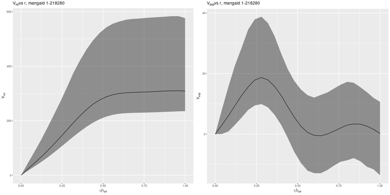
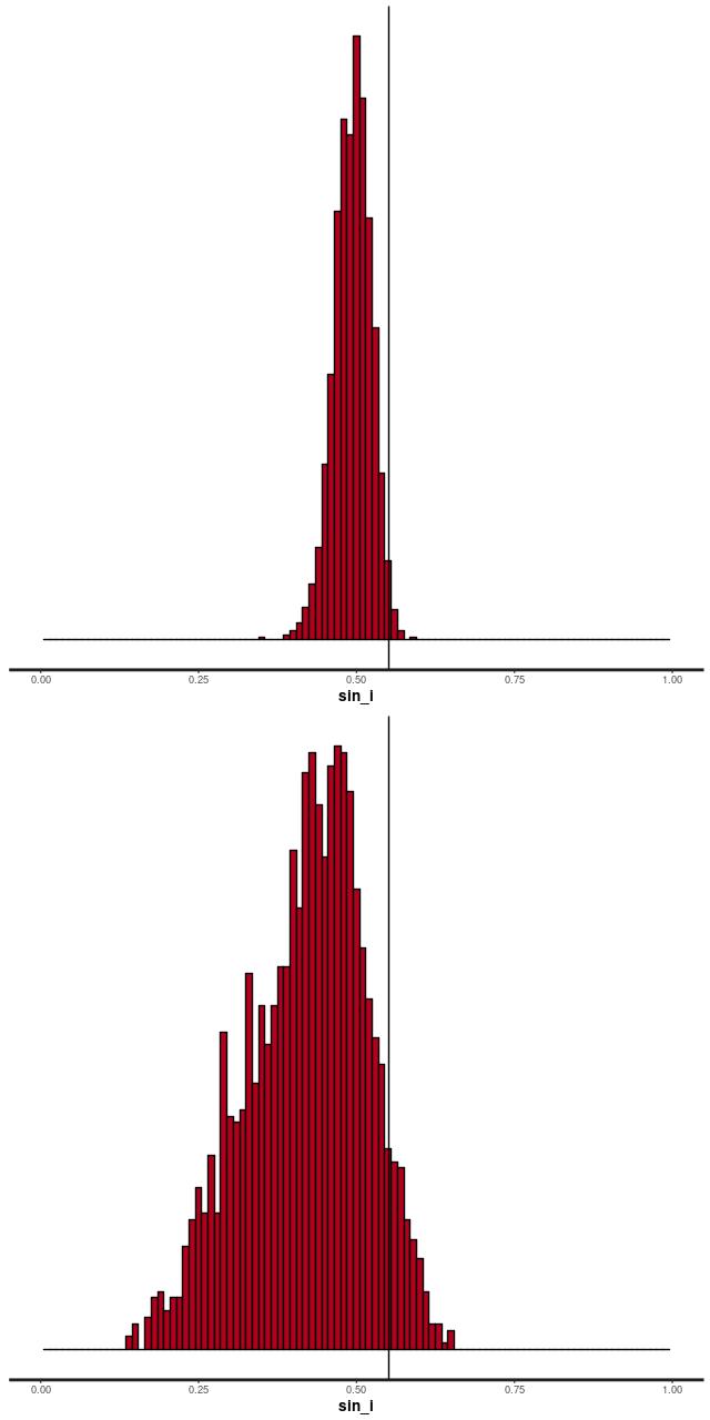
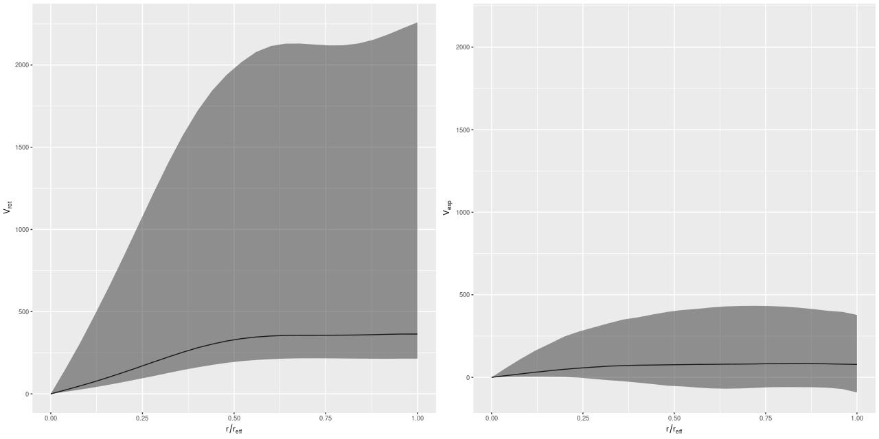
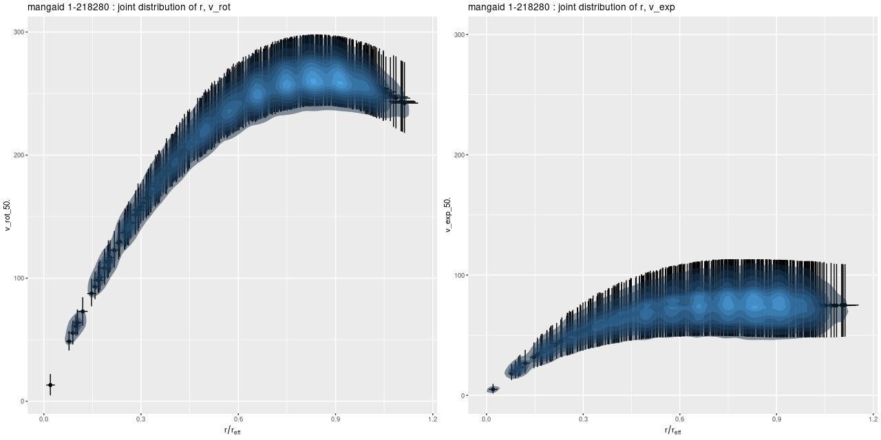
Since I’ve been using this as a running example here are posterior circular and expansion velocity estimates for plateifu 8942-12702 (mangaid 1-218280):

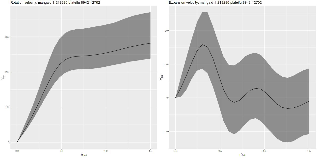
These curves are shaped just slightly differently from the ones I posted in July, but the confidence bounds are somewhat tighter. Whether this is actually due to better inference remains to be seen.

Second topic: SDSS Data release 15 went public in December as promised. I haven’t had time to dig into it much, but I did rerun the query I used to get a sample of high confidence disk galaxies based on GZ2 classifications. Run in the DR15 context that query got 588 hits, an increase of 229 from DR14 and still about 13% of the entire MaNGA galaxy sample excluding ancillary targets that aren’t also part of the main samples.

I downloaded the RSS files and have done a first pass at rotation curve modeling of the 229 new galaxies. Unfortunately I won’t have time to actually analyze what I have until, most likely, March. To conclude for now here is the kinematically most interesting example I saw from the new to DR15 sample. GZ2 classifiers called this a normal disk galaxy by a large majority

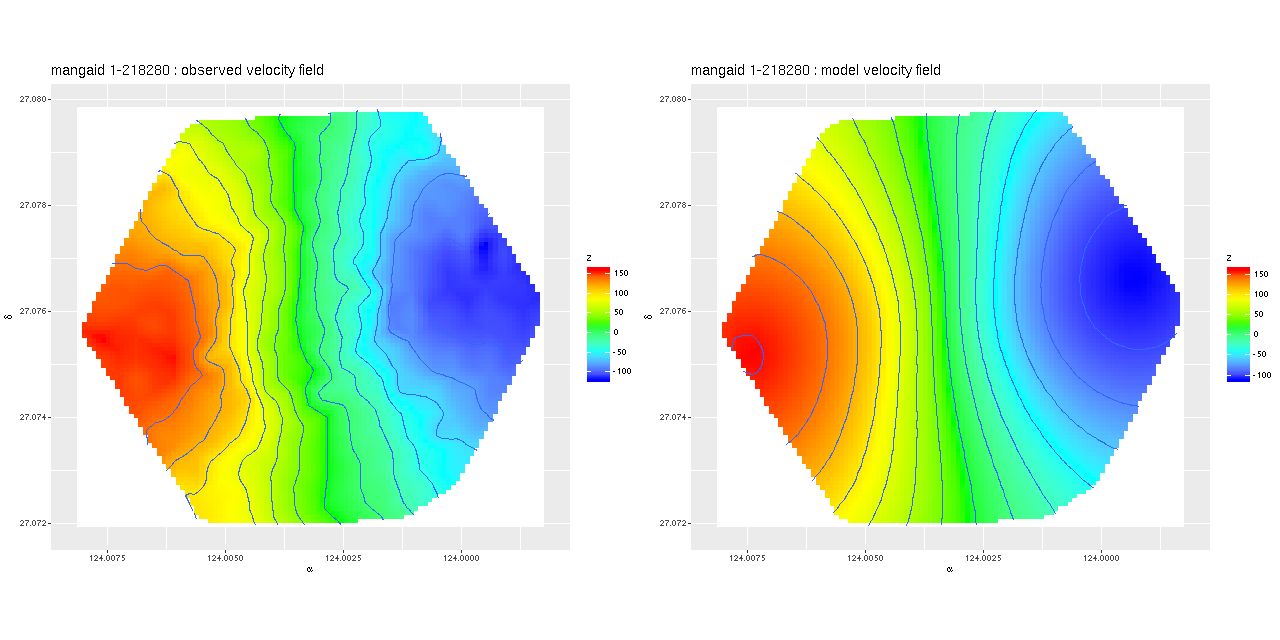
and were about evenly divided on whether it has a bar. And here is its velocity field measured from the stacked RSS file on the left, with the modeled velocity field on the right. The left graph is interpolated to the same resolution as the data cubes.

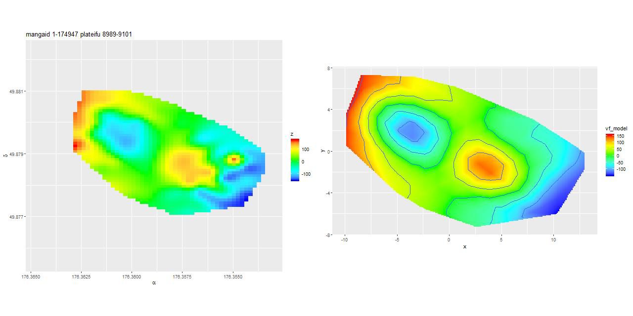
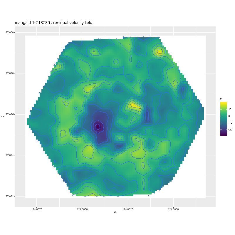
This is an incomplete map because of the signal/noise threshold I set, but it’s apparent that the outer disk is counter-rotating relative to the inner disk. This is confirmed for the stellar velocity field in the SDSS DAP, while the ionized gas rotates in the same sense as the outer disk throughout. Keep in mind that I measure blended velocities that in any given case could be dominated either by stellar light or ionized gas — in this galaxy the emission lines are very weak, so I measured the stellar velocity field. The GP based model does a good job of fitting the data, but the rotation curve isn’t exactly the standard shape:

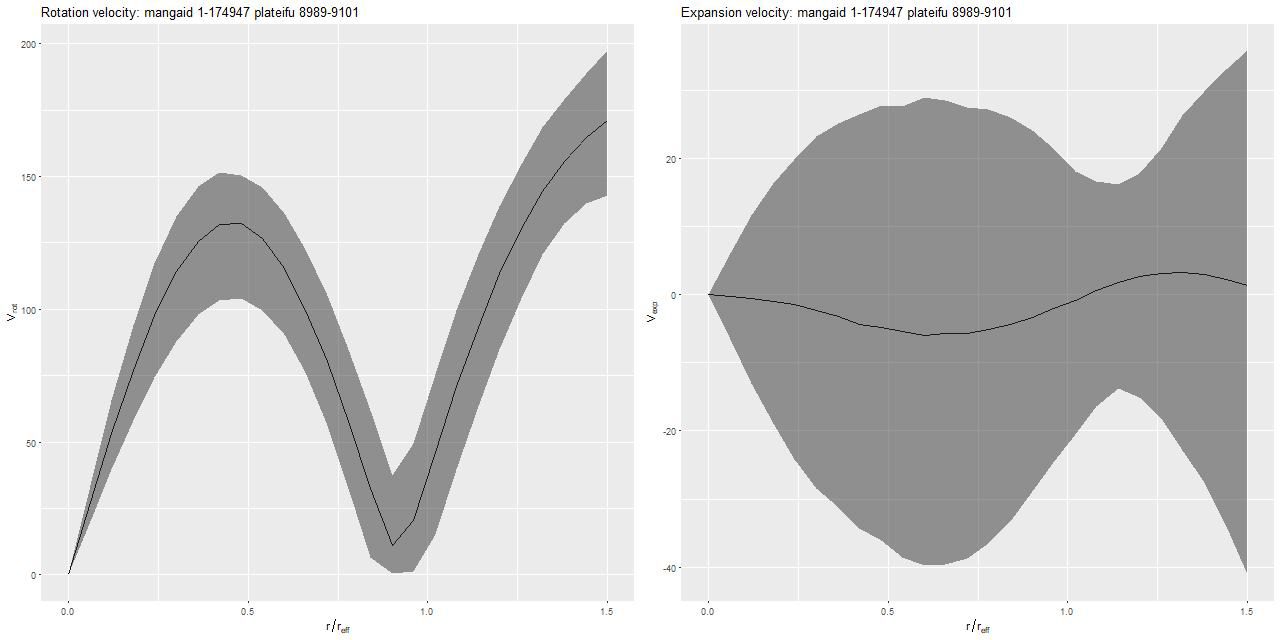
One thing this demonstrates is the versatility of the gaussian process model with a simple mean function (even if it’s wrong).

The simple polynomial model for rotation velocities that I wrote about in the last two posts seems to work well, but there are some indications of model misspecification. The relatively large expansion velocities imply large scale noncircular motions which are unexpected in an undisturbed disk galaxy (although the bar may play a role in this one), but also may indicate a problem with the model. There is also some spatial structure in the residuals, falsifying the initial assumption that residuals are iid. Since smoothing splines proved to be intractable I turned to Gaussian Process (GP) regression for a more flexible model representation. These are commonly used for interpolation and Stan offers support for them, although it’s somewhat limited in the current version (2.17.x).

I know little about the theory or practical implementation of GP’s, so I will not review the Stan code in detail. The current version of the model code is at <https://github.com/mlpeck/vrot_stanmodels/blob/master/vrot_gp.stan>. Much of the code was borrowed from tutorial introductions by Rob Trangucci and Michael Betancourt. In particular the function gp_pred_rng() was taken directly from the former with minimal modification.

There were several complications I had to deal with. First, given a vector of variates y and predictors x the gaussian process model looks something like

$$\mathbf{y} \sim \mathcal{GP}(\mathsf{m}(\mathbf{x}), \mathsf{\Sigma}(\mathbf{x}))$$

that is the GP is defined in terms of a mean function and a covariance function. Almost every pedagogical introduction to GP’s that I’ve encountered immediately sets the mean function to 0. Now, my prior for the rotation velocity definitely excludes 0 (except at r=0), so I had to retain a mean function. In order to get calculating I again just use a low order polynomial for the rotation velocity. The code for this in the model block is

  v ~ normal(v_los, dv);

  cov = cov_exp_quad(xyhat, alpha, rho);
  for (n in 1:N) {
    cov[n, n] = cov[n, n] + square(sigma_los);
  }
  L_cov = cholesky_decompose(cov);
  v_los ~ multi_normal_cholesky(v_sys + sin_i * (P * c_r) .* yhat, L_cov);

The last line looks like the previous model except that I’ve dropped the expansion velocity term because I do expect it to be small and distributed around 0. Also I replaced the calculation of the polynomial with a matrix multiplication of a basis matrix of polynomial values with the vector of coefficients. For some unknown reason this is slightly more efficient in this model but slightly less efficient in the earlier one.

A second small complication is that just about every pedagogical introduction I’ve seen presents examples in 1D, but the covariates in this problem are 2D. That turned out to be a small issue, but it did take some trial and error to find a usable data representation and there is considerable copying between data types. For example there is an N x 2 matrix Xhat which is defined as the result of a matrix multiplication. Another variable declared as row_vector[2] xyhat[N]; is required for the covariance matrix calculation and contains exactly the same values. All of this is done in the transformed parameters block.

The main objective of a gaussian process regression is to predict values of the variate at new values of the covariates. That is the purpose of the generated quantities block, with most of the work performed by the user defined function gp_pred_rng() that I borrowed. This function can be seen to implement equations 2.23-2.24 in the book “Gaussian Processes for Machine Learning” by Rasmussen and Williams 2006 (the link goes to the book website, and the electronic edition of the book is a free download). Those equations were derived for the case of a 0 mean function, but that’s not what we have here. In an attempt to fit my model into the mathematical framework outlined there I subtract the systematic part of the rotation model from the latent line of sight velocities to feed a quantity with 0 prior mean to the second argument to the posterior predictive function:

  v_gp = gp_pred_rng(xy_pred, v_los-v_sys-sin_i* (P * c_r) .* yhat, xyhat, alpha, rho, sigma_los);

then they are added back to get the predicted, deprojected, velocity field:

  v_pred = (v_gp + sin_i * (poly(r_pred, order) * c_r) .* y_pred) *v_norm/sin_i;

Yet another complication is that the positions in the plane of the disk are effectively parameters too. I don’t know if the posterior predictive part of the model is correctly specified given these complications, but I went ahead with it anyway.

The positions I want predictions for are for equally spaced angles in a set of concentric rings. The R code to set this up is (this could have been done in the transformed data block in Stan):

  n_r <- round(sqrt(N_xy))
  N_xy <- n_r^2
  rho <- seq(1/n_r, 1, length=n_r)
  theta <- seq(0, (n_r-1)*2*pi/n_r, length=n_r)
  rt <- expand.grid(theta, rho)
  x_pred <- rt[,2]*cos(rt[,1])
  y_pred <- rt[,2]*sin(rt[,1])

The reason for this is simple. If the net, deprojected velocity field is given by

$$\frac{v – v_{sys}}{\sin i} = v_{rot}(r) \cos \theta + v_{exp}(r) \sin \theta$$

then, making use of the orthogonality of trigonometric functions

$$v_{rot}(r) = \frac{1}{\pi} \int^{2\pi}_0 (v_{rot} \cos \theta + v_{exp} \sin \theta) \cos \theta \mathrm{d}\theta$$

and

$$v_{exp}(r) = \frac{1}{\pi} \int^{2\pi}_0 (v_{rot} \cos \theta + v_{exp} \sin \theta) \sin \theta \mathrm{d}\theta$$

The next few lines of code just perform a trapezoidal rule approximation to these integrals:

  vrot_pred[1] = 0.;
  vexp_pred[1] = 0.;
  for (n in 1:N_r) {
    vrot_pred[n+1] = dot_product(v_pred[((n-1)*N_r+1):(n*N_r)], cos(theta_pred[((n-1)*N_r+1):(n*N_r)]));
    vexp_pred[n+1] = dot_product(v_pred[((n-1)*N_r+1):(n*N_r)], sin(theta_pred[((n-1)*N_r+1):(n*N_r)]));
  }
  vrot_pred = vrot_pred * 2./N_r;
  vexp_pred = vexp_pred * 2./N_r;

These are then used to reconstruct the model velocity field and the difference between the posterior predictive field and the systematic portion of the model:

  for (n in 1:N_r) {
    v_model[((n-1)*N_r+1):(n*N_r)] = vrot_pred[n+1] * cos(theta_pred[((n-1)*N_r+1):(n*N_r)]) +
                                     vexp_pred[n+1] * sin(theta_pred[((n-1)*N_r+1):(n*N_r)]);
  }
  v_res = v_pred - v_model;

Besides some uncertainty about whether the posterior predictive inference is specified properly there is one very important problem with this model: the gradient computation, which tends to be the most computationally intensive part of HMC, is about 2 orders of magnitude slower than for the simple polynomial model discussed in the previous posts. The wall time isn’t proportionately this much larger because fewer “leapfrog” steps are typically needed per iteration and the target acceptance rate can be set to a lower value. This still makes analysis of data cubes quite out of reach, and as yet I have only analyzed a small number of galaxies’ RSS based data sets.

Here are some results for the sample data set from plateifu 8942-12702. This galaxy is too big for its IFU — the cataloged effective radius is 16.2″, which is about the radius of the IFU footprint. Therefore I set the maximum radius for predicted values to 1r_eff.

The most important model outputs are the posterior predictive distributions for the rotational and expansion velocities:

The rotational velocity is broadly similar to the polynomial model, but it has a very long plateau (the earlier model was beginning to turn over by 1 r_eff) and much larger uncertainty intervals. The expansion velocity curve displays completely different behavior from the polynomial model (note that the vertical scales of these two graphs are different). The mean predicted value is under 20 km/sec everywhere, and 0 is excluded only out to a radius around 6.5″, which is roughly the half length of the bar.

The reason for the broad credible intervals for the rotation velocity in the GP model compared to the polynomial model can be seen by comparing the posteriors of the sine of the inclination angle. The GP model’s is much broader and has a long tail towards very low inclinations. This results in a long tail of very high deprojected rotational velocities. Both models favor lower inclinations than the photometric estimate shown as a vertical line.

I’m going to leave off with one more graph. I was curious if it was really necessary to have a model for the rotation velocity, so I implemented the common pedagogical case of assuming the prior mean function is 0 (actually a constant to allow for an overall system velocity). Here are the resulting posterior predictive estimates of the rotation and expansion velocities:

Conclusion: it is. There are several other indications of massive model failure, but these are sufficient I think.

In a future post (maybe not the next one) I’ll discuss an application that could actually produce publishable research.

I’m going to take a selective look at some of the Stan code for this model, then show some results for the RSS derived data set. The complete stan file is at <https://github.com/mlpeck/vrot_stanmodels/blob/master/vrot.stan>. By the way development is far from frozen on this little side project, so this code may change in the future or I may add new models. I’ll try to keep things properly version controlled and my github repository in sync with my local copy.

Stan programs are organized into named blocks that declare and sometimes operate on different types of variables. There are seven distinct blocks that may be present — I use 6 of them in this program. The functions block in this program just defines a function that returns the values of the polynomial representing the rotational and expansion velocities. The data block is also straightforward:

data {
int<lower=1> order; //order for polynomial representation of velocities
int<lower=1> N;
vector[N] x;
vector[N] y;
vector[N] v; //measured los velocity
vector[N] dv; //error estimate on v
real phi0;
real<lower=0.> sd_phi0;
real si0;
real<lower=0.> sd_si0;
real<lower=0.> sd_kc0;
real<lower=0.> r_norm;
real<lower=0.> v_norm;
int<lower=1> N_r; //number of points to fill in
vector[N_r] r_post;
}

The basic data inputs are the cartesian coordinates of the fiber positions as offsets from the IFU center, the measured radial velocities, and the estimated uncertainties of the velocities. I also pass the polynomial order for the velocity representations and sample size as data, along with several quantities that are used for setting priors.

The parameters block is where the model parameters are declared, that is the variables we want to make probabilistic statements about. This should be mostly self documenting given the discussion in the previous post, but I sprinkle in some C++ style comments. I will get to the length N vector parameter v_los shortly.

parameters {
  real phi;
  real<lower=0., upper=1.> sin_i;  // sine disk inclination
  real x_c;  //kinematic centers
  real y_c;
  real v_sys;     //system velocity offset (should be small)
  vector[N] v_los;  //latent "real" los velocity
  vector[order] c_rot;
  vector[order] c_exp;
  real<lower=0.> sigma_los;
}

In this program the transformed parameters block mostly performs the matrix manipulations I wrote about in the last post. These can involve both parameters and data. A few of the declarations here improve efficiency in minor but useful ways recommended in the Stan help forums by members of the development team. For example the statement real sin_phi = sin(phi); saves recalculating the sine further down.

transformed parameters {
  vector[N] xc = x - x_c;
  vector[N] yc = y - y_c;
  real sin_phi = sin(phi);
  real cos_phi = cos(phi);
  matrix[N, 2] X;
  matrix[N, 2] Xhat;
  matrix[2, 2] Rot;
  matrix[2, 2] Stretch;
  vector[N] r;
  vector[N] xhat;
  vector[N] yhat;

  X = append_col(xc, yc);
  Rot = [ [-cos_phi, -sin_phi],
          [-sin_phi, cos_phi]];
  Stretch = diag_matrix([1./sqrt(1.-sin_i^2), 1.]');
  Xhat = X * Rot * Stretch;
  xhat = Xhat[ : , 1];
  yhat = Xhat[ : , 2];
  r = sqrt(yhat .* yhat + xhat .* xhat);
}

The model block is where the log probability is defined, which is what the sampler is sampling from:

model {
  phi ~ normal(phi0, sd_phi0);
  sin_i ~ normal(si0, sd_si0);
  x_c ~ normal(0, sd_kc0/r_norm);
  y_c ~ normal(0, sd_kc0/r_norm);
  v_sys ~ normal(0, 150./v_norm);
  sigma_los ~ normal(0, 50./v_norm);
  c_rot ~ normal(0, 1000./v_norm);                                                                        
  c_exp ~ normal(0, 1000./v_norm);

  v ~ normal(v_los, dv);
  v_los ~ normal(v_sys + sin_i * (
                  sump(c_rot, r, order) .* yhat + sump(c_exp, r, order) .* xhat),
                  sigma_los);
}

I try to be consistent about setting priors first in the model block and using proper priors that are more or less informative depending on what I actually know. In this case some of these are hard coded and some are passed to Stan as data and can be set by the user. I find it necessary to supply fairly informative priors for the orientation and inclination angles. For the latter it’s because of the weak identifiability of the inclination. For the former it’s to prevent mode hopping.

Stan’s developers recommend that parameters should be approximately unit scaled, and this usually entails rescaling the data. In this case we have both natural velocity and length scales. Typical peculiar velocities are on the order of no more than a few hundreds of km/sec., so I scale them to units of 100 km/sec. The MaNGA primary sample is intended to have each galaxy observed out to 1.5R_eff, where R_eff is the (r band) half light radius, so the maximum observed radius should typically be ∼1.5R_eff. Therefore I typically divide all position measurements by that amount with the effective radius taken from nsa_elpetro_th50_r in drpcat. Other catalog values that I use as inputs to the model are nsa_elpetro_phi for the orientation angle and nsa_elpetro_ba for the cosine of the inclination. These are used as the central values of the priors and also to initialize the sampler.

Once I solved the problem of parametrizing angles the next source of pathologies I encountered was a tendency towards multimodal kinematic centers. This usually manifests as one or more chains being displaced from the others rather than mode hopping within a chain, although that can happen too. In the typical case the extra modes would place the center in an adjacent fiber to the one closest to the IFU center, but sometimes much larger jumps happen. Although I wouldn’t necessarily rule out the possibility of actual multimodality when it happens it has a severe effect on convergence diagnostics and on most other model parameters. I therefore found it necessary to place a tighter prior on the kinematic centers than I would have liked based solely on prior knowledge: the default prior puts about 95% of the prior mass within the radius of the central fiber. This could overconstrain the kinematic center in some cases, particularly low mass galaxies with weak central concentration.

A very common situation with astronomical data is to have quantities measured with error with an accompaying uncertainty estimate for each measurement. My code for estimating redshift offsets kicks out an uncertainty estimate, so this is no exception. I take a standard approach to modeling this: the unknown “true” line of sight velocity is treated as a latent variable, with the measured velocity generated from a distribution having mean equal to the latent variable and standard deviation the estimated uncertainty. In this case the distribution is assumed to be Gaussian. The latent variable is then treated as the response variable in the model. Since I had no particular expectations about what the residuals from the model should look like I fell back on the statistician’s standard assumption that they are independent and identically distributed gaussians with standard deviation to be estimated as part of the model.

Having a latent parameter for every measurement seems extravagant, but in fact it causes no issues at all except for a slight performance penalty. With the distributional assumptions I made the latent variables can be marginalized out and posteriors for the remaining parameters will be the same within typical Monte Carlo variability. The main performance difference seems to arise from slower adaptation in the latent variables version.

Finally, some results from the observation with plateifu 8942-12702 (mangaid 1-218280). First, the measured velocity field and the posterior mean model. The observations came from the same data shown in the previous post interpolated onto a finer grid.

The model seems not too bad except for missing some high spatial frequency details. The residuals may be revealing (again this is the posterior mean difference between observations and model):

There is a strong hint of structure here, with a ridge of positive residuals that appears to follow the inner spiral arms at least part of the way around. There are also two regions of larger than normal residuals on opposite sides of the nucleus and with opposite signs. In this case they appear to be at or near the ends of the bar. This is a common feature of these maps — I will show another example or two later.

Next are the joint posterior distributions of \(v_{rot}\) with radius r and \(v_{exp}\) with r. Error bars are 95% credible intervals.

The rotation curve seems not unrealistic given the limited expressiveness of the polynomial model. The initial rise is slow compared to typical examples in the literature, but this is probably attributable to the limited spatial resolution of the data. The peak value is completely reasonable for a fairly massive spiral. The expansion velocity on the other hand is surprising. It should be small, but it’s not especially so. Nowhere do the error bars include 0.

There are a number of graphical tools that are useful for assessing MCMC model performance. Here are some pairs plots of the main model parameters:

There are several significant correlations here, none of which are really surprising. The polynomial coefficients are strongly correlated. The inclination angle is strongly correlated with rotation velocity and slightly less, but still significantly correlated with expansion velocity. The orientation angle is slightly correlated with rotation velocity but strongly correlated with expansion. The estimated system velocity is strongly correlated with the x position of the kinematic center but not y — this is because the rotation axis is nearly vertical in this case. The relatively high value of v_sys (posterior mean of 25 km/sec) is a bit of a surprise since the SDSS spectrum appeared to be well centered on the nucleus and with an accurate redshift measurement. Nevertheless the value appears to be robust.

Stan is quite aggressive with warnings about convergence issues, and it reported none for this model run. No graphical or quantitative diagnostics indicated any problems. Nevertheless there are several indicators of possible model misspecification.

1. Signs of structure in residual maps are interesting because they indicate perturbations of the velocity field as small as ∼10 km/sec by spiral structure or bars may be detectable. But it also indicates the assumption of iid residuals is false.
2. It’s hard to tell from visual inspection if the symmetrically disposed velocity residuals near the nucleus are due to rotating rings of material or streaming motions, but in any case a low order polynomial can’t be fit to them. I will show more dramatic examples of this in a future post.
3. Large scale expansion (or contraction) shouldn’t be seen in a disk galaxy, but the estimated expansion velocity is rather high in this case. Perturbations by the rather prominent bar would indicate that a model with a \(2 \theta\) angular dependence should be explored.

Next up, a possible partial solution.

 

In the course of studying star formation histories I’ve accumulated lots of velocity fields similar to the ones I just posted about. For purposes of SFH modeling their only use is to reduce wavelengths to the galaxy rest frame. It’s not sufficient just to use the system redshift because peculiar velocities of a few hundred km/sec (typical for disk galaxies) translate into spectral shifts of 2-3 pixels, enough to seriously impair spectral fits. Naturally however I wanted to do something else with these data, so I decided to see if I could model rotation curves. And, since I’m interested in Bayesian statistics and was using it anyway, I decided to try Stan as a modeling tool. This is hardly a new idea; in fact I was motivated in part by a paper I encountered on arxiv by Oh et al. (2018), who attempt a more general version of essentially the same model.

The basic idea behind these models is that if the stars and/or gas are confined to a thin disk and moving in its plane we can recover their full velocities from the measured radial velocities when the plane of the galaxy is tilted by a moderate amount to our line of sight (inclination angles between about 20^o and 70^o are generally considered suitable). The equations describing the tilted disk model are given in, among many other places,  Teuben (2002). I reproduce them here with some minor notational changes. The crude sketch below might or might not make the geometry of this a little clearer. The galaxy is inclined to our line of sight by some angle \(i\)  (where 0 is face-on), with the position angle of the receding side \(\phi\), by convention measured counterclockwise from north. The observed radial velocity \(v(x,y)\) at cartesian coordinates \((x,y)\) in the plane of the sky can be written in terms of polar coordinates \((r, \theta)\) in the plane of the galaxy as

$$v(x,y) = v_{sys} +  \sin i  (v_{rot} \cos \theta + v_{exp} \sin \theta) $$

where

$$\sin \theta = \frac{- (x-x_c)  \cos \phi – (y-y_c) \sin \phi}{r \cos i}$$

$$\cos \theta = \frac{ – (x-x_c) \sin \phi + (y-y_c) \cos \phi}{r}$$

and \(v_{sys}, v_{rot}, v_{exp}\) the overall system velocity at the kinematic center \((x_c, y_c)\), rotational (or transverse), and expansion (or radial) components of the measured line of sight velocity.

 

The transformation between coordinates on the sky and coordinates in the plane of the galaxy can be written as a sequence of vector and matrix operations consisting of a translation, rotation, and a stretch:

$$[\hat x, \hat y] = [(x – x_c), (y-y_c)] \mathbf{R S}$$

$$ \mathbf{R} = \left( \begin{array}{c} -\cos \phi & -\sin \phi \\ -\sin \phi & \cos \phi \end{array} \right)$$

$$ \mathbf{S} = \left( \begin{array}{c} 1/\cos i & 0\\ 0 & 1 \end{array} \right)$$

and now the first equation above relating the measured line of sight velocity to velocity components in the disk can be rewritten as

$$v(x, y) = v_{sys} + \sin i [v_{rot}(\hat x, \hat y) \hat y/r + v_{exp}(\hat x, \hat y) \hat x/r]$$

Note that I am defining, somewhat confusingly,

$$\cos \theta = \hat y/r \\ \sin \theta = \hat x/r$$

with

$$r = \sqrt{\hat x^2 + \hat y^2}$$

This is just to preserve the usual convention that the Y axis points up, while also preserving the astronomer’s convention that angles are measured counterclockwise from north.

Stan supports a full complement of matrix operations and it turns out to be slightly more efficient to code these coordinate transformations as matrix multiplications, even though it involves some copying between different data types.

So far this is just geometry. What gives the model physical content is that both \(v_{rot}\) and \(v_{exp}\) are assumed to be strictly axisymmetric. This seems like a very strong assumption, but these can be seen as just the lowest order modes of a Fourier expansion of the velocity field. There’s no reason in principle why higher order Fourier terms can’t be incorporated into the model. The appropriateness of this first order model rests on whether it fits the data and its physical interpretability.

How to represent the velocities posed, and continues to pose, a challenge. Smoothing splines have desirable flexibility and there’s even a lengthy case study showing how to implement them in Stan. I tried to adapt that code and found it to be quite intractable, the problem being that coordinates in the disk frame are parameters, not data, so the spline basis has to be rebuilt at each iteration of the sampler.

In order to get started then I just chose a polynomial representation. This isn’t a great choice in general because different orders of the polynomial will be correlated which leads to correlated coefficient estimates. If the polynomial order chosen is too high the matrix of predictors becomes ill conditioned and data can be overfit. This is true for both traditional least squares and Bayesian methods. The minimum order to be included is linear, because both \(v_{rot}\) and \(v_{exp}\) have limiting values of 0 at radius 0. This is both because of continuity and identifiability: a non-zero velocity at 0 is captured in the scalar parameter \(v_{sys}\). It takes at least a 3rd order polynomial to represent the typical shape of a rotation curve; I found that convergence issues started to become a problem at as low as 4th order, so I just picked 3rd order for the models reported here. In the next or a later post I will show a partial solution to a more flexible representation, and I may revisit this topic in the future.

There are two angles in the model, and this presents lots of interesting complications. First, it’s reasonable to ask if these should be treated as data or parameters of the model. There are useful proxies for both in the photometric data provided in the MaNGA catalog, in fact there are several. Some studies do in fact fix their values. I think this is both a conceptual and practical error. First, these are photometric measurements not kinematic ones. They aren’t the same thing. Second, they are subject to uncertainty, possibly a considerable amount. Failing to account for that could lead to seriously underestimated uncertainties in the velocities. In fact I think much of the literature is significantly overoptimistic about how well constrained are rotation velocities.

So, both the inclination and major axis orientation are parameters. And this immediately creates other issues. Hamiltonian Monte Carlo requires gradient evaluation, and the version implemented in Stan requires the gradient to exist everywhere in \(\mathbb{R}^N\). Bounded parameters are automatically transformed to create new, unbounded ones. But this creates an acknowledged problem that circles can’t be mapped to the real line, at least in a way that preserves probability measure everywhere. There are a couple potential ways to avoid this problem, and I chose different ones for the inclination and orientation angles.

The inclination turned out to be the easier to deal with, at least in terms of model specification. First, the inclination angle is constrained to be between 0 and 90^o. Instead of the angle itself I make the parameter \(\sin i\) (or \(\cos i\); it turns out to make no difference at all which is used). This is constrained to be between 0 and 1 in its declaration. Stan maps this to the real line with a logistic transform, so the endpoints map to \(\mp \infty\). But that creates no issue in practice because recall this model is only applicable to disk galaxies with moderate inclination. Rotation can’t be measured at all in an exactly face on galaxy. Rotation is all that can be measured in an exactly edge on one, but this model is misspecified for that case. If contrary to expectations the posterior wants to pile up near 0 or 1 it tells us either that something is wrong with the model or data or that the actual inclination is outside the usable range.

Even though the parametrization is straightforward inference about the inclination can be problematic because it is only weakly identified: notice it enters the velocity equation multiplicatively so, for example, halving it’s value and simultaneously doubling both velocity components produces exactly the same likelihood value. Identifiability therefore is only achieved through the stretch operation and through the prior.

There are two possible ways to parametrize the orientation angle, which is determined modulo \(2 \pi\). I chose to make the angle the parameter and to leave it unbounded. This creates a form of what statisticians call a label switching problem: suppose we try an improper uniform prior for this parameter (generally not a good idea), and suppose there’s a mode in the posterior at some angle \(\hat \phi\). Then there will be other modes at \(\hat \phi \pm \pi\) with the signs of the velocities flipped, and at \(\hat \phi \pm \pi/2\) with \(v_{rot}\) taking the role of \(v_{exp}\) and vice versa. Therefore even if there’s a well behaved distribution around \(\hat \phi\) it will be replicated infinitely many times, making the posterior improper. The solution to this is to introduce a proper prior and in practice it has to be informative enough to keep the sampler from hopping between modes.

Since the orientation angle enters the model only through its cosine and sine the other solution available in Stan is to declare the cosine/sine pair as a 2 dimensional unit vector. This solves the potential improper posterior problem, but it doesn’t solve the mode hopping problem; a moderately informative prior is still needed to keep the elements of the vector from flipping signs.

I’ve tried both the direct parameterization and the unit vector version, and both work with appropriate priors. I chose the former mostly because I expect the angle to have a fairly symmetrical posterior, which makes a gaussian prior a reasonable choice.  Choosing a prior for the unit vector that makes the posterior of the angle symmetrical seems a trickier task. It turns out that the data usually has a lot to say about the orientation angle, so as long as mode hopping is avoided its effect on inferences is much less problematic than the inclination.

Well, I’ve been more verbose than expected, so again I’ll stop the post halfway through. Next time I’ll take a selective look at the code and some results from the data set introduced last time.