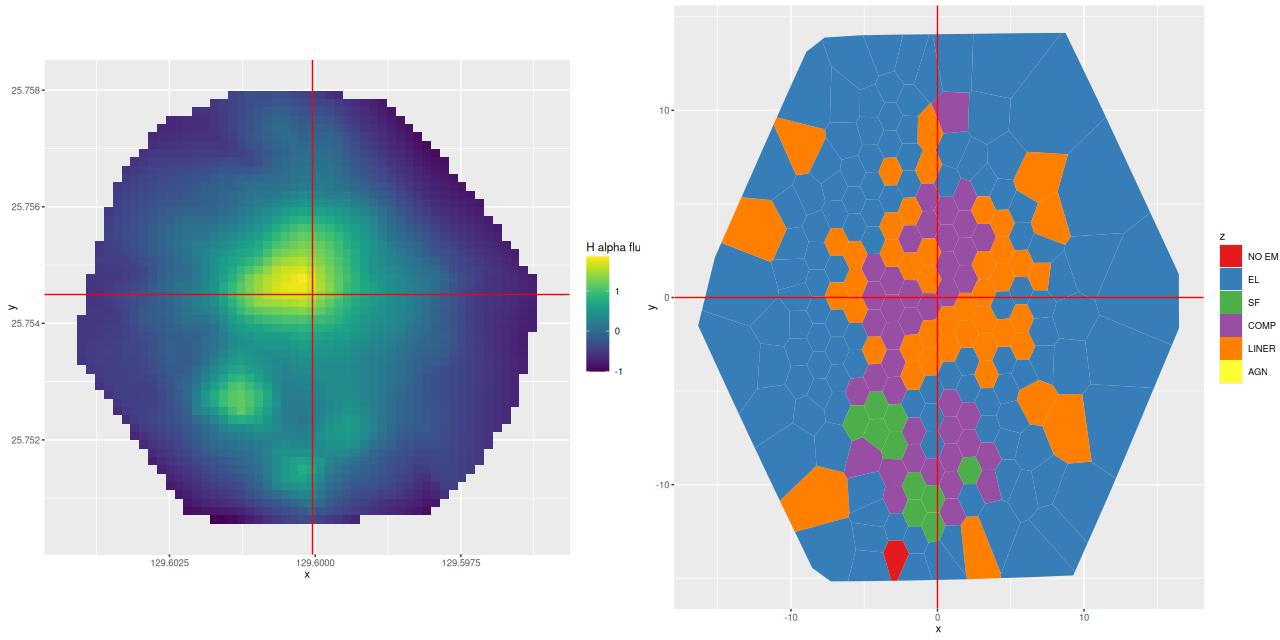
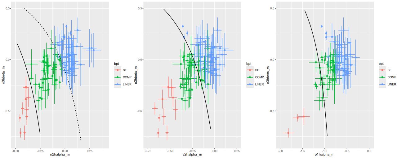
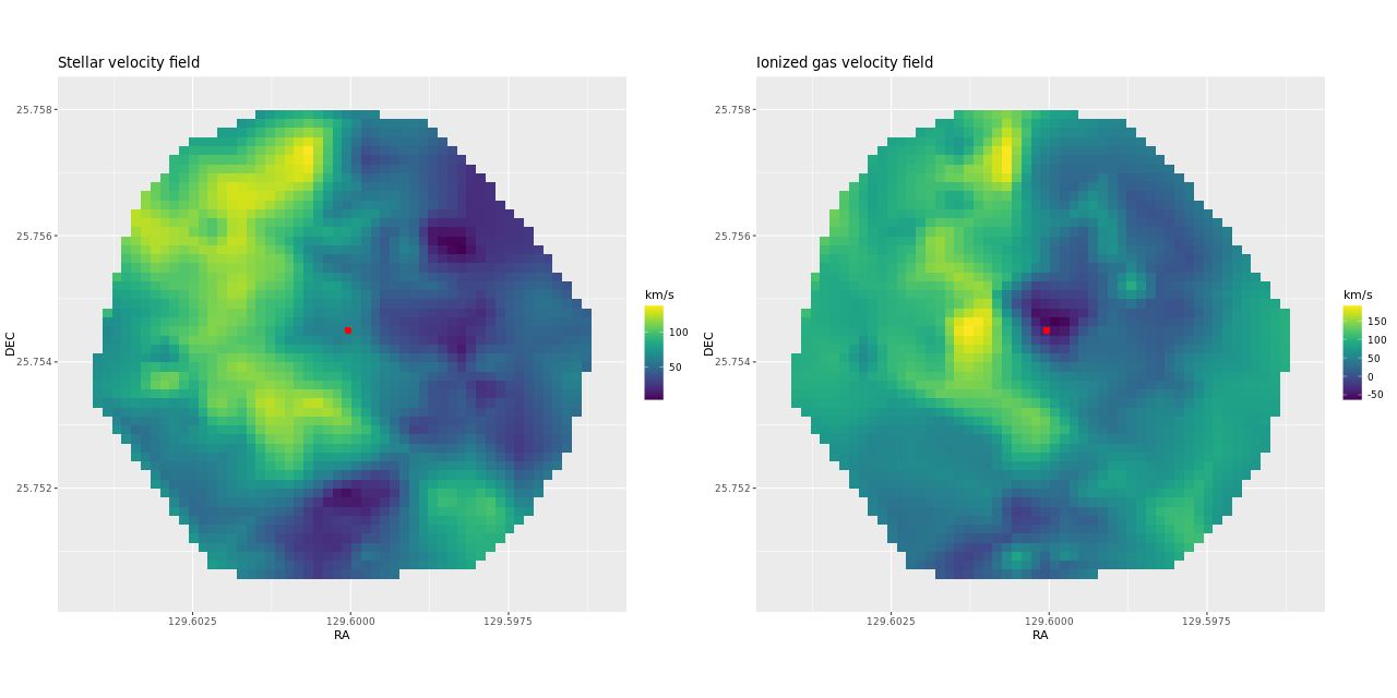
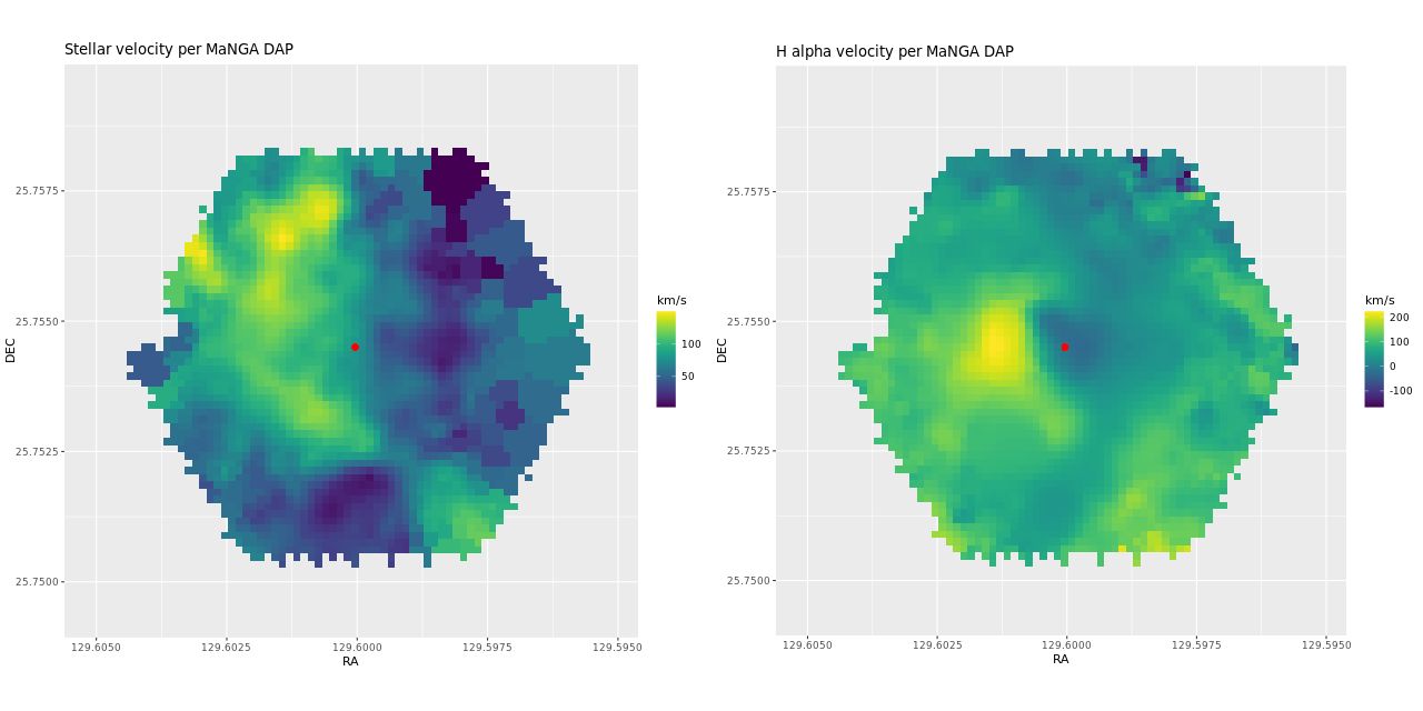
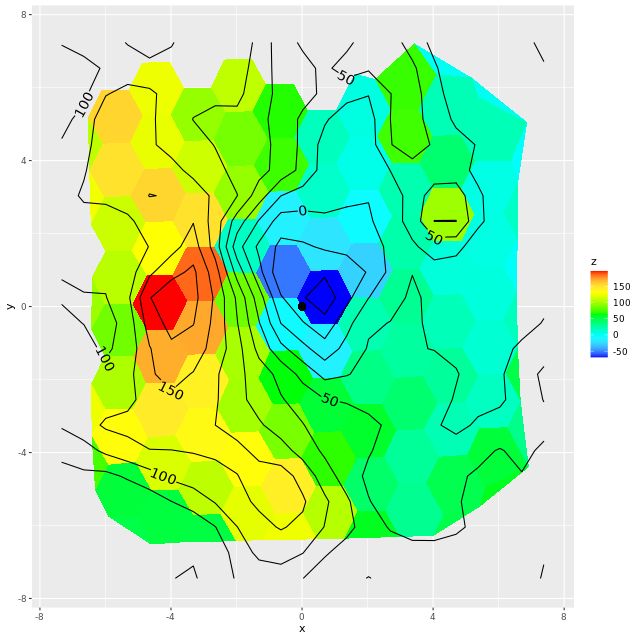
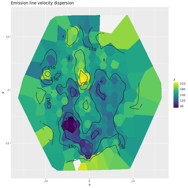
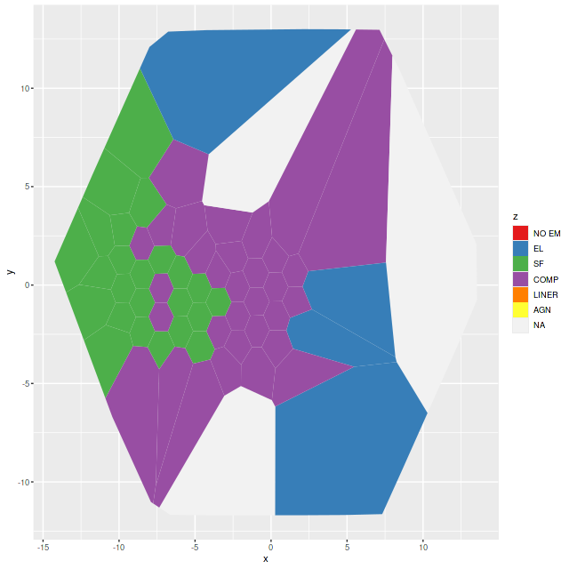
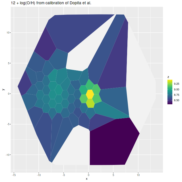
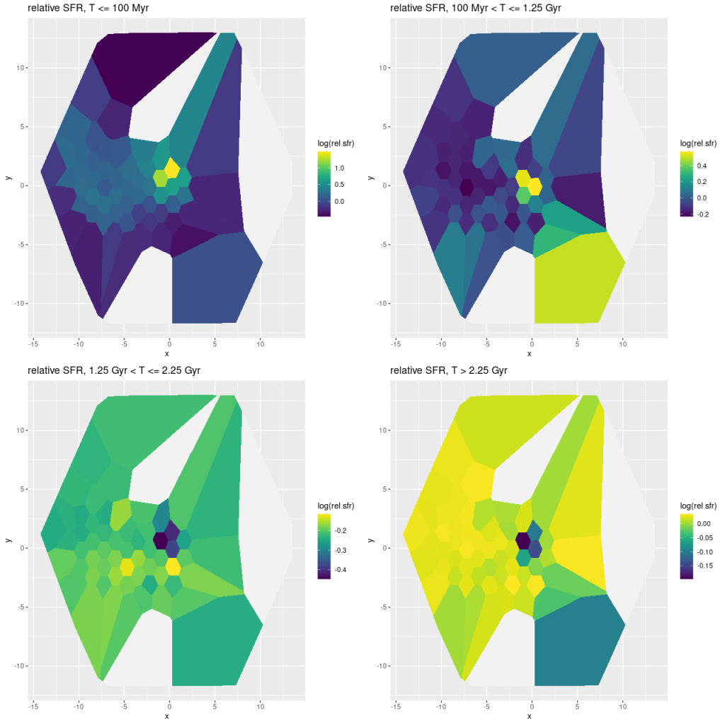
I am now, finally, going to turn to the properties of the stellar populations within the IFU footprint and detailed star formation history models. As a reminder these are based on my longstanding Stan language based code for nonparametric SFH modeling using what I refer to as the “medium” ProGeny based SSP model library as stellar inputs.
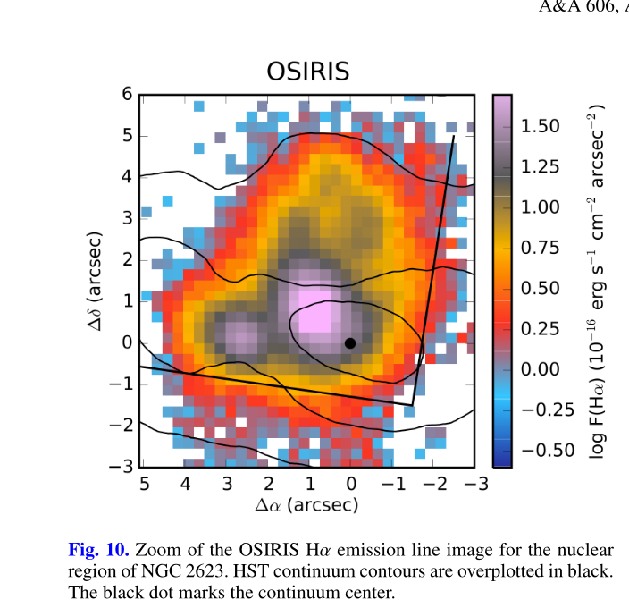
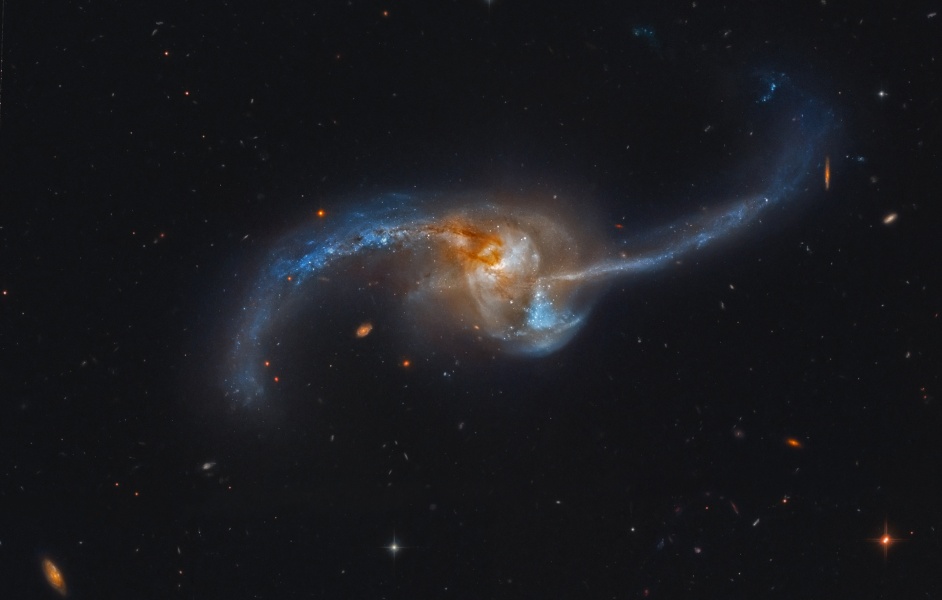
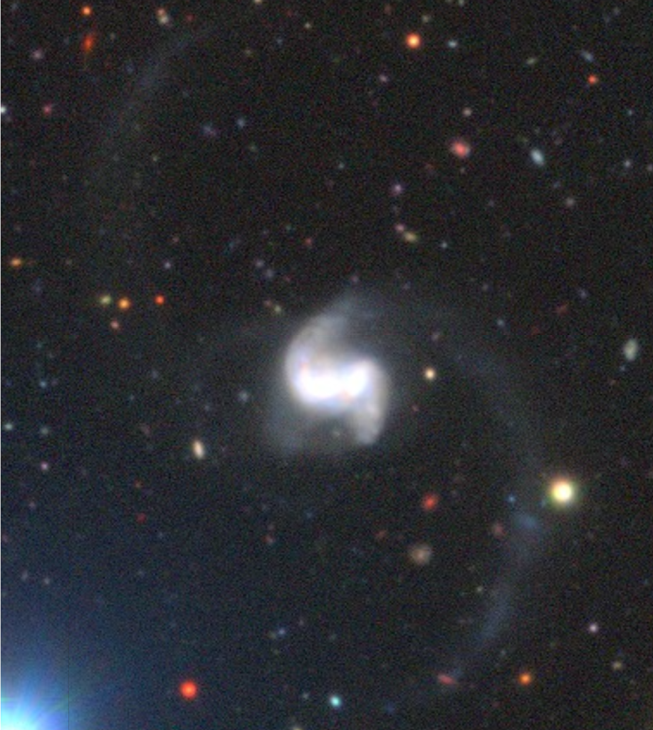
There are several distinct regions of interest, and I’ve taken the liberty of grabbing a screenshot from a figure in Cortijo-Ferrero et al. (2017) for orientation. The central region generally outlined by the Hα contour lines has the highest stellar mass density and ongoing star formation. The 3 H II regions marked C1, C2, and C3 are clearly seen in the emission line maps in my previous posts.
The wedge shaped region in the south that looks relatively blue in optical wavelength color images will turn out to be especially interesting. In the merger models of Privon, Barnes et al. (2013) the material in what Mulia, Chandar, and Whitmore (2015) call the “pie wedge” belongs to the progenitor that formed the northeastern tidal tail and constitutes the base of the tail that is now falling back into the main body of the merger remnant. As we will see the wedge contains most of the post starburst regions in the galaxy. There are also post starburst regions in a chain of bright clumps mostly west and north of the nucleus.
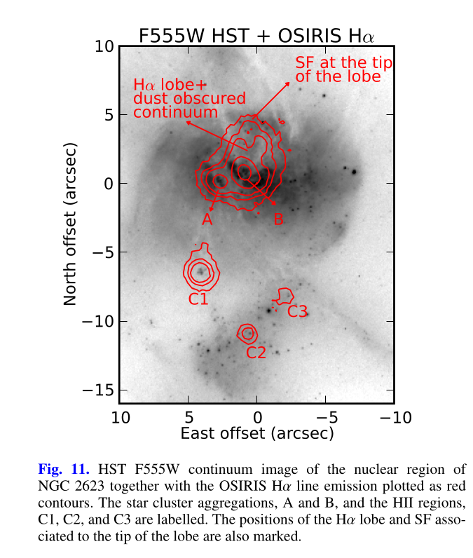
There have been a number of attempts to characterize the stellar populations of this galaxy. In a probably non-exhaustive literature review I found 4 that used HST multiband imaging and aperture photometry to estimate the ages of clusters in the tidal tails and wedge: Evans et al. 2008, the aforementioned Mulia, Chandar and Whitmore 2015, Linden et al. 2017, and Cortijo-Ferrero et al. 2017. All of these used broad band color-color diagrams and various versions of BC03 SSP models for age estimates, which is evidently not very precise and highly degenerate with dust reddening. Fortunately the pie wedge region has very low attenuation in my models (τV ≲ 0.25). Nevertheless there’s a wide range of estimates in these works. Evans estimated ages of ~1-100 Myr for clusters in the pie wedge. Mulia also found ages of ~100 Myr, claiming that much of the observed scatter was due to photometric errors. They also estimated the age of the diffuse light, finding a somewhat older age of ~500Myr. Linden et al. found a wide range of ages from 3.5-350Myr in just 11 clusters in the pie wedge and the bright clumps west of the nucleus. In an appendix to their mostly CALIFA based study Cortijo-Ferrero used archival HST images to estimate cluster ages to the south of the nucleus in the range 100-400 Myr, with an average ~250 Myr.
There have been 4 IFU based spectroscopic studies that I have found. The study by Lipari et al. that I discussed in the previous two posts exclusively considered emission line properties. Medling et al. (2014) performed a near IR study using an instrument named OSIRIS primarily directed at stellar and gas kinematics. The spatial coverage of their observations was only ~500pc, which is smaller than a MaNGA fiber so their work is not directly relevant. One interesting result is they found the nuclear stellar population to have a mean age ~30Myr.
I already mentioned the CALIFA based study of Cortijo-Ferrero et al. A second paper in the series (Cortijo-Ferrero et al. 2017) performed a comparative study of several (U)LIRGs. Their work is the most similar in objectives and to some extent methodology to mine. I’ve only found two studies concerning stellar population properties using MaNGA observations. Kauffmann et al. (2024) found strong evidence for a population of Wolf-Rayet stars in the circumnuclear region, which would prove the presence of a recent or ongoing nuclear starburst. As I mentioned a few posts ago this was a candidate “Central Post Starburst Galaxy” in the work by Leung et al. For reasons that I may get around to discussing later they chose not to analyze it as part of their final sample.
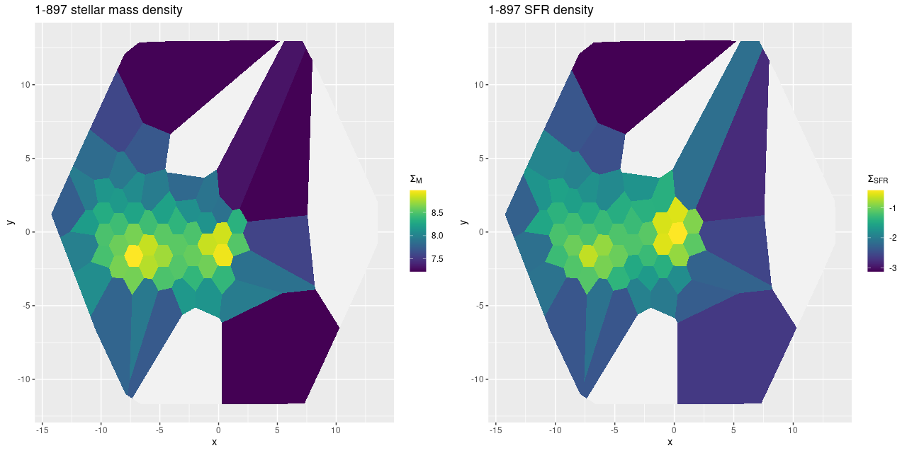
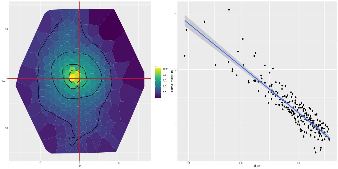
Turning to my own model results I’ll first look at some large scale properties, in no particular order. The stellar mass density peaks just to the east of the nucleus, approximately at the position of the cluster aggregation marked “A” in the HST based image above. The trend with radius appears to be close to exponential, suggesting this system is still disky.
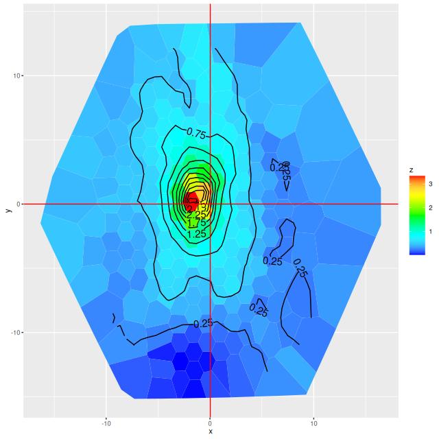
The stellar dust attenuation also peaks just east of the nucleus. Given the complex dust geometry it’s possible my simple one component attenuation model is failing here: if the light is dominated by young stars still in their “birth cocoons” and the model fits the attenuation to them it will tend to overestimate the mass in older stars. This may be a case where I’d be justified in running a model with two dust components.
In the south the area of the pie wedge has mostly very low attenuation, as do the bright clumps south and west of the nucleus.
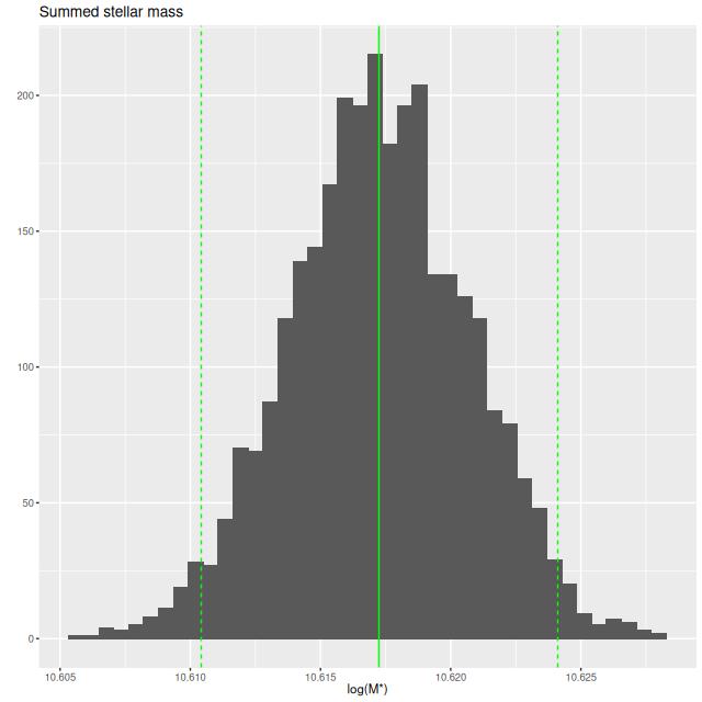
I estimate the total stellar mass within the IFU to be ≈ 4×10¹⁰ M☉ (log(M*) = 10.617 ± 0.0071which is wildly overoptimistic. This is just a sum over all individual estimates, which should overstimate the total by about 0.2 dex since the fiber positions overlap. However the IFU doesn’t quite cover the full visible extent of the main body and almost none of the tidal tails, which will add perhaps a similar amount to the total. This estimate appears within the range I’ve found in the literature. For example Shangguan et al. (2019) give an estimate of log(M*} = 10.60 ± 0.2 (for future reference they estimate the star formation rate to be log(SFR) = 1.62 ± 0.04). The previously cited Cortijo-Ferrero et al. (2017) estimate it to be 2.4 x 10¹⁰ M☉ with Chabrier IMF. Howell et al. (2010) estimated the stellar mass as 6.42×10¹⁰ M☉ (log(M*) = 10.81) and the star formation rate at 69.19 M☉/yr based on IR/UV photometry. The NASA Sloan Atlas catalog, which serves as the source for derived quantities in the MaNGA DRP estimates the stellar mass to be 3.1 – 3.4×10¹⁰ M☉.
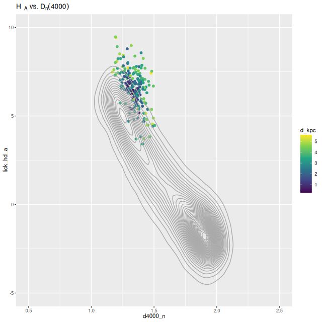
A popular absorption line diagnostic, and one I’ve displayed several times, is a plot of Balmer line strength versus the 4000Å break strength. Although it doesn’t uniquely constrain the evolutionary state of a system it does give some rough idea of the contribution of intermediate mass stars and the mean stellar population age. Plotted below are the Lick HδA index and Dn(4000). The contour lines are for a large fraction of SDSS galaxies measured by the MPA-JHU pipeline. Note that many of the points are above the last contour line in the region, which indicates a significant fraction of the galaxy is in a post-starburst state.
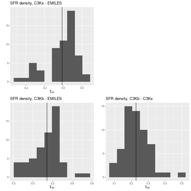
Part of my post-processing of models are calculations of star formation rate surface densities log10(ΣSFR) in units of M☉/yr/kpc2 averaged over a preselected lookback time interval. I’ve always used 100Myr as that interval, mostly because it’s a nice round number that’s often used in the literature. This time I decided to do also a calculation for a 10Myr lookback time, which is about the timescale for estimates based on Hα luminosity. The results are shown below: the top row are the estimates, and the difference is in the bottom left. As can be seen in the scatterplot at bottom right a small region near and just east of the center has had a recent increase in star formation, while it’s remained nearly constant out to about 1.5 kpc (~ 1/2 reff) and has declined farther out.
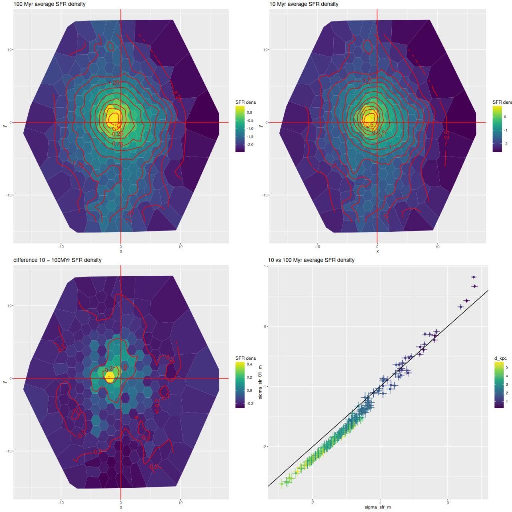
Top row – model mean star formation rate density averaged over 100 and 10 Myr intervals (logarithmically scaled). Bottom left: difference between 10 and 100 Myr averages. Bottom right: scatter plot of 10Myr SFR density vs. 100Myr.
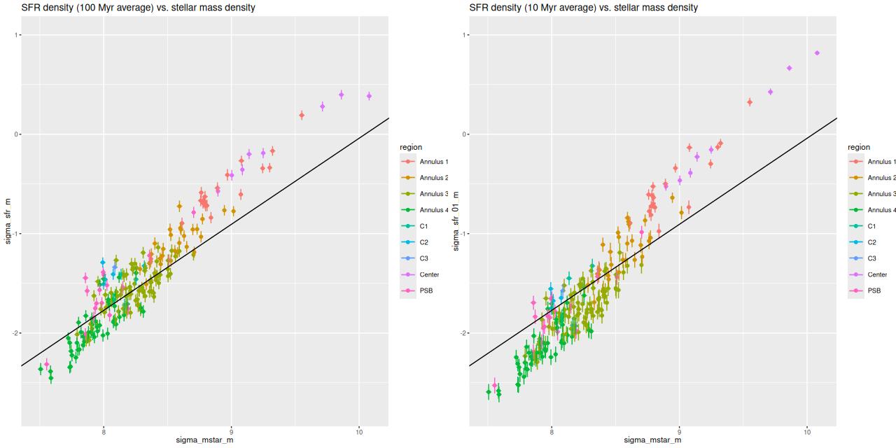
Finally, here is another standard visualization of the relation between star formation rate density and stellar mass density. The left panel is the 100 Myr averaged SFR density while the right is 10 Myr. The straight line is my estimate of the mean “spatially resolved star forming main sequence.” This was done some time ago with a sample of normal starforming disk galaxies and the EMILES + Pypopstar SSP library and should probably be recalibrated. Comparing the two plots it’s apparent that some regions are evolving into the “green valley” while others have evolved into the starbursting region.
Star formation rate histories by region
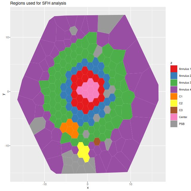
I’m now, finally, going to present detailed star formation rate histories for the entire IFU footprint. The stacked RSS spectra binned to 214 with SNR ≥ 8.5, which is a few too many to display individually. As we’ve seen there are at least 3 distinct regions with likely different recent star formation histories: the circumnuclear region has a central starburst and at least two large star cluster complexes; farther out there are 3 separate areas with star forming emission line ratios and enhanced Hα fluxes relative to their surroundings; the “pie wedge” has many star clusters with estimated ages ~100Myr and post-starburst spectra. Some of the bright clumps seen to the west of the nucleus also have post-starburst spectra. For display purposes I’ve made a slightly finer grade division as follows:
- Center region: the closest fiber to the center and its immediate neighbors including cluster aggregation “A” to the east. (see top of post). This covers most of the region with highest emission line flux.
- Annulus 1: regions with D ≤ 0,5 reff (I adopted reff = 7.9″ ≈ 2.9 kpc from the NSA atlas) and outside the center region.
- Annulus 2: 0.5reff < D ≤ 0,75 reff, excluding regions with post-starburst spectra.
- Annulus 3: 0.75reff < D ≤ 1.25 reff, excluding regions with post-starburst or starforming spectra.
- Annulus 4: D > 1.25 reff, excluding regions with post-starburst or starforming spectra. The maximum IFU coverage is 2reff.
- I chose to display the 3 regions of H II aggregations separately. The first is the one labelled “C1” in the graphic at the top of the post.
- H II region(s) “C2”
- H II region(s) “C3”. Both of these lie at the edge of the “pie wedge.”
- Visual examination of the spectra showed that many of them have classic A+K like spectra, with very strong Balmer absorption and weak emission (this was known some years ago: see Liu and Kennicutt 1995). I made a PSB region selection with highly stringent criteria:
- Lick HδA – 2σ(HδA) ≥ 6.25Å
- BPT class of “EL” or “NO EM” (i.e. weak or no emission lines detected). I used this instead of the more traditional equivalent width criterion mostly because I haven’t validated my EW calculations.
Essentially all of the “pie wedge” meets these criteria, as do several bright clumps west of the nuclear region. With relaxed selection criteria much of the galaxy outside the circumnuclear region could qualify by, for example Alatalo‘s criteria for “Shocked POststarburst Galaxies.”
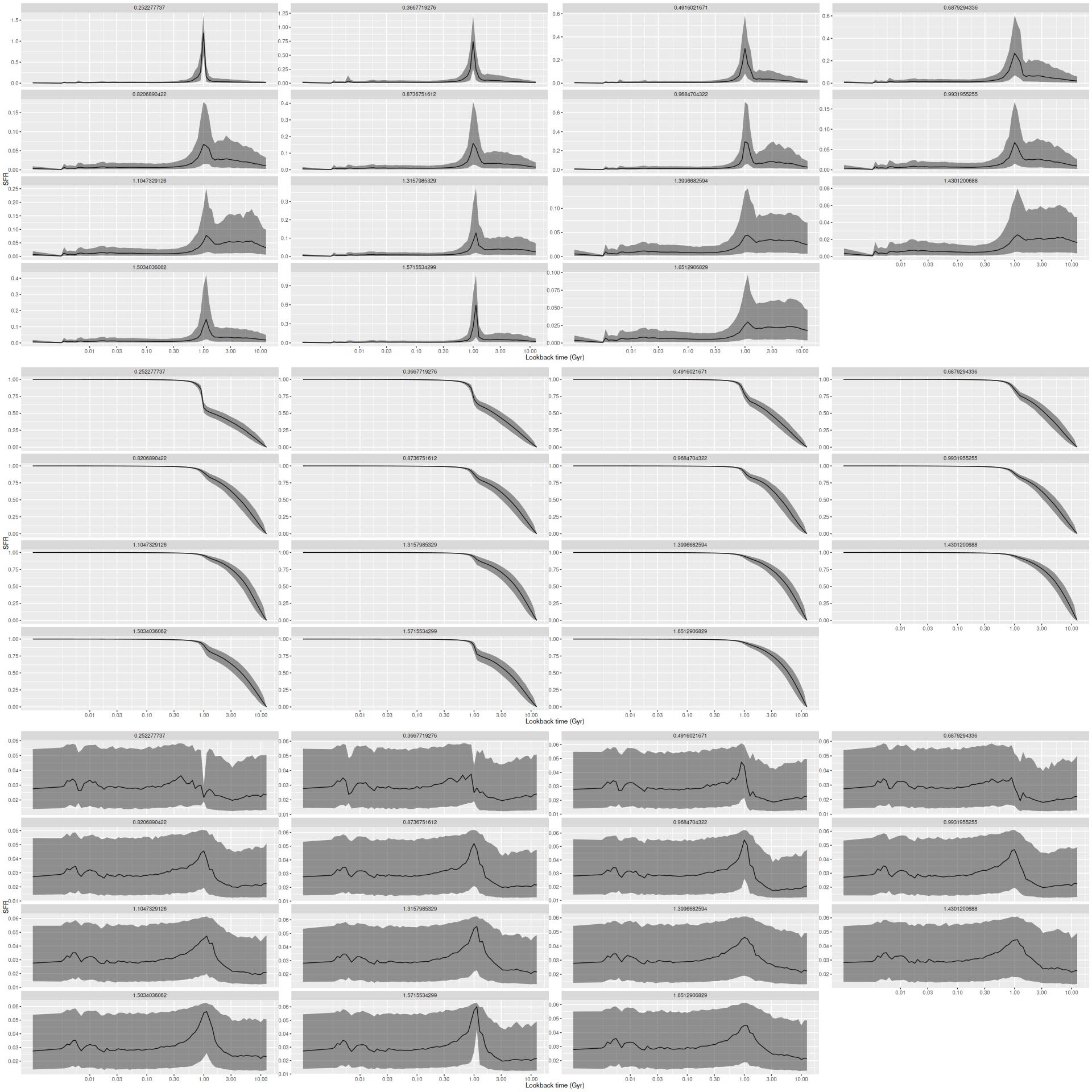
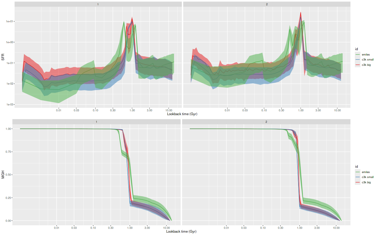
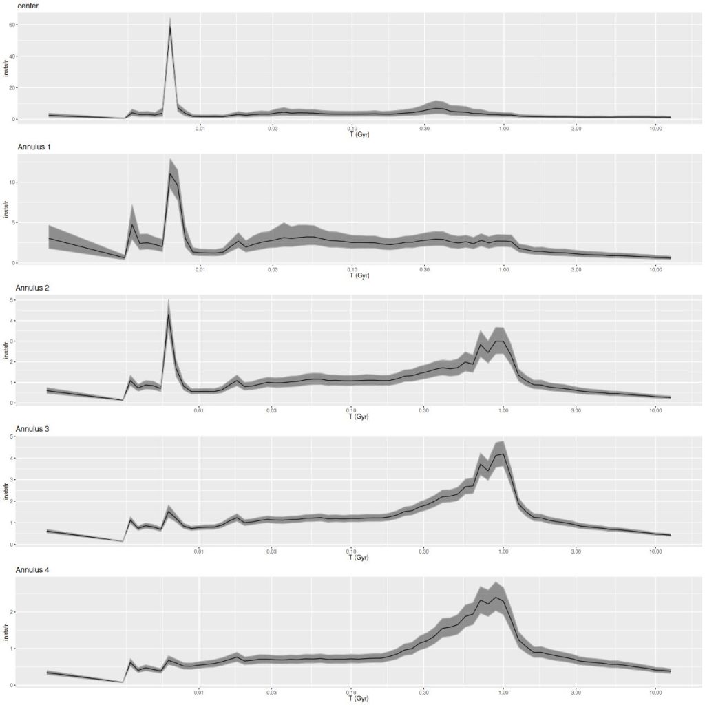
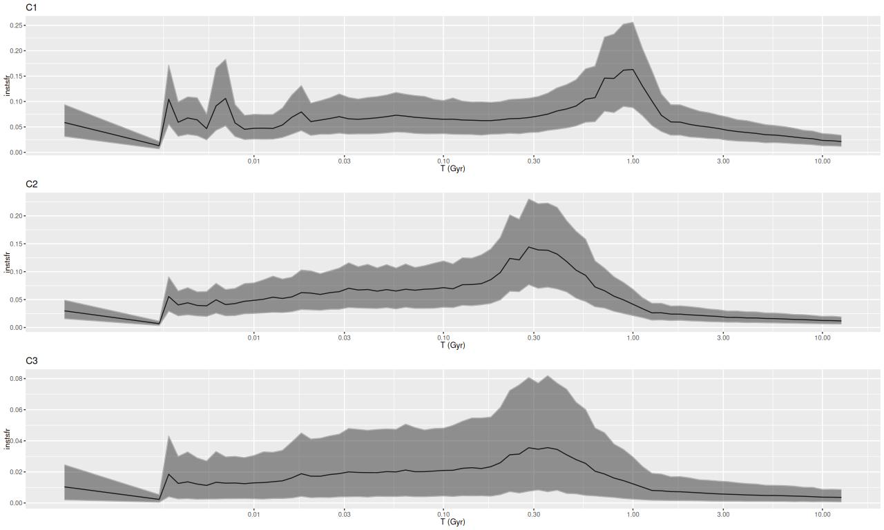
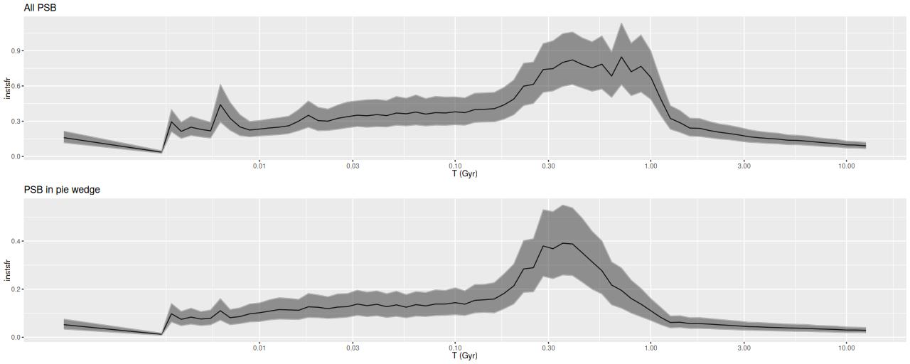
Modeled SFR histories are shown below grouped into 3 sets. The horizontal axes are logarithmically scaled, while the vertical axes are linear with different scales for each plot. Units are M☉/yr; these are estimated by summing over all models for the binned spectra comprising each group.
SFH in annuli
Star forming regions
Post starburst regions and the “pie wedge”

To summarize my visual impressions, star forming appears to have accelerated beginning ≈1 Gyr ago. In what is now the main body of the galaxy it plateaued shortly thereafter and then slowly decayed until very recently (< 10 Myr) where we are seeing a centrally concentrated starburst with declining star formation in the outskirts of the main body.
In the pie wedge including the two starforming regions the peak was much later at ≈300 Myr, and again with a subsequent slow decay. The only difference between the starforming and PSB regions of the wedge is the former evidently still have enough residual star formation to power H II regions. The PSB regions outside the pie wedge have a much different SF history from those inside it, with an early peak at ~1 Gyr and slow decay, much like the rest of the galaxy outside the center. The broad plateau in the first of the PSB plots is therefore a bit of an illusion.
Although it’s obscured by the current starburst the central region also had a peak at ≈300 Myr.
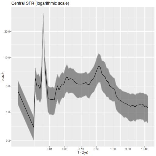
The 300 Myr peak is consistent with Privon et al.’s estimate of a first pericenter passage at ~220 Myr ago as well as the HST based estimates of star cluster ages in the wedge. However coalescence at ~85 Myr ago seems to have had no effect on star formation in my models — this is in contrast to most recent merger simulations, which typically have a strong centrally concentrated starburst around the time of coalescence. The large scale enhancement of SFR beginning at ~1 Gyr is also a bit puzzling. If the model is correct the effects of the interaction began well before the merger was underway.
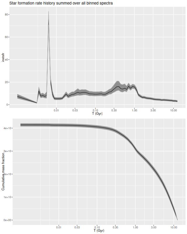
Finally for this section, here is the model star formation history summed over all 214 individual models. System wide there was a broad plateau from ~! Gyr to ~300 Myr ago, with a slow decline until ~10 Myr. The recent starburst only adds about 0.3% to the present day stellar mass, ~108 M☉.
Selected individual SFH models
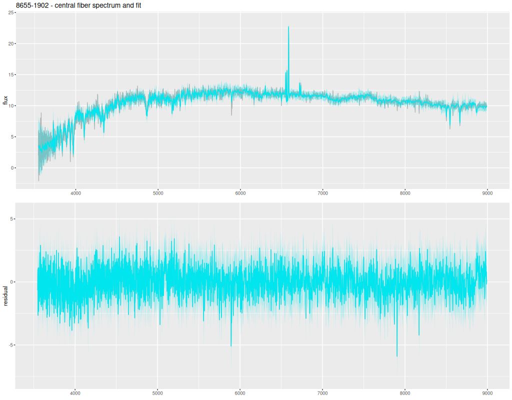
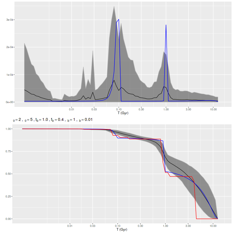
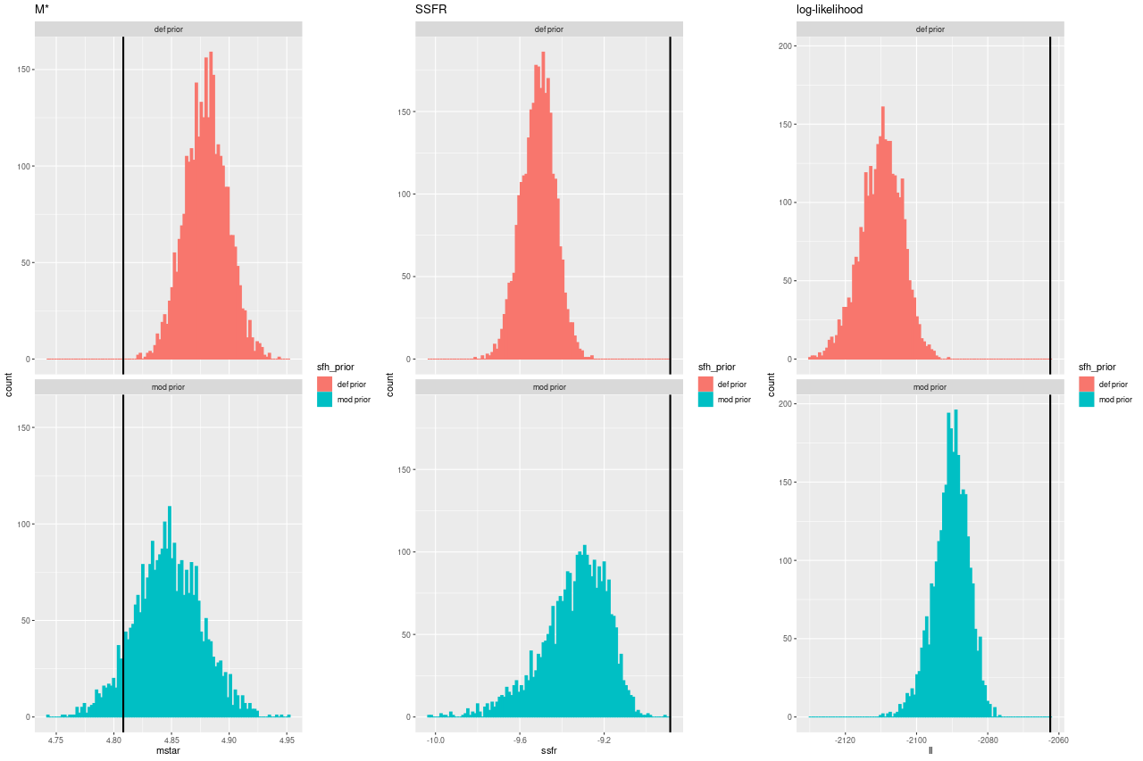
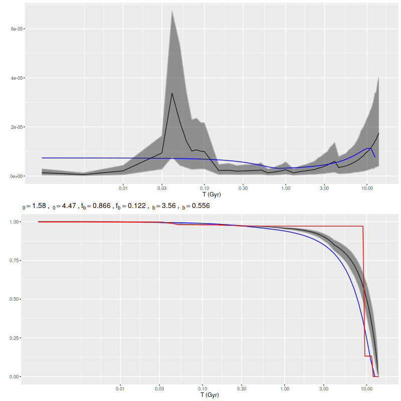
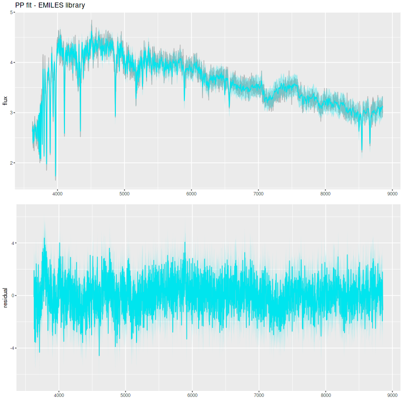
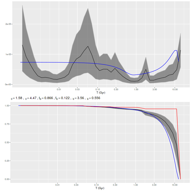
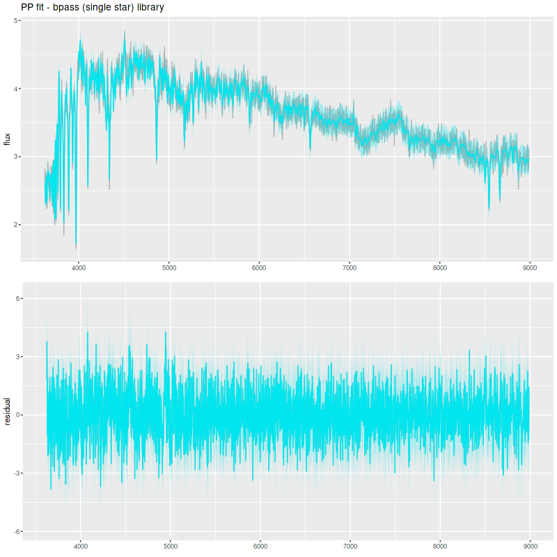
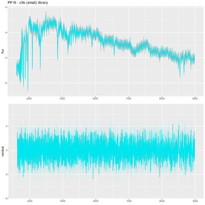
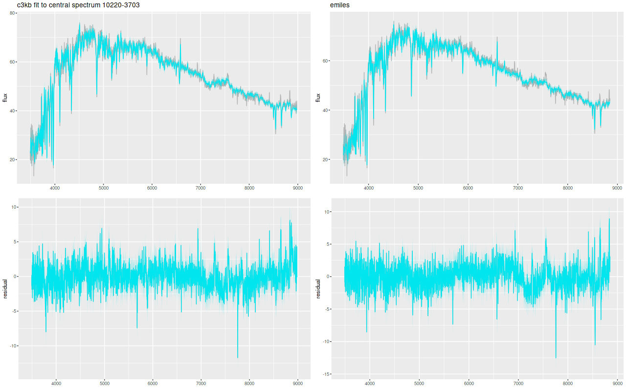
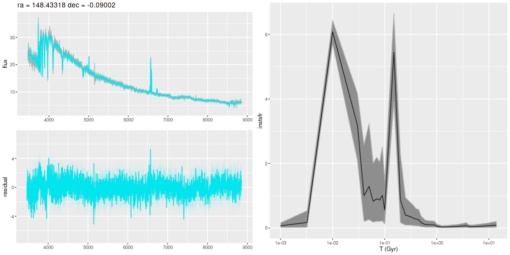
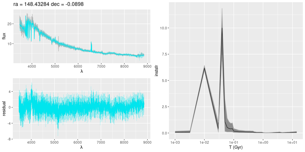
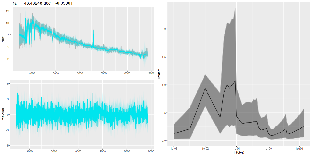
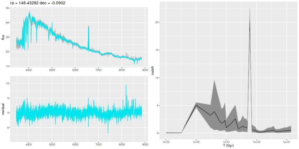
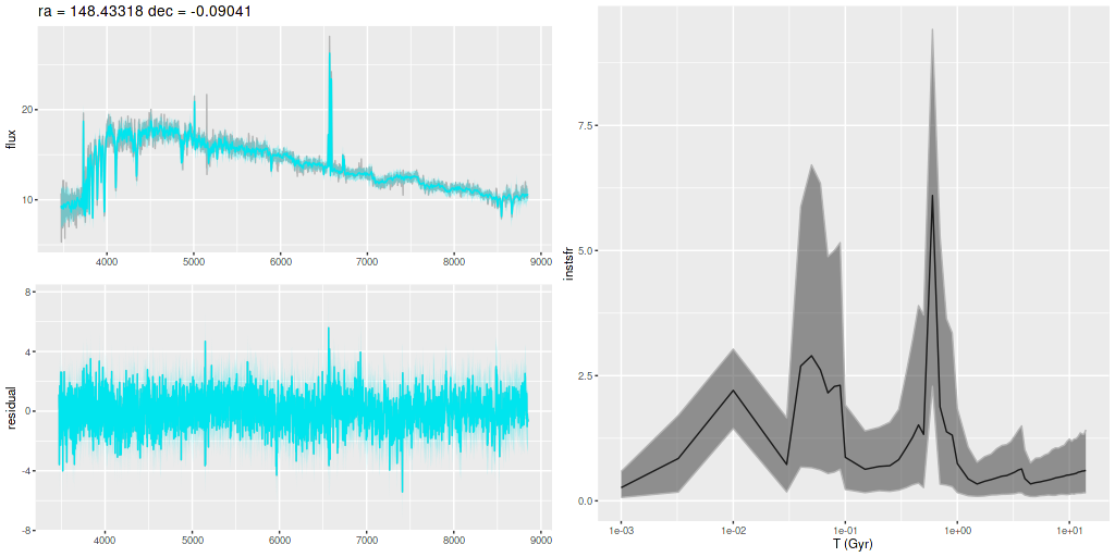
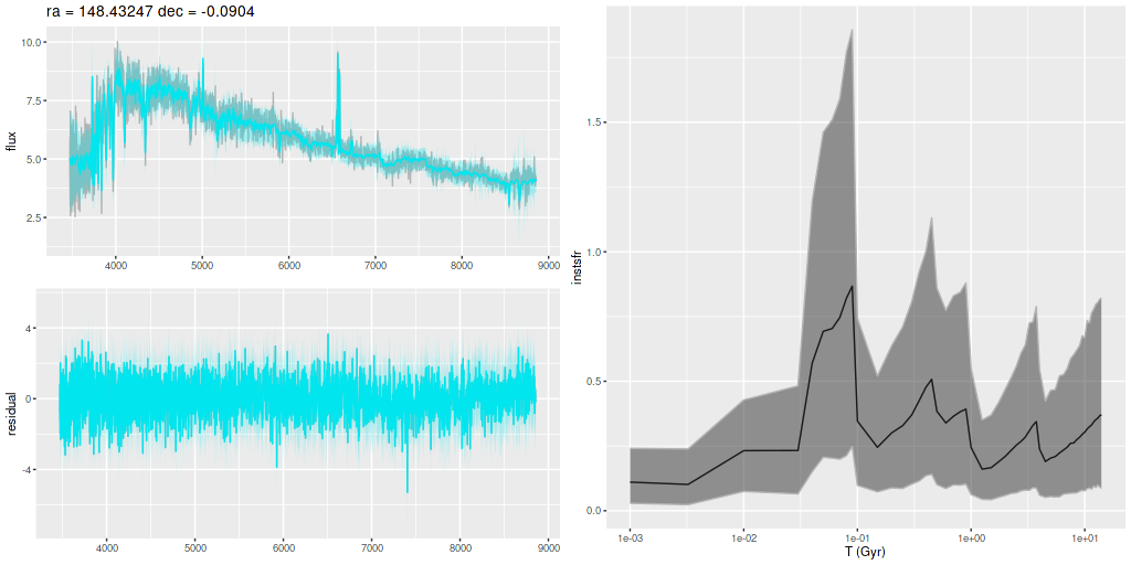
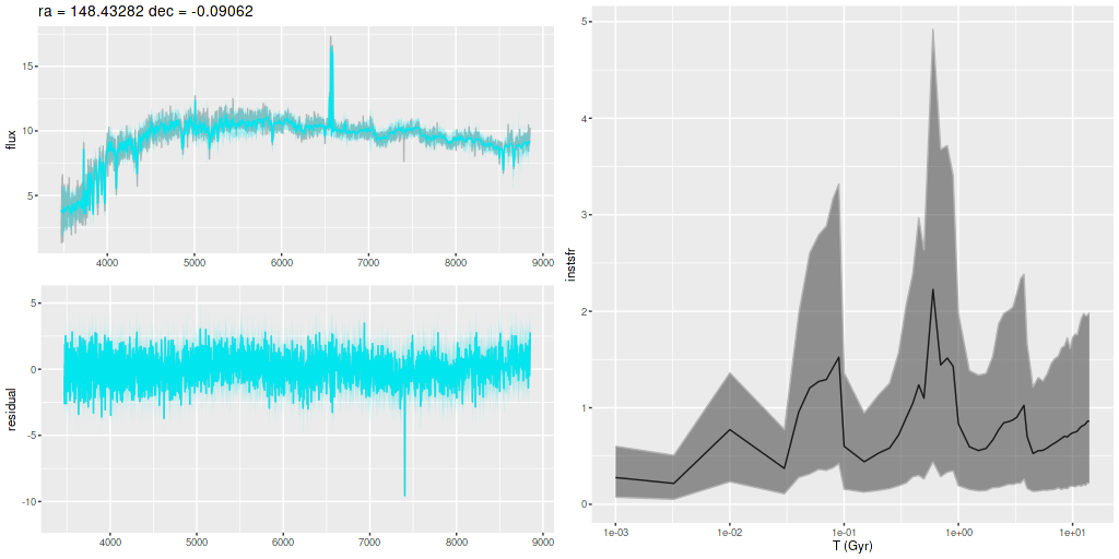
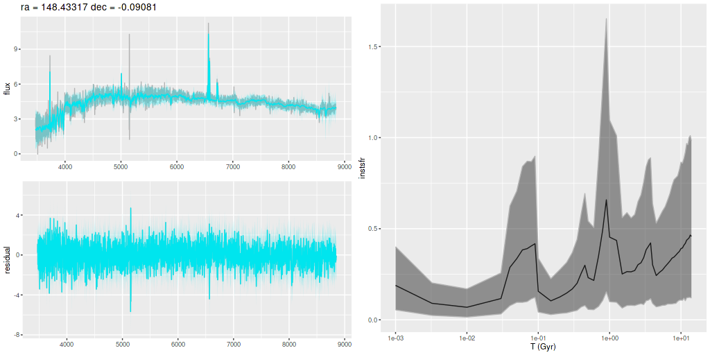
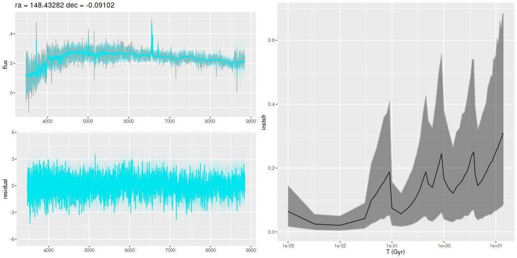
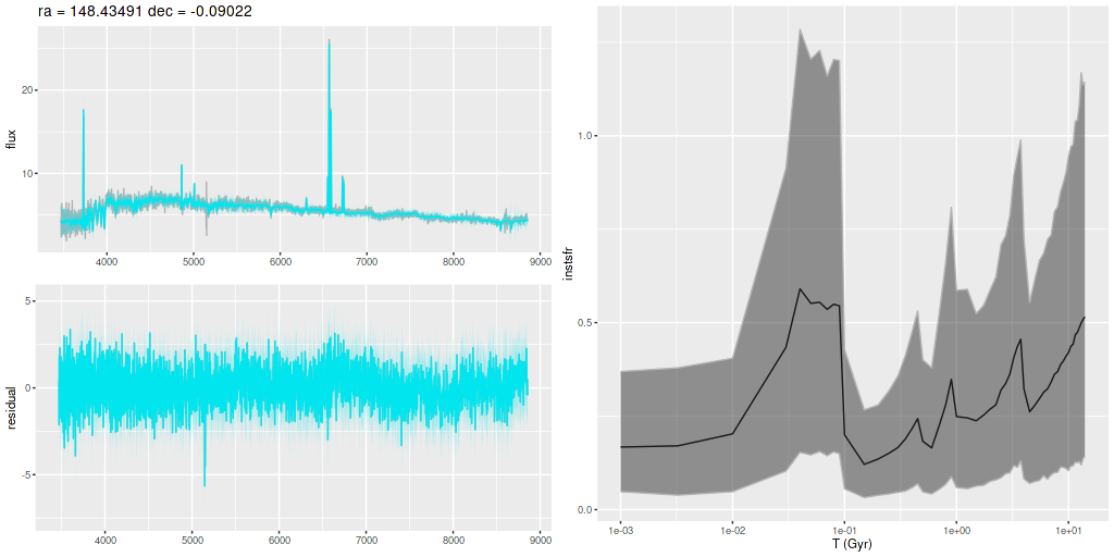
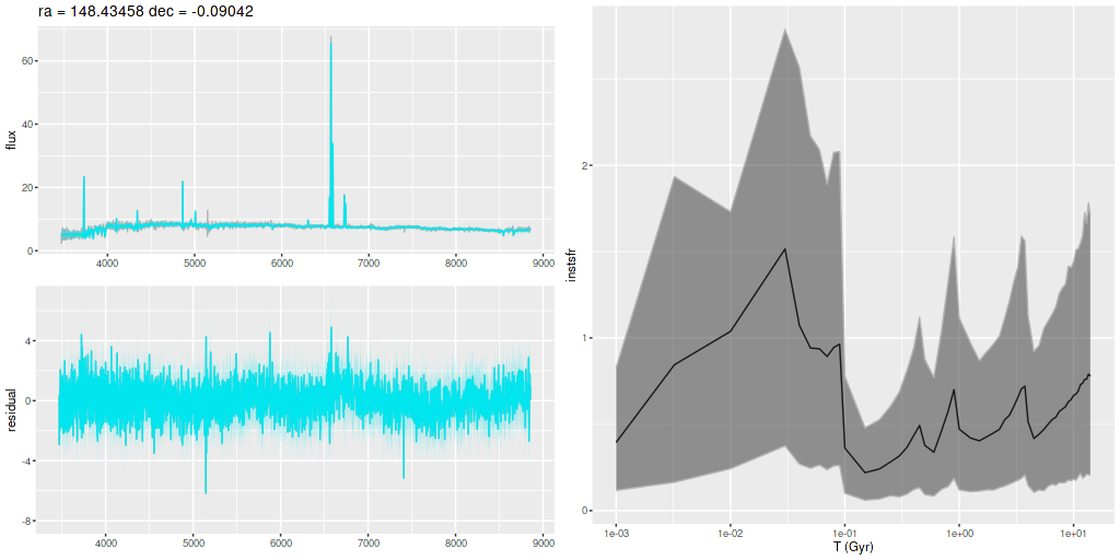
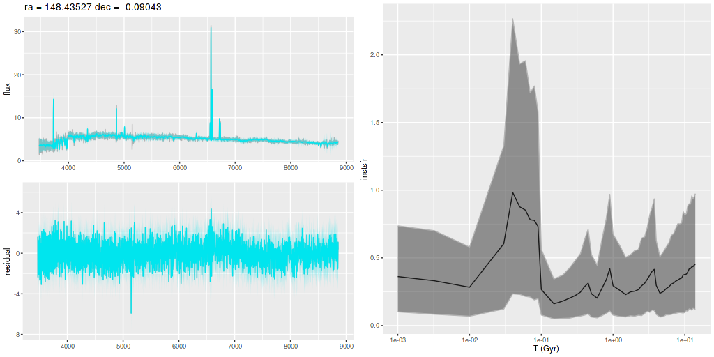
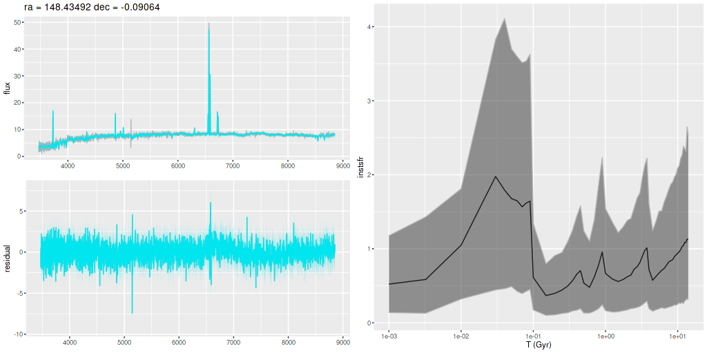
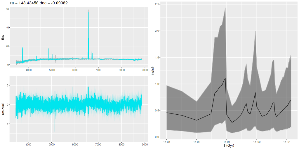
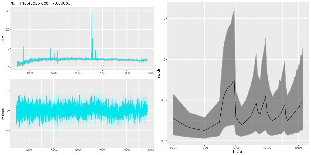
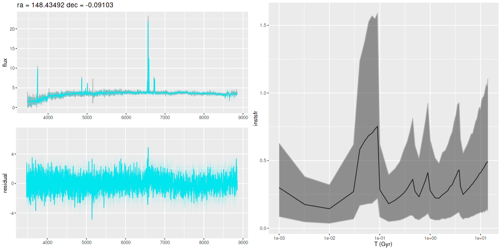
Plotted below are model star formation histories and fits to the data for 13 individual spectra, with the same ordering by region as the previous subsection. All horizontal scales are the same: lookback times are logarithmically scaled in Gyr; wavelengths are rest frame and cover the range of the model fits, which is ≈3560-9000Å. Vertical scales are linear with ranges chosen to cover the values plotted in each model run. The SFH plots include the position of the fiber center.
I picked four regions from the center. First is the fiber closest to the nucleus. One oddity of the RSS files is the central fiber is usually offset from the IFU center, in this case by about 3/4″ to the NW. The IFU center is exactly at the consensus position of the nucleus, and there are two fibers that straddle it. The other one is located just to the SE– notice that it has a much higher peak star formation rate than its immediate neighbor and a considerably redder continuum. The region with the highest 100 Myr average star formation rate is the neighbor to the NE, which is close to the cluster aggregation “B” in the HST image at the top of this post. Finally for the center spectra, the highest 10 Myr averaged SFR density of ≈7 M☉/yr/kpc2 is the region to the east that is centered in a prominent dust lane and includes at least part of cluster complex “A”. It also has the highest model stellar attenuation (τV≈3.3) and the highest Hα luminosity density corrected for stellar attenuation.
Fits to the data are somewhat problematic in the center. The non-Gaussian emission line profiles are prominent in the residuals. and there are systematic residuals in the stellar continuum as well. The complex dust geometry and kinematic decoupling of gas and stars are likely contributors to the lack of fit, and there are the usual issues of possibly missing ingredients in the inputs. How much the fit errors affect the SFH models is unknown.
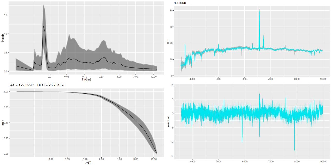
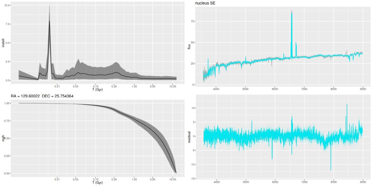
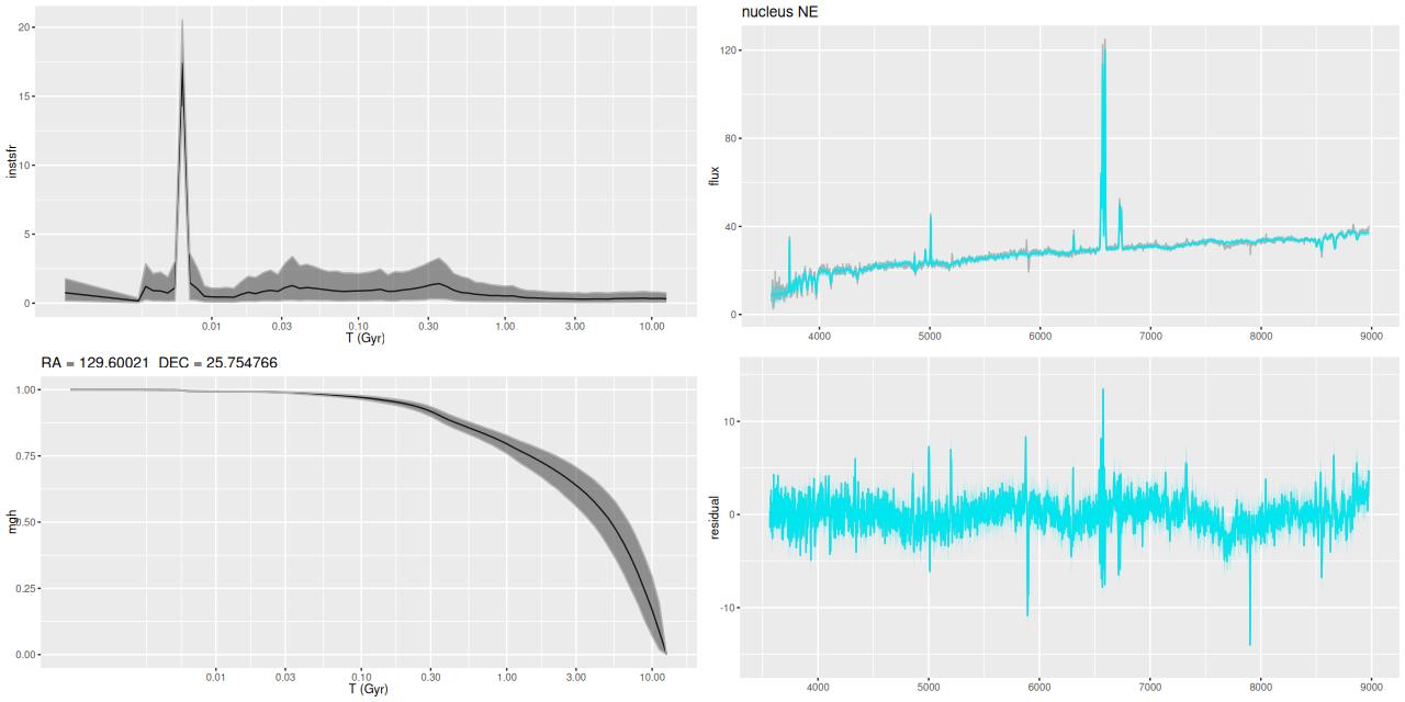
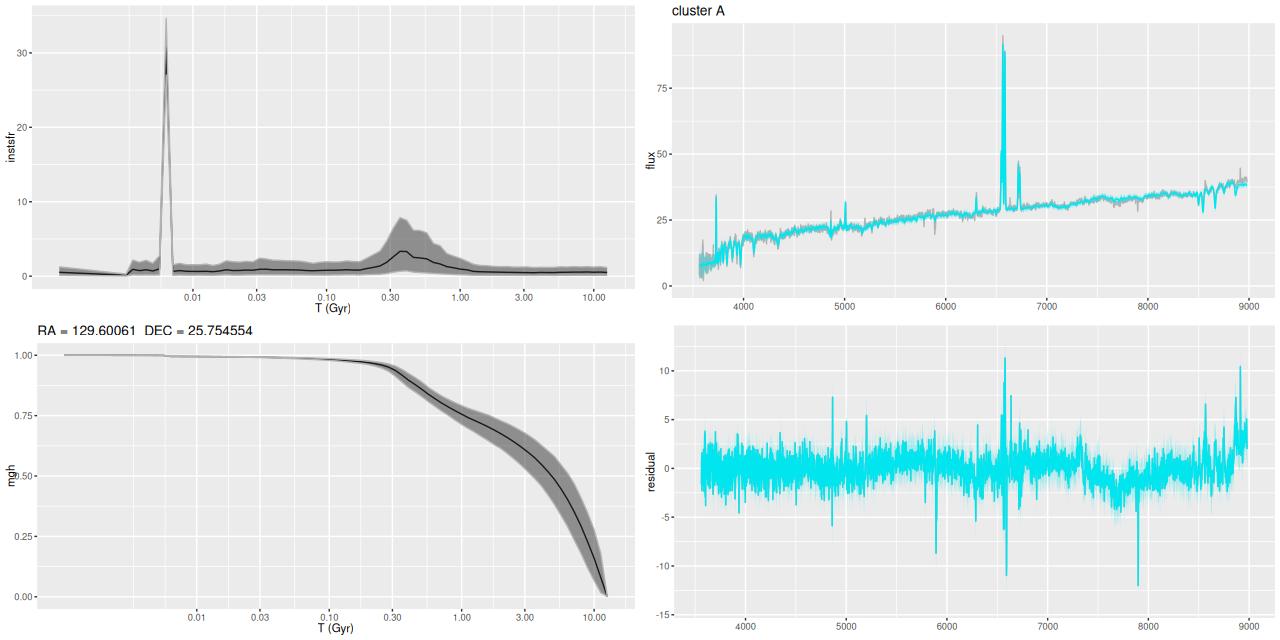
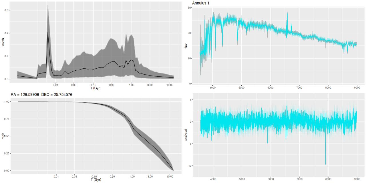
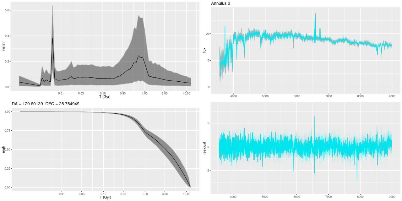
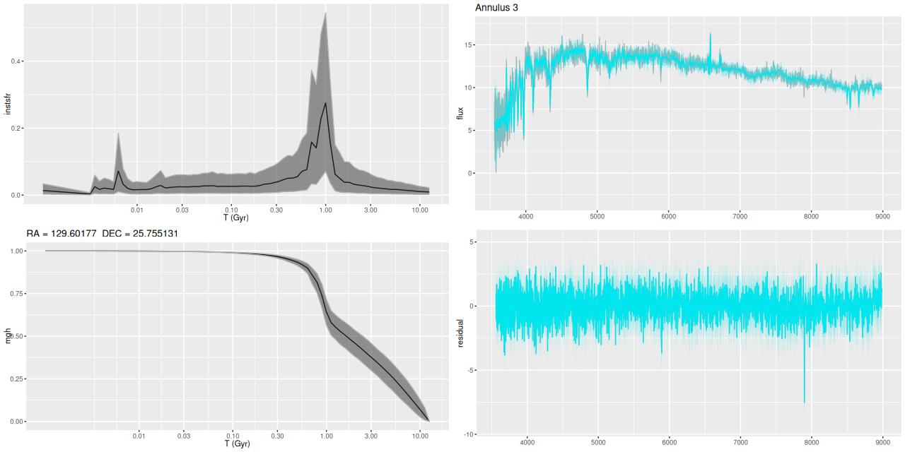
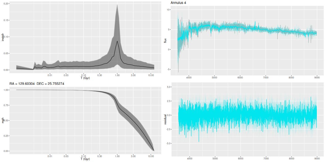
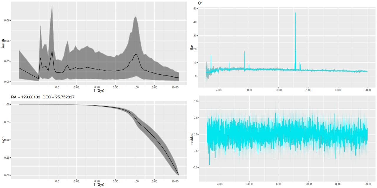
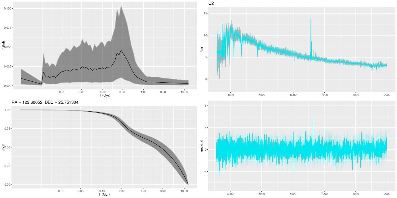
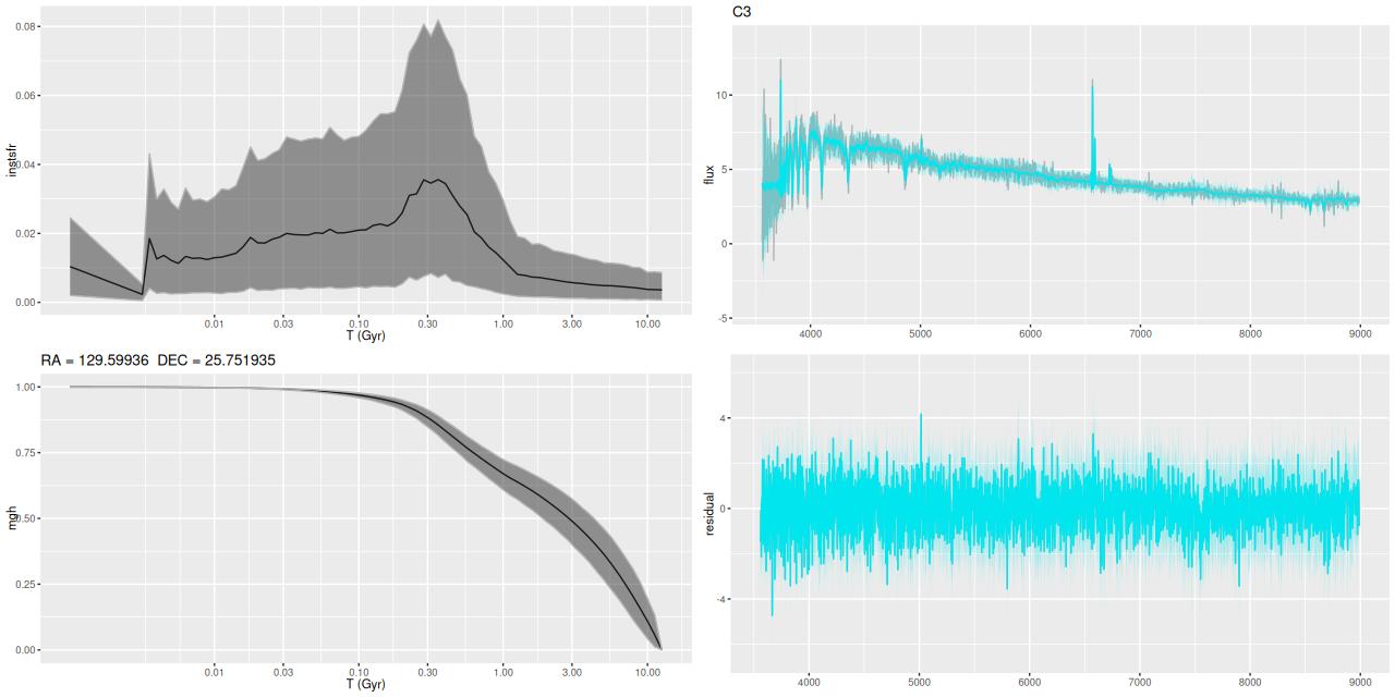
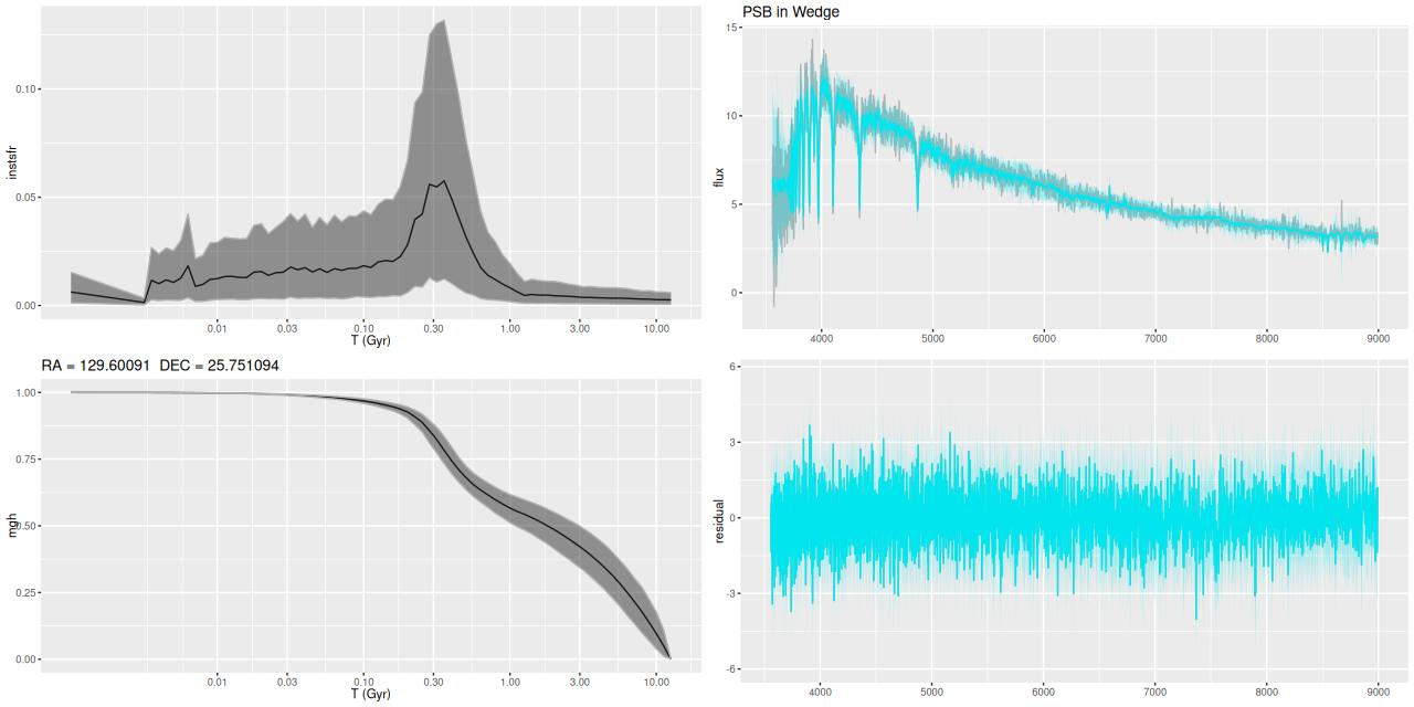
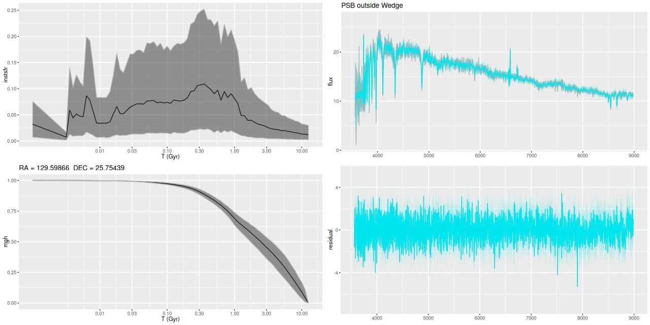
Sample star formation histories and posterior predictive fits to the spectra. Fiber center position and galaxy region are indicated on left and right panels respectively
A brief comparison with Cortijo-Ferrero
As I mentioned previously Cortijo-Ferrero (2017a, 2017b) published two papers studying this galaxy and a small number of other (U)LIRGS using data from CALIFA and a few other instruments. Their objectives in paper (a) were essentially the same as mine in these posts, and their methods were somewhat similar. For spectral fitting they used a code named STARLIGHT, which is not Bayesian and as far as I can tell doesn’t have any convergence guarantees but does perform nonparametric SFH modeling.
The first paper devotes one section apiece to ionized gas properties and stellar populations. Since I’ve discussed the former at some length in my previous posts I won’t review their results in detail. Quantities that I was able to compare agree well. They also found the kinematic center of the gas to be offset 2″ to the east of the nucleus, in agreement with my results and Lipari. They comment that the offset is “within (their) spatial resolution,” which is true but misses the point that the entire rotating structure is much larger and is clearly offset from the nucleus even on visual inspection.
For comparison purposes I’m going to reproduce some of their graphical results. They have maps of many quantities as well but visual comparisons are difficult because they are displayed at postage stamp size in the online journal papers and also because the authors made some truly atrocious choices of color palettes. I’ve already displayed a map of stellar mass surface density and its trend with radius, which can be compared to their figure 4 in paper (a). The values and trends with radius are similar in my models to theirs although I don’t see a break in the relation as shown in their lower plot.
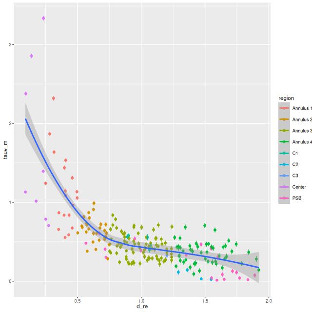
Their model for stellar dust attenuation is similar to mine: they assume a single foreground screen with Calzetti attenuation. I include an additional parameter controlling the overall steepness of the attenuation curve, which essentially amounts to allowing RV to be variable. The peak values near the center are considerably higher in my models than theirs (cf figure 5 in paper a). This could be partly due to the slightly higher spatial resolution in MaNGA. More importantly perhaps my models have a “greyer” attenuation curve than Calzetti’s in the center which means a larger attenuation value is required for a given amount of reddening. Farther out there is good agreement.
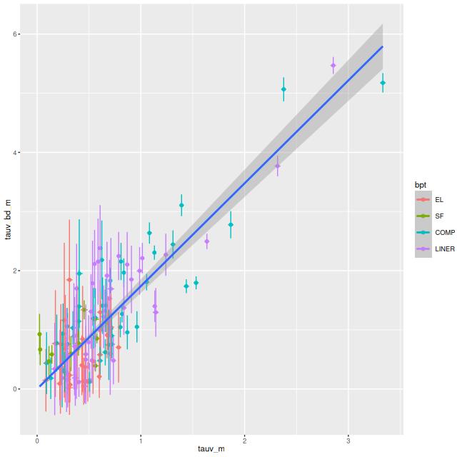
As a bit of an aside, my standard postprocessing includes estimates of dust attenuation of ionized gas using the Balmer decrement method with an assumed intrinsic ratio of Hα/Hβ = 2.86. Keeping only spectra with 3σ detections in both I get the following relation between gas and stellar attenuation. The slope of the straight line from a simple linear regression is 1.74 ± 0.06 (1 σ), which is consistent with their results (section 4.3) and, I think, other literature sources.
For reasons that escape me in paper (a) they chose to examine stellar population ages in 3 broad ranges: young (t ≤ 140 Myr), intermediate (140 Myr < t ≤ 1.4 Gyr), and old (t > 1.4 Gyr). I have a routine to calculate mass fractions in arbitrary age ranges, so I reproduce their figure 8:
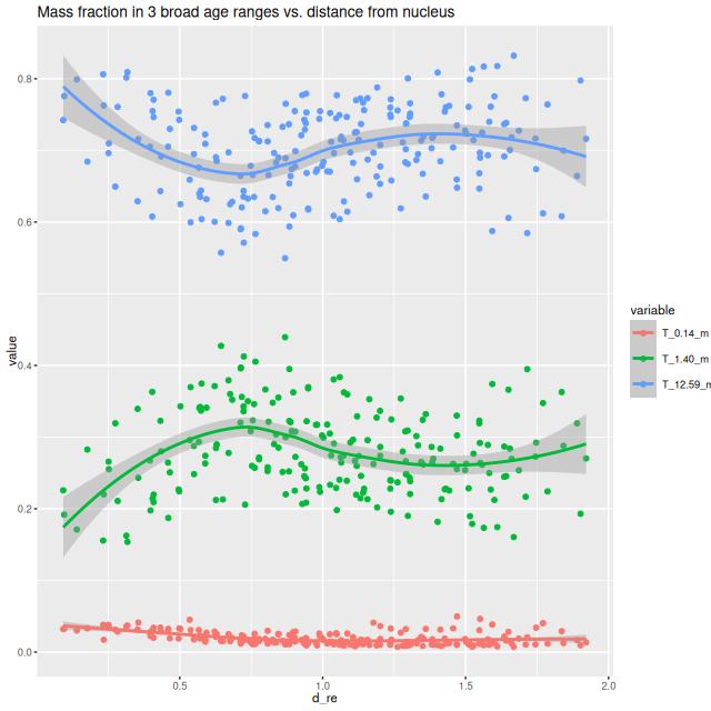
In contrast to their result there is no location where there is as much mass in “intermediate” age stars as “old” ones. However, and in agreement with them, if the SFR were constant over cosmic history there should only be about 10-11% of the total mass in young and intermediate age stars, suggesting an enhancement in SFR of a factor of ~2-3 over the past ~Gyr.
I calculated the total (IFU wide) star formation rate by summing over all individual models. The histograms below are for 100 and 10 Myr time spans: the estimated SFR has actually increased, from ≈ 10.4 M☉/yr to 13 M☉/yr in the last 10 Myr, with nominal uncertainties of ±0.5. This is entirely driven by a recent increase in the near-nuclear SFR.
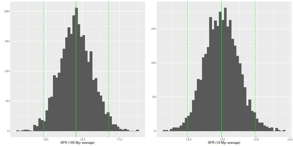
SFR estimates based on infrared data tend, understandably, to be higher — the literature sources I noted at the top gave estimates of 40-70 M☉/yr. Cortijo-Ferrero give estimates of ~8-12 M☉/yr depending on time span considered.
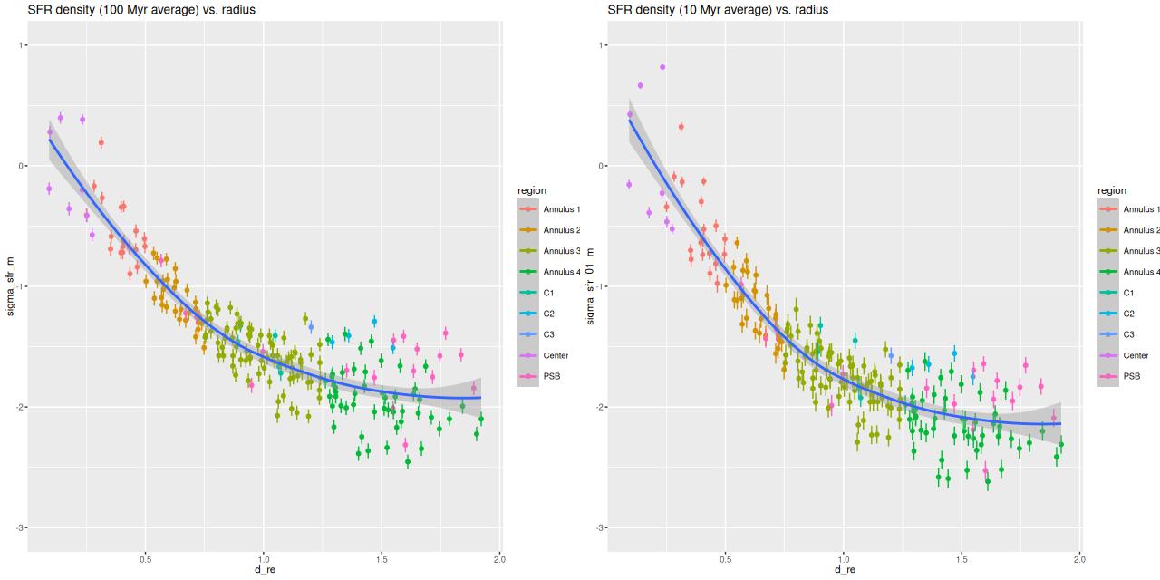
Paper (b) chose a different set of age ranges to focus on: 30, 300, and 1000 Myr, although they only discussed 300 Myr averaged star formation briefly. Instead of trying to reproduce their results for those SF timescales I’ll just show SFR density vs. radius for the 100 and 10 Myr lookback times that I’ve examined in this post. These can be compared to their figures 5 and 6. My 10 Myr plot for SFR density2add 3 to the log SFR density values to convert to the same units. looks similar to their 30 Myr except the peak values in the center are higher. In my models this is because the center has just turned on in the last <10 Myr.
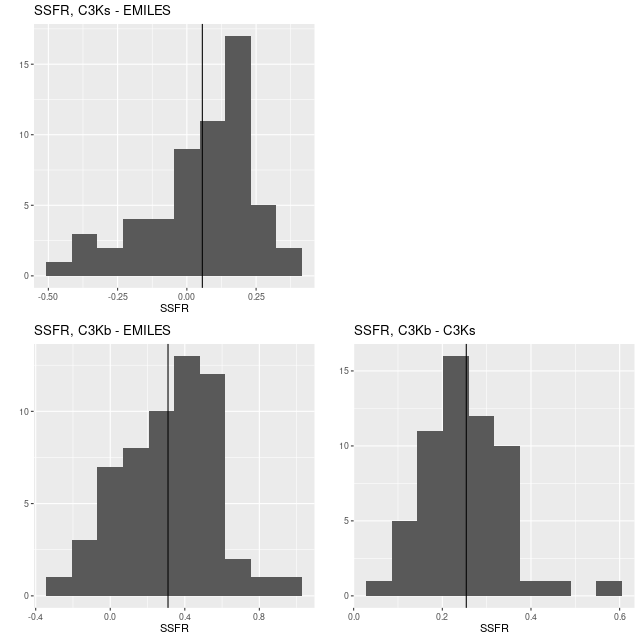
My sSFR plots don’t resemble theirs (figure 6) very closely. Both have a negative gradient within 1 half light radius while theirs have very shallow gradients. The steeper gradient in the 10 Myr plot is due to the recent central starburst and the slow decline of star formation outside the central few kpc.
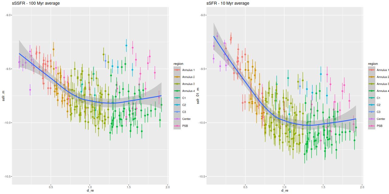
Specific star formation rate vs. radius in 100 and 10 Myr time interval. Units are yr-1, logarithmically scaled.
Looking back at the SFH plots by region, there appear to be 3 epochs of accelerated star formation. The oldest begins at ~1 Gyr, the second at ~300 Myr, and finally there is a central starburst with age ≲10 Myr. Privon’s merger simulation, which is the only source for this system, places the first pericenter passage at ~220 Myr lookback time Without knowing what level of accuracy to expect from this kind of simulation this appears to be excellent agreement, so we can confidently associate the “pie wedge” with this event, as well as the enhancement in SFR at about the same age in the very center.
What’s more puzzling is the apparent increase in SFR long before the final stages of the merger. In most recent high resolution simulations that I’ve seen SFR increases above baseline only shortly before first pericenter passage (e.g. Renaud et al. 2014).
Slightly puzzling also is that if coalescence occurred ~85 Myr ago as in Privon’s simulation there is no trace of its effect in my models. The current central starburst must have been delayed considerably compared to the predicted almost immediate starburst in recent simulations.
This is one of about 10% of candidate PSBs in the Leung et al. sample that was rejected for further analysis based on fitting issues. Oddly, this was classified as a Central PSB, which is clearly wrong (and which a cursory literature search would confirm). Their fitting issues may have arisen from their strategy of binning all spectra meeting their PSB criteria into a single one. This can’t work when physical conditions, particularly dust attenuation, vary rapidly.
I have recently, after several months of leisurely computing, completed model runs for all 91 data sets in this sample. A detailed analysis is some ways off. I need to go through each model run — some had very poor fits, possible calibration errors, or low S/N data.
