
A few brief comments about the simulations, of which I’ve done a few more but will probably bring to an end. First, here is a plot I mentioned but didn’t display last time of the bias in stellar mass estimate against the lookback time to the burst. Points are color coded by burst strength.
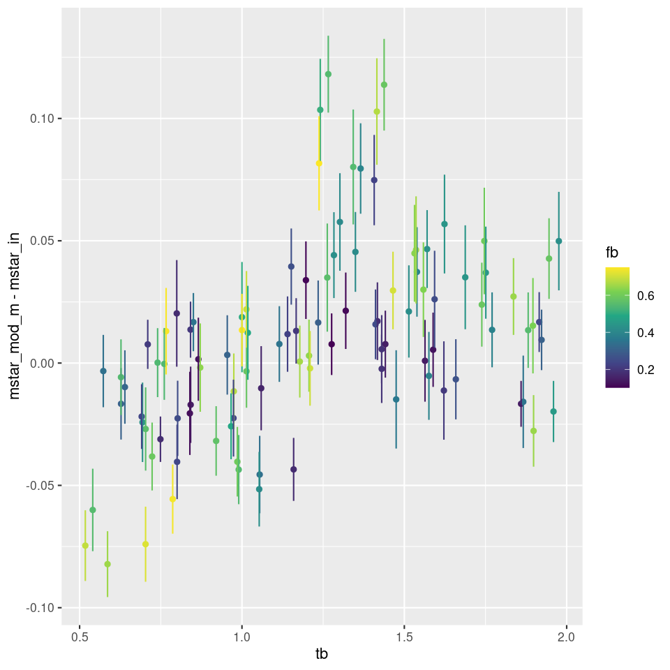
There appears to be a weak trend with burst age up to about 1 Gyr, but at all burst ages and strengths there are biases on both sides of zero. It isn’t clear to me what, if anything else, is driving biases in either direction. The one thing I can say for sure is that the models are overconfident in their ability to estimate the stellar mass since the typical 1σ error bar is under 0.02 dex while the scatter is around ±0.1 dex. I actually think 25% uncertainty in stellar mass estimates is optimistic.
I remembered a short while ago that “outshining” is the term of art in the industry for the situation in which light from recent star formation overwhelms that of the older population. This seems to be a fairly major concern in the literature. A full text search of ADS found 722 instances of its use in the astronomical literature with an explosion of usage after 2006. A quick scan of titles suggests perhaps half of the papers are about SFH modeling. Of course the word is often used in other contexts.
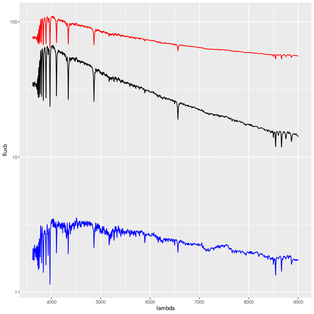
As a slightly more stringent test for outshining I ran one more simulation with a more recent and stronger starburst (tb=0.25 Gyr, fb = 1) than the earlier simulations. Even though the light of the burst population dominates the old base population the latter does have some effect of the combined spectrum (in red below, and offset vertically for clarity): it is redder and the line strengths are altered somewhat relative to the burst population.
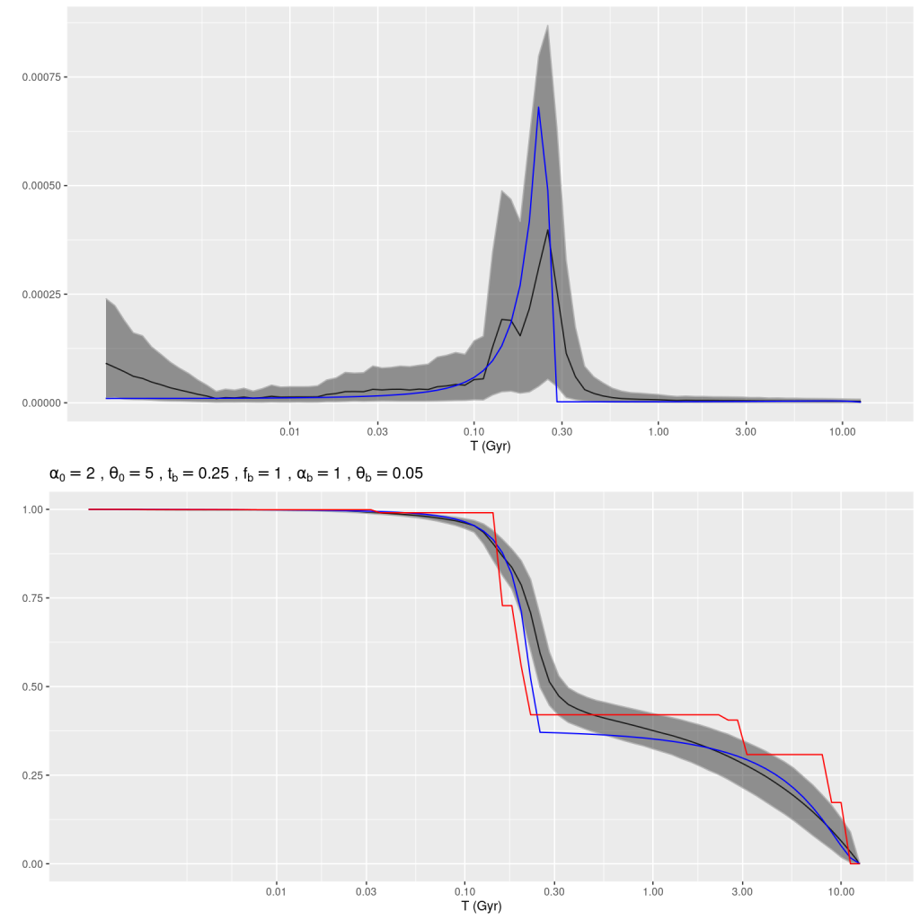
The model actually captures both the ancient and recent star formation history rather well. The mass growth marginal confidence band at old ages covers the input right up to the beginning of the burst build up, and the post-burst SFR is modeled accurately. The total mass in the model slightly exceeds the input: log(M*) = 4.88±0.02 model, 4.84 input. The model specific star formation rate is nearly identical: -9.33±0.08 model, -9.36 input.
Shortly after starting these simulations I noticed a paper by Suess et al. (2022) describing simulations with a similar objective of testing the ability of a code named PROSPECTOR to recover star formation histories of post-starburst galaxies in the ideal case of inputs matched to the model, i.e. the inputs are used to generate the mock data and then to fit it. I’m not going to say a lot about either the code or paper. IIRC the first published description of the code (Leja et al. 2017) claimed it to be the first to model non-parametric star formation histories in a fully Bayesian framework. As far as I know this is true in the published literature but they only could use a few very broad time bins; the version used in Suess uses 9. I was already using the full time resolution of my adopted SSP model libraries by then.
The 2022 paper only shows a single, no doubt cherry picked example of a fit to mock data. Like mine their model star formation histories fail to cover the inputs for some age ranges. On the other hand their fits to a mock spectrum appear to be rather poor with large systematic errors. In every model run of mine residuals look very much like 0 mean Gaussian white noise with the expected deviance. They appear to show a similar range of deviations from input stellar masses with no significant error in the mean. Another striking similarity is they find a definite floor to late time star formation rates. As I’ve noted many times my models will always include some contribution from very young populations and there seems to be a floor around 10-11.5 /yr in specific star formation rate.
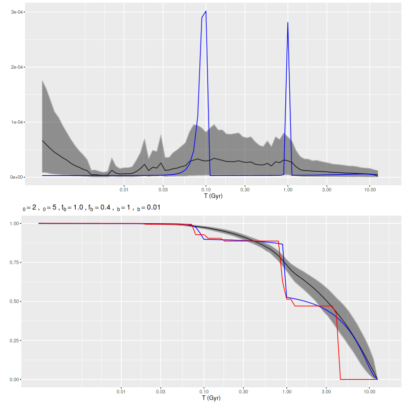
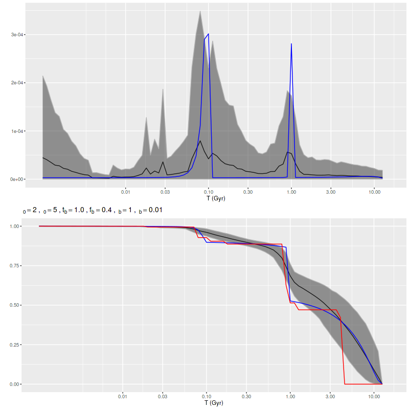
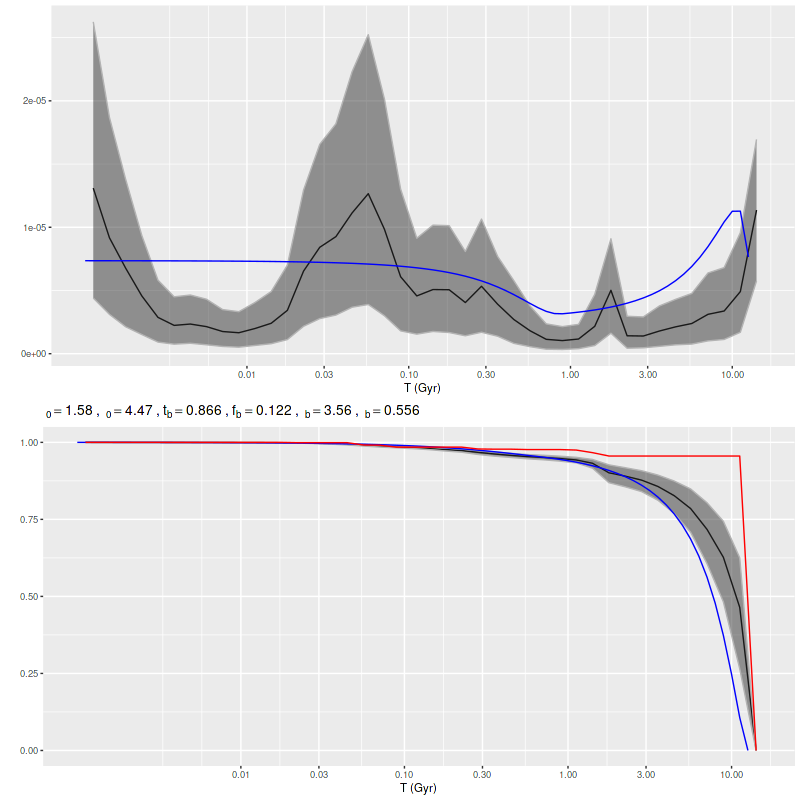
A much more recent paper by the same group (Wang et al. 2025) looked at simulated data from quite different systems, namely ones with bursty star formation on short time scales. Their work was motivated by yet more simulations of galaxy formation in the early universe. I’m again not going to comment much on this paper except to notice that they concluded that “given the correct SFH model, it is indeed possible to infer the SFH by performing SED fitting.” In other words they had to fine tune their prior to get to the right posterior. I’m sure it’s not as tautological as that sentence appears. Anyway, this motivated me to take a brief look at a few multiple burst simulations. The one shown below has two very sharply peaked ones with roughly the same peak SFR but more total mass in the older one. The model has spread out star formation over the entire interval between the input bursts with a slower rise and decay. Once again the maximum likelihood fit obtained with non-negative least squares captures the timing and relative magnitude of the bursts rather well.
Recall that my stellar contribution estimates are parametrized as an N-simplex with an implicit Dirichlet prior with concentration parameter α = 1, which is uniform on the simplex. In principle adopting an explicit prior with a concentration parameter < 1 should encourage a more bursty star formation history without favoring any particular ages, and it did (this run used α = 0.25):
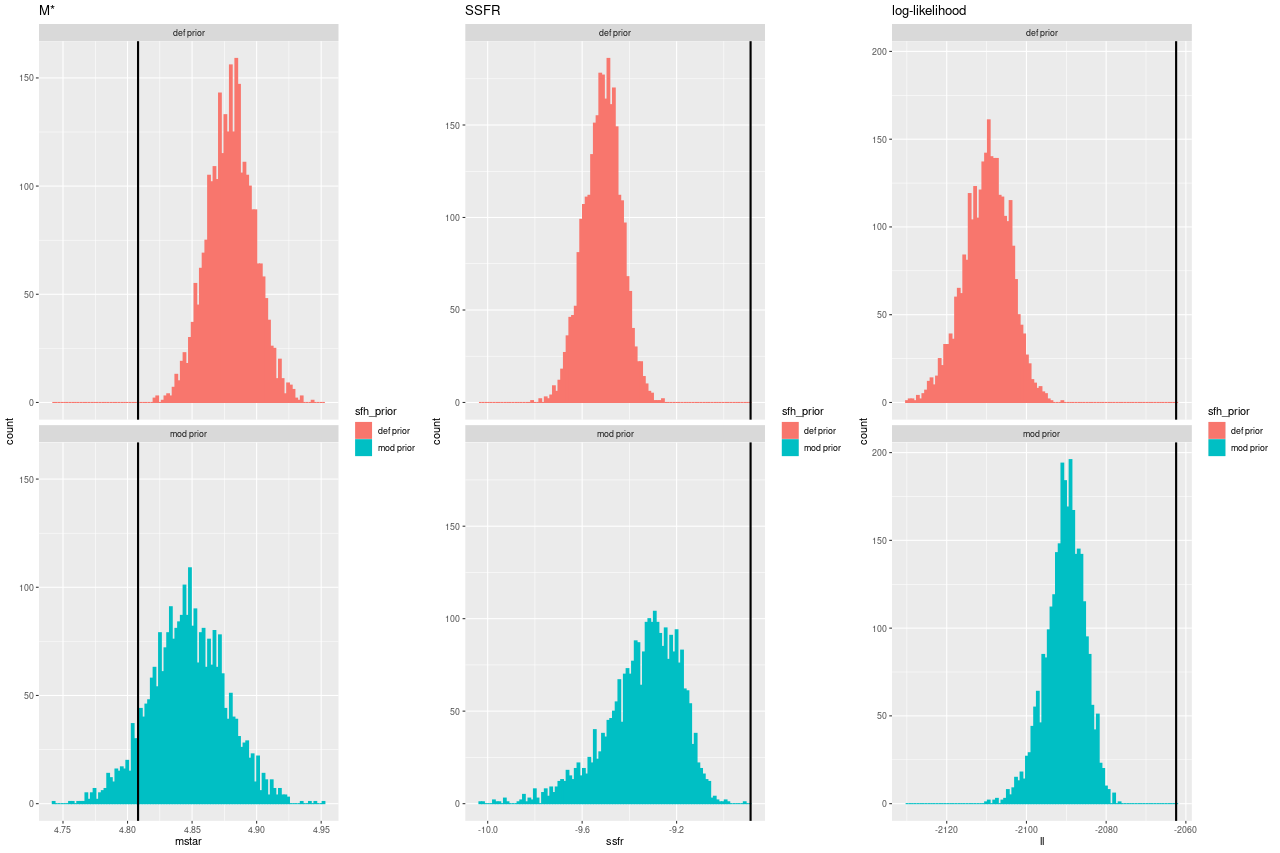
Here are histograms of a few summary quantities I track: the present day stellar mass, specific star formation rate (100 Myr average), and the summed log-likelihood of the fits to the spectra. Both runs underestimated the sSSFR because the recent burst was more spread out in the models.
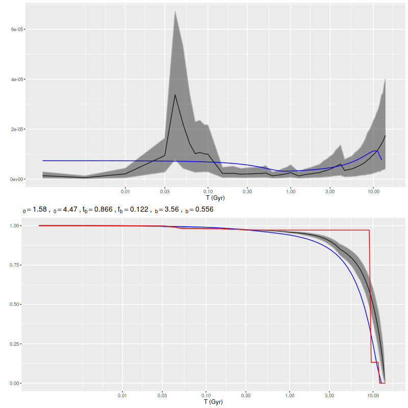
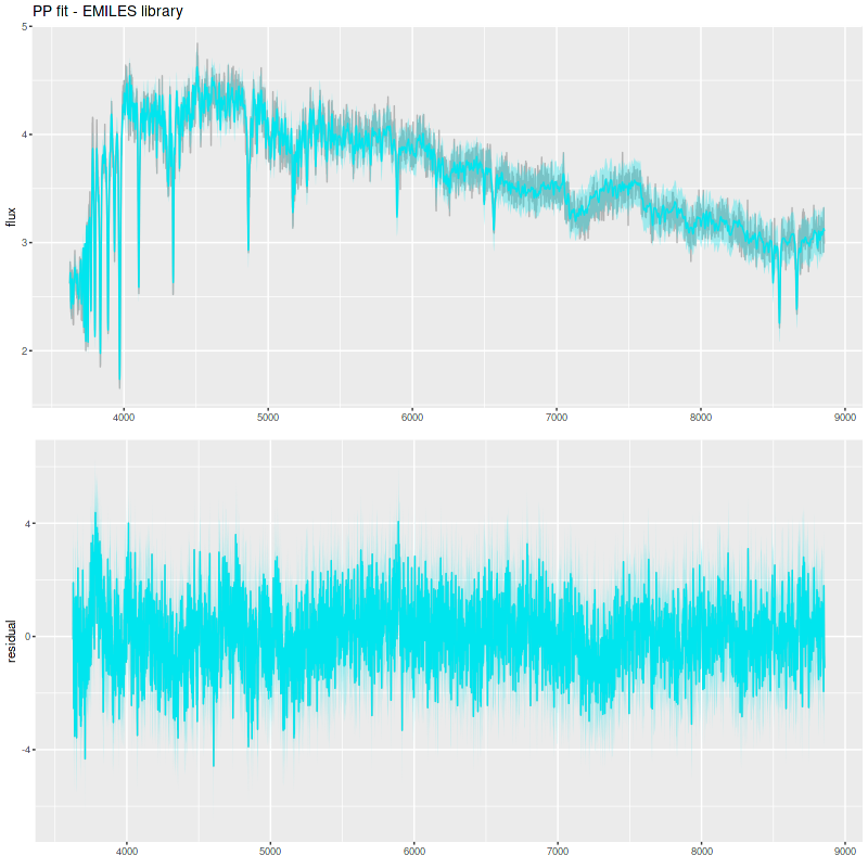
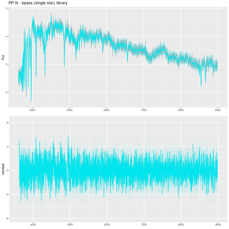
Finally, I did a few runs with two other libraries: EMILES, which has been my base SSP model library for some time, and BPASS with single star evolution and an upper mass limit of 100 M☉. The parameters I used for the star formation history resulted in a gentle late time revival rather than a burst. Both model runs had late time bursts, although the mass added was negligible. The EMILES run has the characteristic jumps at ages where the age intervals change. Although it’s small the BPASS run has the jump at 1.6 Gyr that I noted previously.
As with real data the EMILES models have some systematic errors around the trough around 7000-7300Å, and also in the blue near the Balmer break.
The BPASS models fit the data surprisingly well, despite using completely different sources for stellar atmospheres.
Comparison PP fit with C3K as test library:
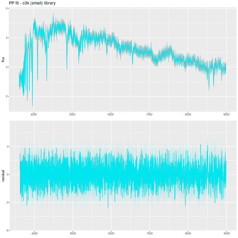
The table below summarizes a couple of the quantities I track. The Progeny C3K models that were used to create the inputs recovers them flawlessly. The other two recover the mass (BPASS is low by more than its nominal uncertainty), but are biased on the high side in late time star formation rate estimates.
| Stellar mass | sSFR | |
| input | 4.78 | -9.91 |
| Progeny C3K | 4.78 (0.017) | -9.90 (0.054) |
| EMILES | 4.82 (0.012) | -9.62 (0.028) |
| BPASS | 4.67 (0.03) | -9.73 (0.049) |
I’m going to get back to real data now using the Progeny generated libraries. The simulations were a useful exercise if for no other reason than to show that timing faded starbursts can’t be done very accurately, at least with full spectrum fitting at visual wavelengths. I did get some ideas for small code improvements, and the idea of stacking star formation rate and mass growth histories seems like a useful visualization tool.