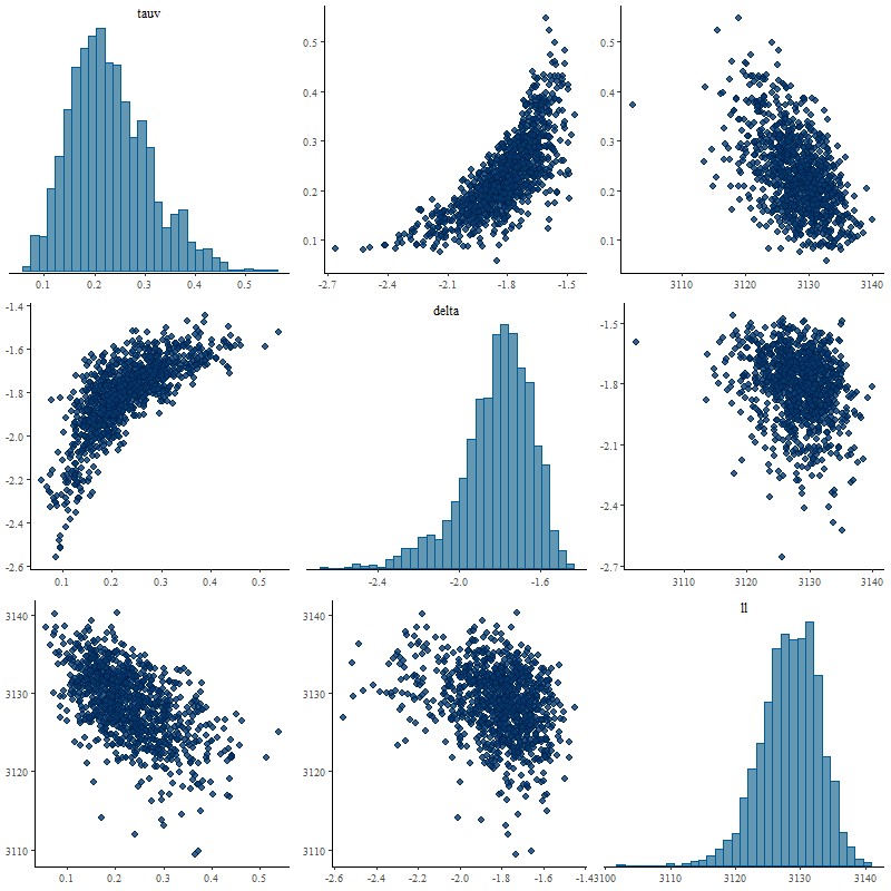
Here’s a problem that isn’t a huge surprise but that I hadn’t quite anticipated. I initially chose, without a lot of thought, a prior \(\delta \sim \mathcal{N}(0, 0.5)\) for the slope parameter delta in the modified Calzetti relation from the last post. This seemed reasonable given Salim et al.’s result showing that most galaxies have slopes \(-0.1 \lesssim \delta \lesssim +1\) (my wavelength parameterization reverses the sign of \(\delta\) ). At the end of the last post I made the obvious comment that if the modeled optical depth is near 0 the data can’t constrain the shape of the attenuation curve and in that case the best that can be hoped for is the model to return the prior for delta. Unfortunately the actual model behavior was more complicated than that for a spectrum that had a posterior mean tauv near 0:
Pairs plot of parameters tauv and delta, plus summed log likelihood with “loose” prior on delta.
Although there weren’t any indications of convergence issues in this run experts in the Stan community often warn that “banana” shaped posteriors like the joint distribution of tauv and delta above are difficult for the HMC algorithm in Stan to explore. I also suspect the distribution is multi-modal and at least one mode was missed, since the fit to the flux data as indicated by the summed log-likelihood is slightly worse than the unmodified Calzetti model.
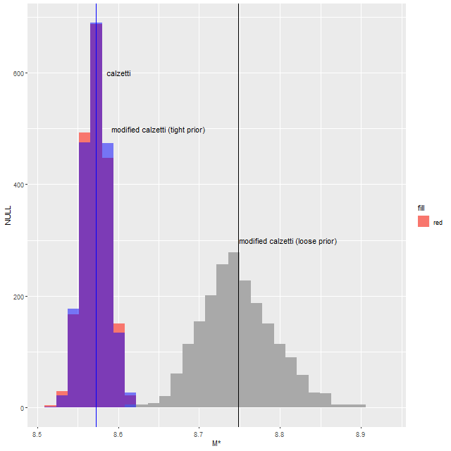
A value of \(\delta\) this small actually reverses the slope of the attenuation curve, making it larger in the red than in the blue. It also resulted in a stellar mass estimate about 0.17 dex larger than the original model, which is well outside the statistical uncertainty:
Stellar mass estimates for loose and tight priors on delta + unmodified Calzetti attenuation curve
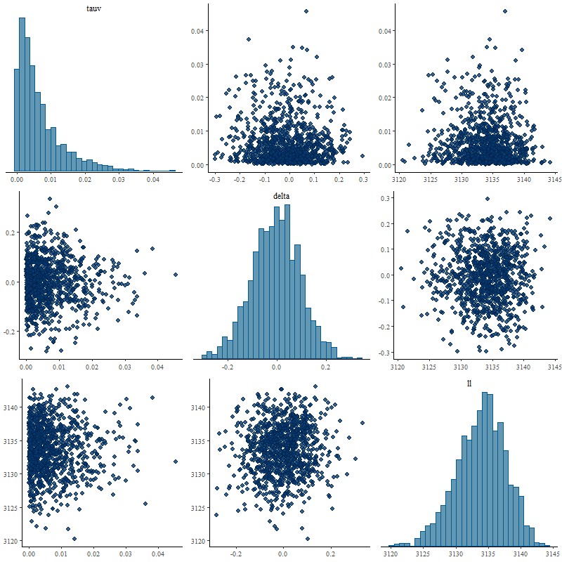
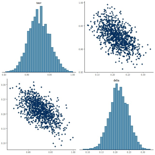
I next tried a tighter prior on delta of 0.1 for the scale parameter, with the following result:
Pairs plot of parameters tauv and delta, plus summed log likelihood with “tight” prior on delta.
Now this is what I hoped to see. The marginal posterior of delta almost exactly returns its prior, properly reflecting the inability of the data to say anything about it. The posterior of tauv looks almost identical to the original model with a very slightly longer tail:
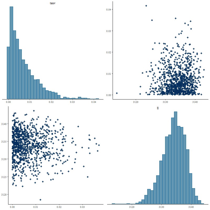
Pairs plot of parameters tauv and summed log likelihood, unmodified Calzetti attenuation curve
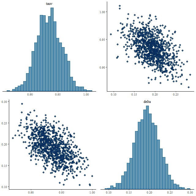
So this solves one problem but now I must worry that the prior is too tight in general since Salim’s results predict a considerably larger spread of slopes. As a first tentative test I ran another spectrum from the same spiral galaxy (this is mangaid 1-382712) that had moderately large attenuation in the original model (1.08 ± 0.04) with both “tight” and “loose” priors on delta with the following results:
Joint posterior of parameters tau and delta with “tight” priorJoint posterior of parameters tau and delta with “loose” prior
The distributions of tauv look nearly the same, while delta shrinks very slightly towards 0 with a tight prior, but with almost the same variance. Some shrinkage towards Calzetti’s original curve might be OK. Anyway, on to a larger sample.
I finally got around to reading a paper by Salim, Boquien, and Lee (2018), who proposed a simple modification to Calzetti‘s well known starburst attenuation relation that they claim accounts for most of the diversity of curves in both star forming and quiescent galaxies. For my purposes their equation 3, which summarizes the relation, can be simplified in two ways. First, for mostly historical reasons optical astronomers typically quantify the effect of dust with a color excess, usually E(B-V). If the absolute attenuation is needed, which is certainly the case in SFH modeling, the ratio of absolute to “selective” attenuation, usually written as \(\mathrm{R_V = A_V/E(B-V)}\) is needed. Parameterizing attenuation by color excess adds an unnecessary complication for my purposes. Salim et al. use a family of curves that differ only in a “slope” parameter \(\delta\) in their notation. Changing \(\delta\) changes \(\mathrm{R_V}\) according to their equation 4. But I have always parametrized dust attenuation by optical depth at V, \(\tau_V\) so that the relation between intrinsic and observed flux is
Note that parameterizing by optical depth rather than total attenuation \(\mathrm{A_V}\) is just a matter of taste since they only differ by a factor 1.08. The wavelength dependent part of the relationship is the same.
The second simplification results from the fact that the UV or 2175Å “bump” in the attenuation curve will never be redshifted into the spectral range of MaNGA data and in any case the subset of the EMILES library I currently use doesn’t extend that far into the UV. That removes the bump amplitude parameter and the second term in Salim et al.’s equation 3, reducing it to the form
The published expression for \(k(\lambda)\) in Calzetti et al. (2000) is given in two segments with a small discontinuity due to rounding at the transition wavelength of 6300Å. This produces a small unphysical discontinuity when applied to spectra, so I just made a polynomial fit to the Calzetti curve over a longer wavelength range than gets used for modeling MaNGA or SDSS data. Also, I make the wavelength parameter \(y = 5500/\lambda\) instead of using the wavelength in microns as in Calzetti. With these adjustments Calzetti’s relation is, to more digits than necessary:
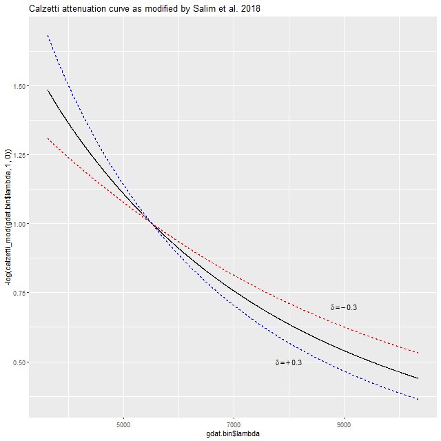
Note that δ has the opposite sign as in Salim et al. Here is what the curve looks like over the observer frame wavelength range of MaNGA. A positive value of δ produces a steeper attenuation curve than Calzetti’s, while a negative value is shallower (grayer in common astronomers’ jargon). Salim et al. found typical values to range between about -0.1 and +1.
Calzetti attenuation relation with modification proposed by Salim, Boquien, and Lee (2018). Dashed lines show shift in curve for their parameter δ = ± 0.3.
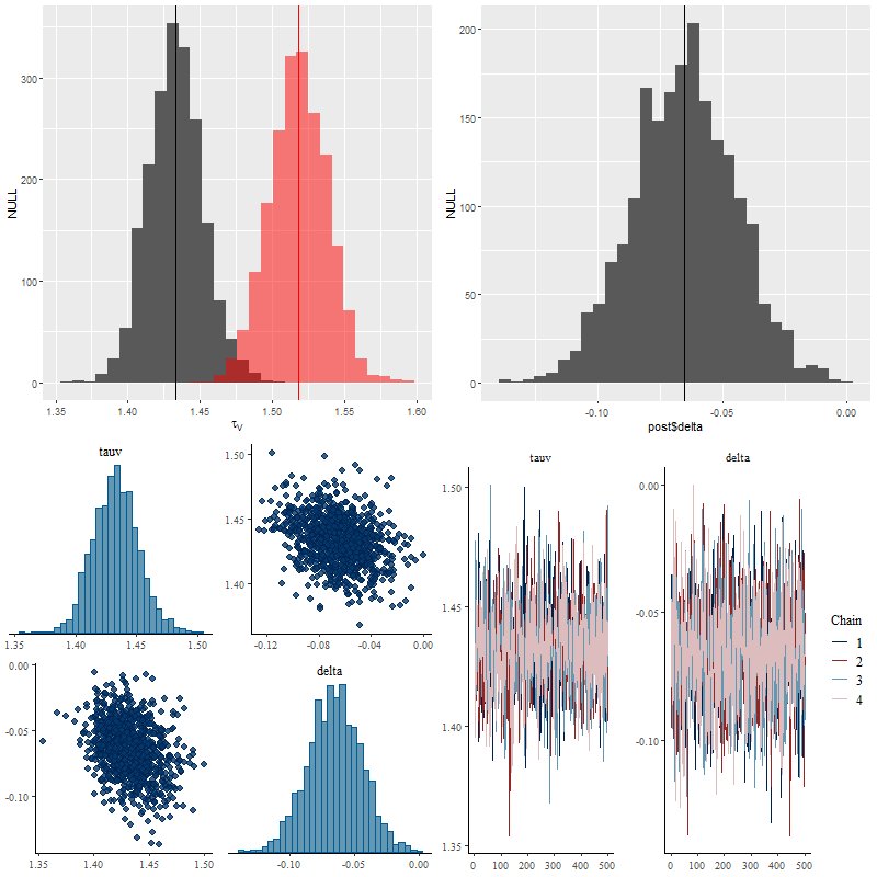
For a first pass attempt at modeling some real data I chose a spectrum from near the northern nucleus of Mrk 848 but outside the region of the highest velocity outflows. This spectrum had large optical depth \(\tau_V \approx 1.52\) and the unusual nature of the galaxy gave reason to think its extinction curve might differ significantly from Calzetti’s.
Encouragingly, the Stan model converged without difficulty and with an acceptable run time. Below are some posterior plots of the two attenuation parameters and a comparison to the optical depth parameter in the unmodified Calzetti dust model. I used a fairly informative prior of Normal(0, 0.5) for the parameter delta. The data actually constrain the value of delta, since its posterior marginal density is centered around -0.06 with a standard deviation of just 0.02. In the pairs plot below we can see there’s some correlation between the posteriors of tauv and delta, but not so much as to be concerning (yet).
(TL) marginal posteriors of optical depth parameter for Calzetti (red) and modified (dark gray) relation.
(TR) parameter δ in modified Calzetti relation
(BL) pairs plot of `tauv` and `delta`
(BR) trace plots of `tauv` and `delta`
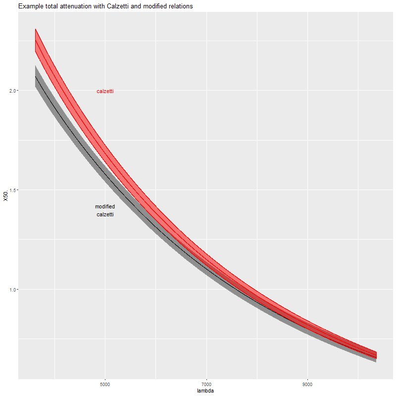
Overall the modified Calzetti model favors a slightly grayer attenuation curve with lower absolute attenuation:
Total attenuation for original and modified Calzetti relations. Spectrum was randomly selected near the northern nucleus or Mrk 848.
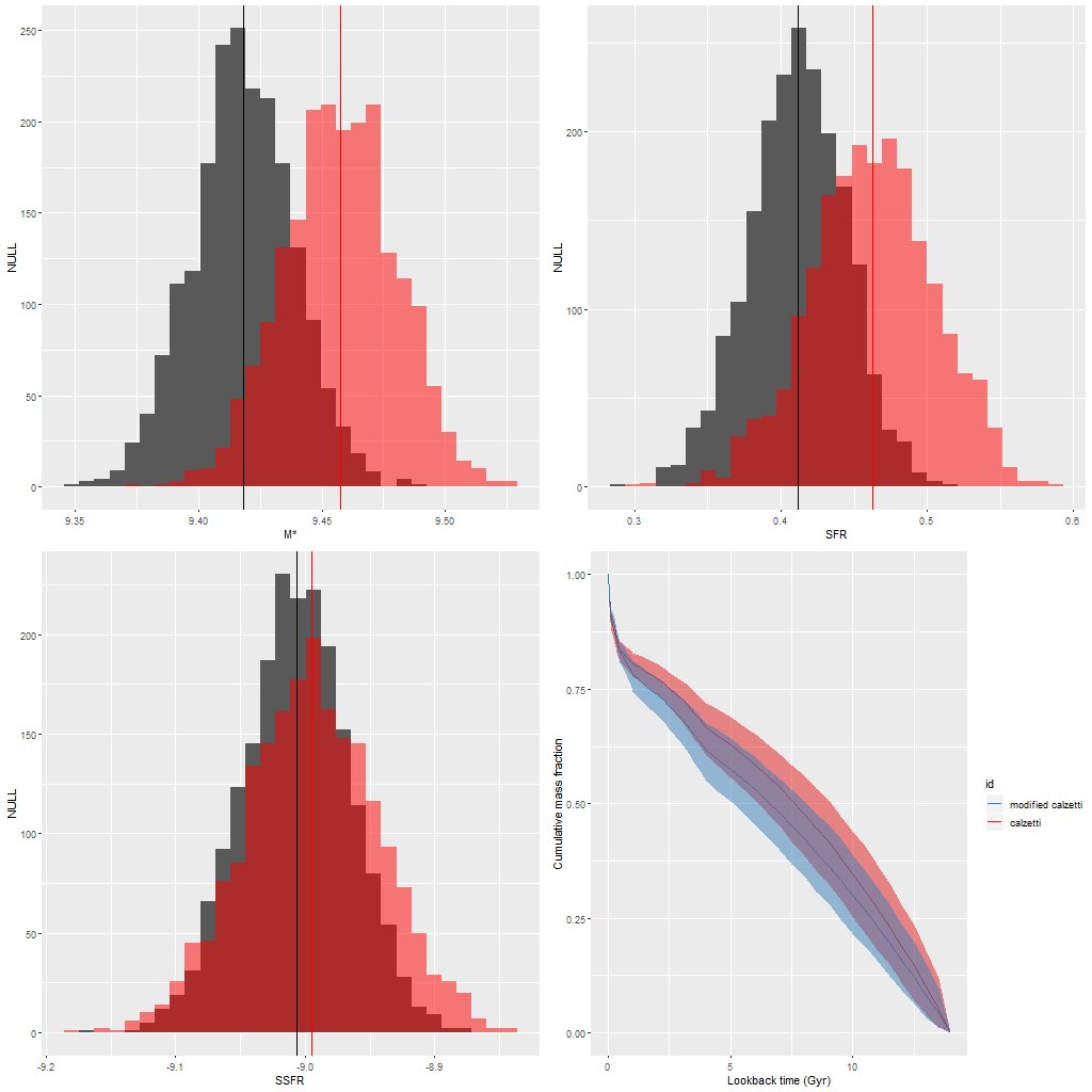
Here’s a quick look at the effect of the model modification on some key quantities. In the plot below the red symbols are for the unmodified Calzetti attenuation model, and gray or blue the modified one. These show histograms of the marginal posterior density of total stellar mass, 100Myr averaged star formation rate, and specific star formation rate. Because the modified model has lower total attenuation it needs fewer stars, so the lower stellar mass (by ≈ 0.05 dex) is a fairly predictable consequence. The star formation rate is also lower by a similar amount, making the estimates of specific star formation rate nearly identical.
The lower right pane compares model mass growth histories. I don’t have any immediate intuition about how the difference in attenuation models affects the SFH models, but notice that both show recent acceleration in star formation, which was a main theme of my Markarian 848 posts.
Stellar mass, SFR,, SSFR, and mass growth histories for original and modified Calzetti attenuation relation.
So, this first run looks ok. Of course the problem with real data is there’s no way to tell if a model modification actually brings it closer to reality — in this case it did improve the fit to the data a little bit (by about 0.2% in log likelihood) but some improvement is expected just from adding a parameter.
My concern right now is that if the dust attenuation is near 0 the data can’t constrain the value of δ. The best that can happen in this situation is for the model to return the prior. Preliminary investigation of a low attenuation spectrum (per the original model) suggests that in fact a tighter prior on delta is needed than what I originally chose.
One more post making use of the measurement error model introduced last time and then I think I move on. I estimate the dust attenuation of the starlight in my SFH models using a Calzetti attenuation relation parametrized by the optical depth at V (τV). If good estimates of Hα and Hβ emission line fluxes are obtained we can also make optical depth estimates of emission line regions. Just to quickly review the math we have:
\(A_\lambda = \mathrm{e}^{-\tau_V k(\lambda)}\)
where \(k(\lambda)\) is the attenuation curve normalized to 1 at V (5500Å) and \(A_\lambda\) is the fractional flux attenuation at wavelength λ. Assuming an intrinsic Balmer decrement of 2.86, which is more or less the canonical value for H II regions, the estimated optical depth at V from the observed fluxes is:
The SFH models return samples from the posteriors of the emission lines, from which are calculated sample values of \(\tau_V^{bd}\).
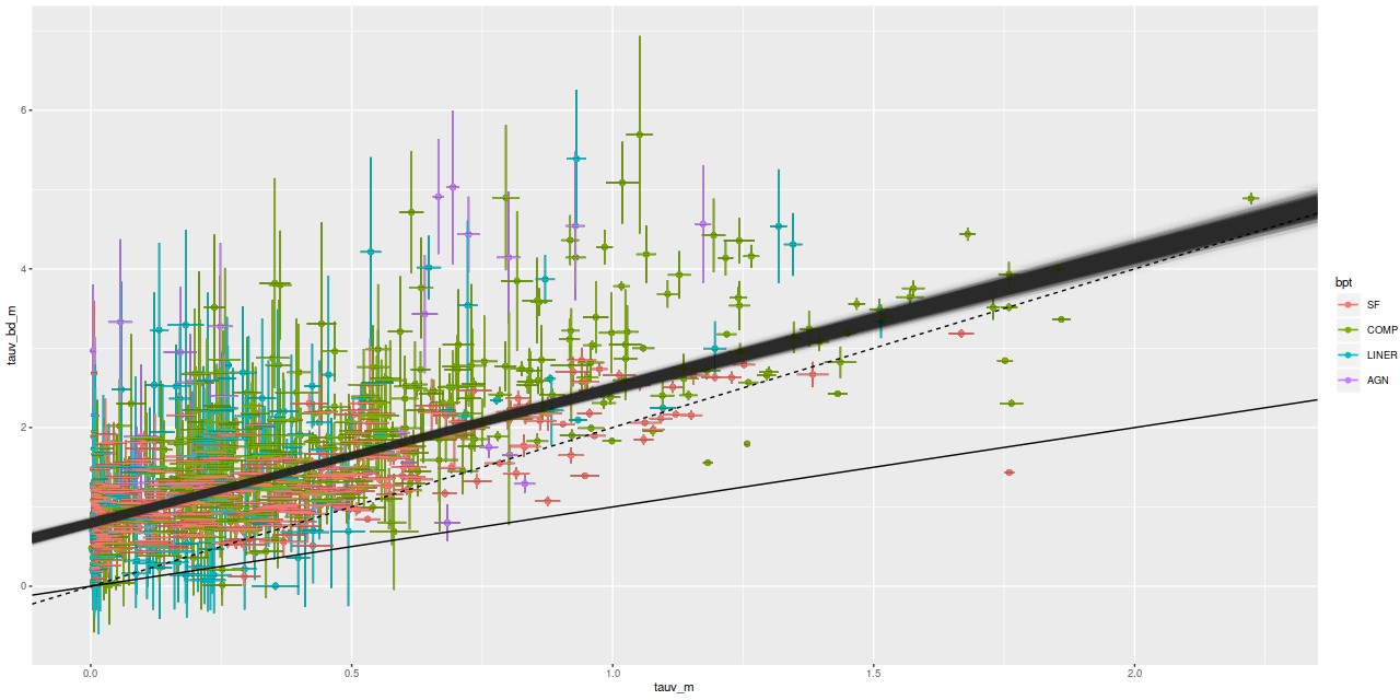
Here is a plot of the estimated attenuation from the Balmer decrement vs. the SFH model estimates for all spectra from the 28 galaxy sample in the last two posts that have BPT classifications other than no or weak emission. Error bars are ±1 standard deviation.
τVbd vs. τVstellar for 962 binned spectra in 28 MaNGA galaxies. Cloud of lines is from fit described in text. Solid and dashed lines are 1:1 and 2:1 relations.
It’s well known that attenuation in emission line regions is larger than that of the surrounding starlight, with a typical reddening ratio of ∼2 (among many references see the review by Calzetti (2001) and Charlot and Fall (2000)). One thing that’s clear in this plot that I haven’t seen explicitly mentioned in the literature is that even in the limit of no attenuation of starlight there typically is some in the emission lines. I ran the regression with measurement error model on this data set, and got the estimated relationship \(\tau_V^{bd} = 0.8 (\pm 0.05) + 1.7 ( \pm 0.09) \tau_V^{stellar}\) with a rather large estimated scatter of ≈ 0.45. So the slope is a little shallower than what’s typically assumed. The non-zero intercept seems to be a robust result, although it’s possible the models are systematically underestimating Hβ emission. I have no other reason to suspect that, though.
The large scatter shouldn’t be too much of a surprise. The shape of the attenuation curve is known to vary between and even within galaxies. Adopting a single canonical value for the Balmer decrement may be an oversimplification too, especially for regions ionized by mechanisms other than hot young stars. My models may be overdue for a more flexible prescription for attenuation.
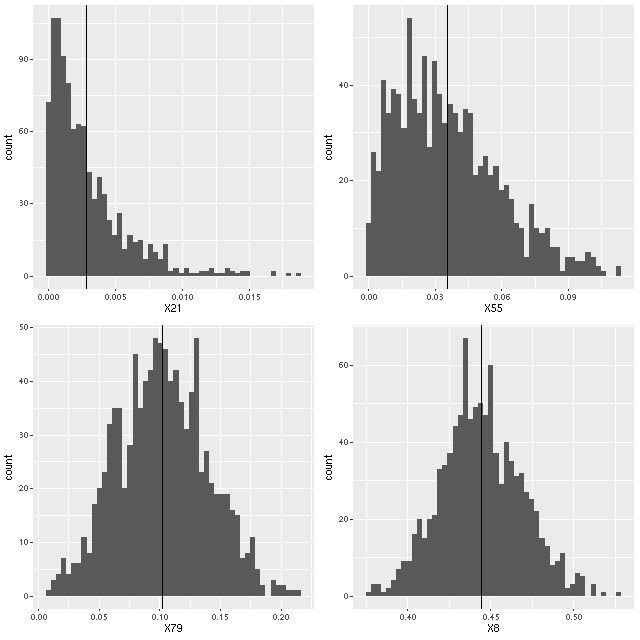
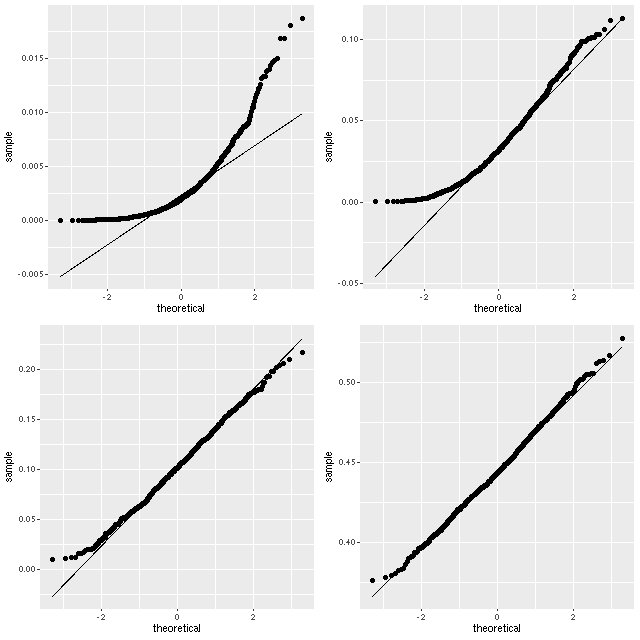
The statistical assumptions of the measurement error model are a little suspect in this data set as well. The attenuation parameter tauv is constrained to be positive in the models. When it wants to be near 0 the samples from the posterior will pile up near 0 with a tail of larger values, looking more like draws from an exponential or gamma distribution than a gaussian. Here is an example from one galaxy in the sample that happens to have a wide range of mean attenuation estimates:
Histograms of samples from the marginal posterior distributions of the parameter tauv for 4 spectra from plateifu 8080-3702.
I like theoretical quantile-quantile plots better than histograms for this type of visualization:
Normal quantile-quantile plots of samples from the marginal posterior distributions of the parameter tauv for 4 spectra from plateifu 8080-3702.
I haven’t looked at the distributions of emission line ratios in much detail. They might behave strangely in some cases too. But regardless of the validity of the statistical model applied to this data set it’s apparent that there is a fairly strong correlation, which is encouraging.
Here’s a pretty common situation with astronomical data: two or more quantities are measured with nominally known uncertainties that in general will differ between observations. We’d like to explore the relationship among them, if any. After graphing the data and establishing that there is a relationship a first cut quantitative analysis would usually be a linear regression model fit to the data. But the ordinary least squares fit is biased and might be severely misleading if the measurement errors are large enough. I’m going to present a simple measurement error model formulation that’s amenable to Bayesian analysis and that I’ve implemented in Stan. This model is not my invention by the way — in the astronomical literature it dates at least to Kelly (2007), who also explored a number of generalizations. I’m only going to discuss the simplest case of a single predictor or covariate, and I’m also going to assume all conditional distributions are gaussian.
The basic idea of the model is that the real, unknown quantities (statisticians call these latent variables, and so will I) are related through a linear regression. The conditional distribution of the latent dependent variable is
where \(\sigma_{x, i}, \sigma_{y, i}\) are the known standard deviations. The full joint distribution is completed by specifying priors for the parameters \(\beta_0, \beta_1, \sigma\). This model is very easy to implement in the Stan language and the complete code is listed below. I’ve also uploaded the code, a script to reproduce the simulated data example discussed below, and the SFR-stellar mass data from the last page in a dropbox folder.
Most of this code should be self explanatory, but there are a few things to note. In the transformed data section I standardize both variables, that is I subtract the means and divide by the standard deviations. The individual observation standard deviations are also scaled. The transformed parameters block is strictly optional in this model. All it does is spell out the linear part of the linear regression model.
In the model block I give a very vague prior for the latent x variables. This has almost no effect on the model output since the posterior distributions of the latent values are strongly constrained by the observed data. The parameters of the regression model are given less vague priors. Since we standardized the data we know beta0 should be centered near 0 and beta1 near 1 and all three should be approximately unit scaled. The rest of the model block just encodes the conditional distributions I wrote out above.
Finally the generated quantities block does two things: generate some some new simulated data values under the model using the sampled parameters, and rescale the parameter values to the original data scale. The first task enables what’s called “posterior predictive checking.” Informally the idea is that if the model is successful simulated data generated under it should look like the data that was input.
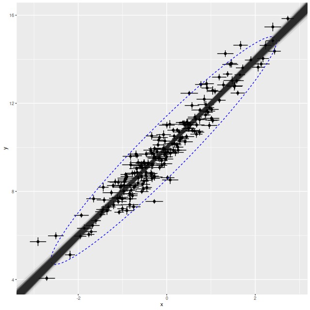
It’s always a good idea to try out a model with some simulated data that conforms to it, so here’s a script to generate some data, then print and graph some basic results. This is also in the dropbox folder.
Inference for Stan model: ls_me.
4 chains, each with iter=2000; warmup=1000; thin=1;
post-warmup draws per chain=1000, total post-warmup draws=4000.

             mean se_mean    sd  2.5%   25%   50%    75%  97.5% n_eff  Rhat
b0          9.995   0.001 0.042 9.912 9.966 9.994 10.023 10.078  5041 0.999
b1          1.993   0.001 0.040 1.916 1.965 1.993  2.020  2.073  4478 1.000
sigma_unorm 0.472   0.001 0.037 0.402 0.447 0.471  0.496  0.549  2459 1.003

Samples were drawn using NUTS(diag_e) at Thu Jan  9 10:09:34 2020.
For each parameter, n_eff is a crude measure of effective sample size,
and Rhat is the potential scale reduction factor on split chains (at
convergence, Rhat=1).
>
and graph:
Simulated data and model fit from script in text. Ellipse is 95% confidence interval for new data generated from model.
This all looks pretty good. The true parameters are well within the 95% confidence bounds of the estimates. In the graph the simulated new data is summarized with a 95% confidence ellipse, which encloses just about 95% of the input data, so the posterior predictive check indicates a good model. Stan is quite aggressive at flagging potential convergence failures, and no warnings were generated.
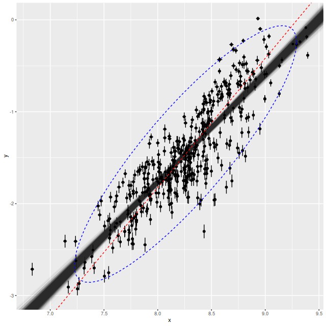
Turning to some real data I also included in the dropbox folder the star formation rate density versus stellar mass density data that I discussed in the last post. This is in something called R “dump” format, which is just an ascii file with R assignment statements for the input data. This isn’t actually a convenient form for input to rstan’s sampler or ggplot2’s plotting commands, so once loaded the data are copied into a list and a data frame. The interactive session for analyzing the data was:
Star formation rate vs. Stellar mass for star forming regions. Data from previous post.
Semi-transparent lines – model fits to the regression line as described in text.
Dashed red line – “orthogonal distance regression” fit.
Inference for Stan model: ls_me.
4 chains, each with iter=2000; warmup=1000; thin=1;
post-warmup draws per chain=1000, total post-warmup draws=4000.

              mean se_mean   sd   2.5%    25%    50%    75%  97.5% n_eff Rhat
b0          -11.20       0 0.26 -11.73 -11.37 -11.19 -11.02 -10.67  7429    1
b1            1.18       0 0.03   1.12   1.16   1.18   1.20   1.24  7453    1
sigma_unorm   0.27       0 0.01   0.25   0.27   0.27   0.28   0.29  7385    1

Samples were drawn using NUTS(diag_e) at Thu Jan  9 10:49:42 2020.
For each parameter, n_eff is a crude measure of effective sample size,
and Rhat is the potential scale reduction factor on split chains (at
convergence, Rhat=1).
Once again the model seems to fit the data pretty well, the posterior predictive check is reasonable, and Stan didn’t complain. Astronomers are often interested in the “cosmic variance” of various quantities, that is the true amount of unaccounted for variation. If the error estimates in this data set are reasonable the cosmic variance in SFR density is estimated by the parameter σ. The mean estimate of around 0.3 dex is consistent with other estimates in the literature1see the compilation in the paper by Speagle et al. that I cited last time, for example.
I noticed in preparing the last post that several authors have used something called “orthogonal distance regression” (ODR) to estimate the star forming main sequence relationship. I don’t know much about the technique besides that it’s an errors in variables regression method. There is an R implementation in the package pracma. The red dashed line in the plot above is the estimate for this dataset. The estimated slope (1.41) is much steeper than the range of estimates from this model. On casual visual inspection though it’s not clearly worse at capturing the mean relationship.
It took a few months but I did manage to analyze 28 of the 29 galaxies in the sample I introduced last time. One member — mangaid 1-604907 — hosts a broad line AGN and has broad emission lines throughout. That’s not favorable for my modeling methods, so I left it out. It took a while to develop a more or less standardized analysis protocol, so there may be some variation in S/N cuts in binning the spectra and in details of model runs in Stan. Most runs used 250 warmup and 750 total iterations for each of 4 chains run in parallel, with some adaptation parameters changed from their default values1I set target acceptance probability adapt_delta to 0.925 or 0.95 and the maximum treedepth for the No U-Turn Sampler max_treedepth to 11-12. A total post-warmup sample size of 2000 is enough for the inferences I want to make. One of the major advantages of the NUTS sampler is that once it converges it tends to produce draws from the posterior with very low autocorrelation, so effective sample sizes tend to be close to the number of samples.
I’m just going to look at a few measured properties of the sample in this post. In future ones I may look in more detail at some individual galaxies or the sample as a whole. Without a control sample it’s hard to say if this one is significantly different from a randomly chosen sample of galaxies, and I’m not going to try. In the plots shown below each point represents measurements on a single binned spectrum. The number of binned spectra per galaxy ranged from 15 to 153 with a median of 51.5, so a relatively small number of galaxies contribute disproportionately to these plots.
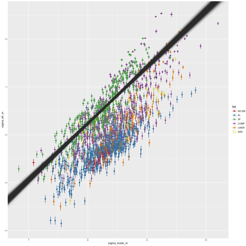
One of the more important empirical results in extragalactic astrophysics is the existence of a fairly well defined and approximately linear relationship between stellar mass and star formation rate for star forming galaxies, which has come to be known as the “star forming main sequence.” Thanks to CALIFA and MaNGA it’s been established in recent years that the SFMS extends to subgalactic scales as well, at least down to the ∼kpc resolution of these surveys. This first plot is of the star formation rate surface density vs. stellar mass surface density, where recall my estimate of SFR is for a time scale of 100 Myr. Units are \(\mathrm{M_\odot /yr/kpc^2} \) and \(\mathrm{M_\odot /kpc^2} \), logarithmically scaled. These estimates are uncorrected for inclination and are color coded by BPT class using Kauffmann’s classification scheme for [N II] 6584, with two additional classes for spectra with weak or no emission lines.
If we take spectra with star forming line ratios as comprising the SFMS there is a fairly tight relation: the cloud of lines are estimates from a Bayesian simple linear regression with measurement error model fit to the points with star forming BPT classification only (N = 428). The modeled relationship is \(\Sigma_{sfr} = -11.2 (\pm 0.5) + 1.18 (\pm 0.06)~ \Sigma_{M^*}\) (95% marginal confidence limits), with a scatter around the mean relation of ≈ 0.27 dex. The slope here is rather steeper than most estimates2For example in a large compilation by Speagle et al. (2014) none of the estimates exceeded a slope of 1., but perhaps coincidentally is very close to an estimate for a small sample of MaNGA starforming galaxies in Lin et al. (2019). I don’t assign any particular significance to this result. The slope of the SFMS is highly sensitive to the fitting method used, the SFR and stellar mass calibrators, and selection effects. Also, the slope and intercept estimates are highly correlated for both Bayesian and frequentist fitting methods.
One notable feature of this plot is the rather clear stratification by BPT class, with regions having AGN/LINER line ratios and weak emission line regions offset downwards by ~1 dex. Interestingly, regions with “composite” line ratios straddle both sides of the main sequence, with some of the largest outliers on the high side. This is mostly due to the presence of Markarian 848 in the sample, which we saw in recent posts has composite line ratios in most of the area of the IFU footprint and high star formation rates near the northern nucleus (with even more hidden by dust).
Σsfr vs. ΣM*. Cloud of straight lines is an estimate of the star-forming main sequence relation based on spectra with star-forming line ratios. Sample is all analyzed spectra from the set of “transitional” candidates of the previous post.
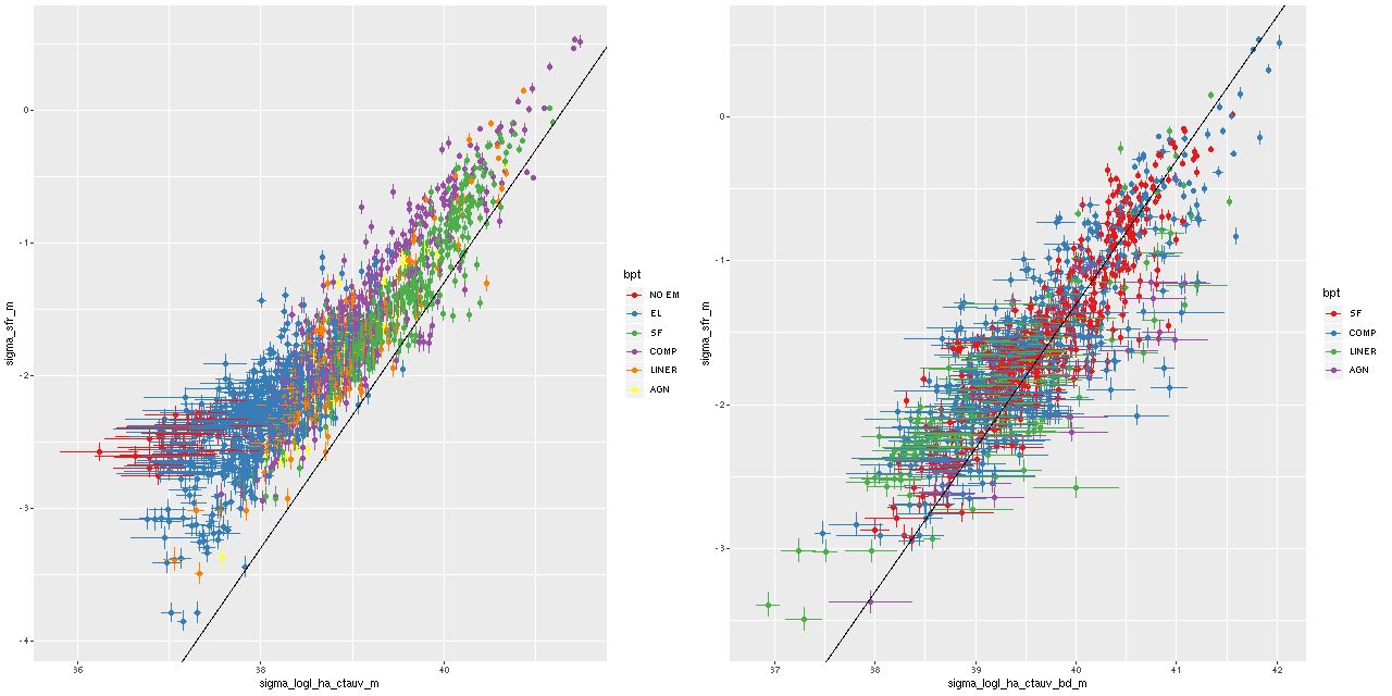
Another notable relationship that I’ve shown previously for a few individual galaxies is between the star formation rate estimated from the SFH models and Hα luminosity, which is the main SFR calibrator in optical spectra. In the left hand plot below Hα is corrected for the estimated attenuation for the stellar component in the SFH models. The straight line is the SFR-Hα calibration of Moustakas et al. (2006), which can be traced back to early ’90s work by Kennicutt.
Most of the sample does follow a linear relationship between SFR density and Hα luminosity density with an offset from the Kennicutt-Moustakas calibration, but there appears to be a departure from linearity at the low SFR end in the sense that the 100 Myr averaged SFR exceeds the amount predicted by Hα (which recall traces star formation on 5-10 Myr scales). This might be interpreted as indicating that the sample includes a significant number of regions that have been very recently quenched (that is within the past 10-100 Myr). There are other possible interpretation though, including biased estimates of Hα luminosity when emission lines are weak.
In the right hand panel below I plot the same relationship but with Hα corrected for attenuation using the Balmer decrement for spectra with firm detections in the four lines that go into the [N II]/Hα vs. [O III]/Hβ BPT classification, and therefore have firm detections in Hβ. The sample now nicely straddles the calibration line over the ∼ 4 orders of magnitude of SFR density estimates. So, the attenuation in the regions where emission lines arise is systematically higher than the estimated attenuation of stellar light. This is a well known result. What’s encouraging is it implies my model attenuation estimates actually contain useful information.
(L) Estimated Σsfr vs. Σlog L(Hα) corrected for attenuation using stellar attenuation estimate.
(R) same but Hα luminosity corrected using Balmer decrement. Spectra with detected Hβ emission only.
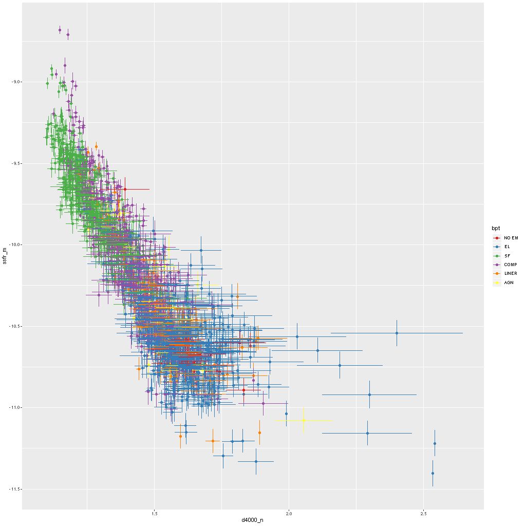
One final relation: some measure of the 4000Å break strength has been used as a calibrator of specific star formation rate since at least Brinchmann et al. (2004). Below is my version using the “narrow” definition of D4000. I haven’t attempted a quantitative comparison with any other work, but clearly there’s a well defined relationship. Maybe worth noting is that “red and dead” ETGs typically have \(\mathrm{D_n(4000)} \gtrsim 1.75\) (see my previous post for example). Very few of the spectra in this sample fall in that region, and most are low S/N spectra in the outskirts of a few of the galaxies.
Specific star formation rate vs. Dn4000
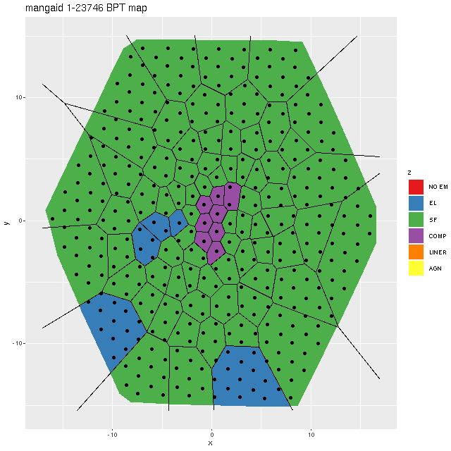
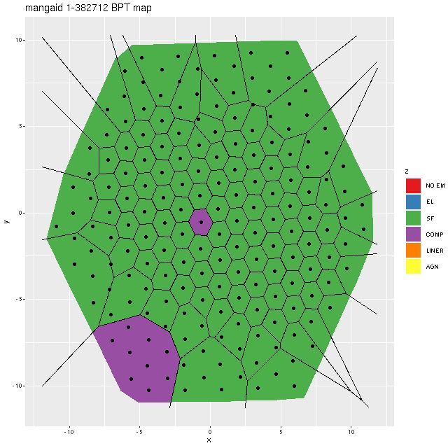
Two obvious false positives in this sample were a pair of grand design spirals (mangaids 1-23746 and 1.382712) with H II regions sprinkled along the full length of their arms. To see why they were selected and verify that they’re in fact false positives here are BPT maps:
Map of BPT classification — mangaid 1-23746 (plateifu 8611-12702)Map of BPT classification — mangaid 1-382712 (plateifu 9491-6101)
These are perfect illustrations of the perils of using single fiber spectra for sample selection when global galaxy properties are of interest. The central regions of both galaxies have “composite” spectra, which might actually indicate that the emission is from a combination of AGN and star forming regions, but outside the nuclear regions star forming line ratios prevail throughout.
These two galaxies contribute about 45% of the binned spectra with star forming line ratios, so the SFMS would be much more sparsely populated without their contribution. Only one other galaxy (mangaid 1-523050) is similarly dominated by SF regions and it has significantly disturbed morphology.
I may return to this sample or individual members in the future. Probably my next posts will be about Bayesian modelling though.