It took longer than I had hoped, but I finally have the R and Stan software that I use for star formation history modeling under version control and uploaded to github. There are 3 R packages, two of which are newly available:
spmutils: The actual code for maximum likelihood and Bayesian modeling of star formation histories. There are also tools for reading FITS files from SDSS single fiber spectra and from MaNGA, visualization, and analysis.
cosmo: A simple, lightweight cosmological distance calculator.
sfdmap: A medium resolution version of the all sky dust map of Schlegel, Finkbeiner and Davis (SFD) and a pair of functions for rapid access.
So far only cosmo is documented to minimal R standards. It’s also the most generally useful, at least if you need to calculate cosmological distances. sfdmap has skeleton help files; spmutils not even that. I plan to correct that, but probably not in the next several weeks.
The R packages are pure R code and can be installed directly from github using devtools:
The Stan files for SFH modeling that I’m currently working with are in spmutils/stan. I keep the Stan files in the directory ~/spmcode on my local machines, and that’s the default location in the functions that call them.
This code mushroomed over a period of several years without much in the way of design, so it’s not much use without some documentation of typical workflow. I will get around to that sometime soon (I hope).
In the last post I showed that the posterior distribution of the model parameters as estimated by Stan look rather different than the distribution of maximum likelihood estimates under repeated realizations of the noisy “observation” vector, but I didn’t really discuss why they look different. For starters it’s not because the Stan model failed to converge, nor is there any evidence for missed multimodality in the posterior. Although Stan threw some warnings for this model run they involved fewer than 1% of the post-warmup iterations and there was no sign of pathological behavior (by the way I recommend the package shinystan for a holistic look at Stan model outputs). Multimodality can happen — often it manifests as one or more chains converging to different distributions than the others, but sometimes Stan can fail to find extra modes. But I haven’t seen any evidence for this in repeated runs of this and similar models, nor for that matter in real data SFH modeling.I mentioned that I copied the prior over from my real data models and this is probably not quite what I wanted to use, and that gets us into the topic of investigating the effect of the prior in shaping the posterior. That’s not what caused the difference either, but I’ll look at it anyway.
The real reason I think is one that I still find paradoxical or at least sorta counterintuitive. The main task of computational Bayesian inference is to explore the “typical set” (a concept borrowed from information theory). There’s a nice case study by one of Stan’s principal developers showing through geometric arguments and some simple simulations that the typical set can be, and usually is, far (in the sense of Euclidean distance) from the most likely value and the distance increases with increasing dimensionality of the parameter space. We can show directly that is happening here.
Let’s first modify the model to adopt an improper uniform prior on the positive orthant, which just requires removing a line from the model block of the Stan code (if no prior is specified it is implicitly made uniform, which in this case is improper):
parameters {
  vector<lower=0.>[M] beta;
}
model {
  y ~ normal(X * beta, sdev);
}
Modern Bayesians usually recommend against the use of improper priors, but since the likelihood in this model is Gaussian the posterior is proper. The virtue of this model is the maximum a posteriori (MAP) solution is also the maximum likelihood solution. Stan can do general nonlinear optimization as well as sampling, using by the way conventional gradient based algorithms rather than Monte Carlo optimization.
First, I run the sampler on this model, and extract the posterior:
I do this to get a starting guess for the optimizer and because we’ll do some comparisons later. For some reason rstan’s optimization function requires as input a stanmodel object rather than a file name, so we call stan_model() to get one. Then I call the optimizer, adjusting a few parameters to try to get to a better solution than with defaults:
Now let’s use these to initialize the chains for another Stan model run (I also adjusted some of the control parameters to get rid of warnings from the first run):
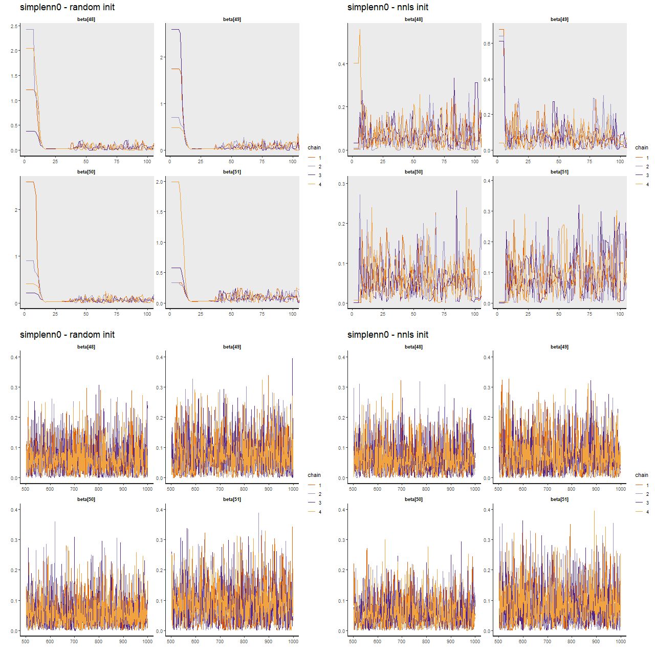
Now examine trace plots for the first few warmup draws for a few parameters. The top rows trace the first 100 warmup iterations. The right 4 are initialized with the approximate maximum likelihood solution, the left are from the first randomly initialized run. The ML initialized chains quickly move away from that point and reach stationary, well mixed distributions in just a few iterations. The randomly initialized chains take slightly longer to get to the same stationary distributions.
Stan runs with improper uniform prior – sample traceplots (TL) warmup iterations with random inits (TR) warmup iterations with nnls solution inits (BL) post-warmup with random inits (BR) post-warmup with nnls solution inits
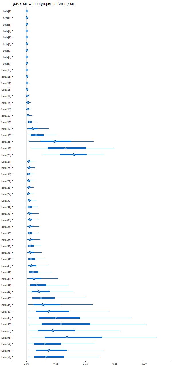
And the resulting interval plot for the model coefficients isn’t noticeably different from the first run:
Coefficient posteriors with improper uniform prior
Nowadays Bayesians generally advise using proper priors that reflect available domain knowledge. I had done that originally but without thinking that the prior wasn’t quite right given the data manipulations that I had performed. A better prior that incorporates “domain” knowledge without being too specific might be something like a truncated normal with the same scale parameter for each coefficient, which in this case can reasonably be set to 1. That’s accomplished by adding back just one line to the model block:
model {
  beta ~ normal(0, 1.);
  y ~ normal(X * beta, sdev);
}
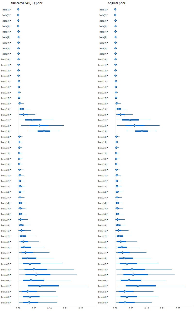
which leads to the following posterior interval plot compared to the original:
(L) N(0, 1) prior (R) original variable width prior
See the difference? Close inspection will show some minor ones, but it’s not immediately clear if they’re larger than expected from sampling variations.
Can we induce sparsity?
Here are a couple ideas I thought might work but didn’t. One way to induce sparsity in regression models is called the lasso, or more technically L-1 penalized regression. This is just least squares with an added penalty proportional to the absolute values of the model parameters. A more or less equivalent idea in Bayesian statistics is to add a double exponential or Laplacian prior. Since the parameters here are non-negative we can use an exponential prior instead.
Yet another possible prior inspired by “domain knowledge” is to notice that the coefficient values I picked sum to 1. A sum to 1 constraint can be programmed in Stan by declaring the parameter vector to be a simplex. Leaving out an explicit prior will give the parameters implicitly uniform priors.
parameters {
  simplex[M] beta;
}
model {
  y ~ normal(X * beta, sdev);
}
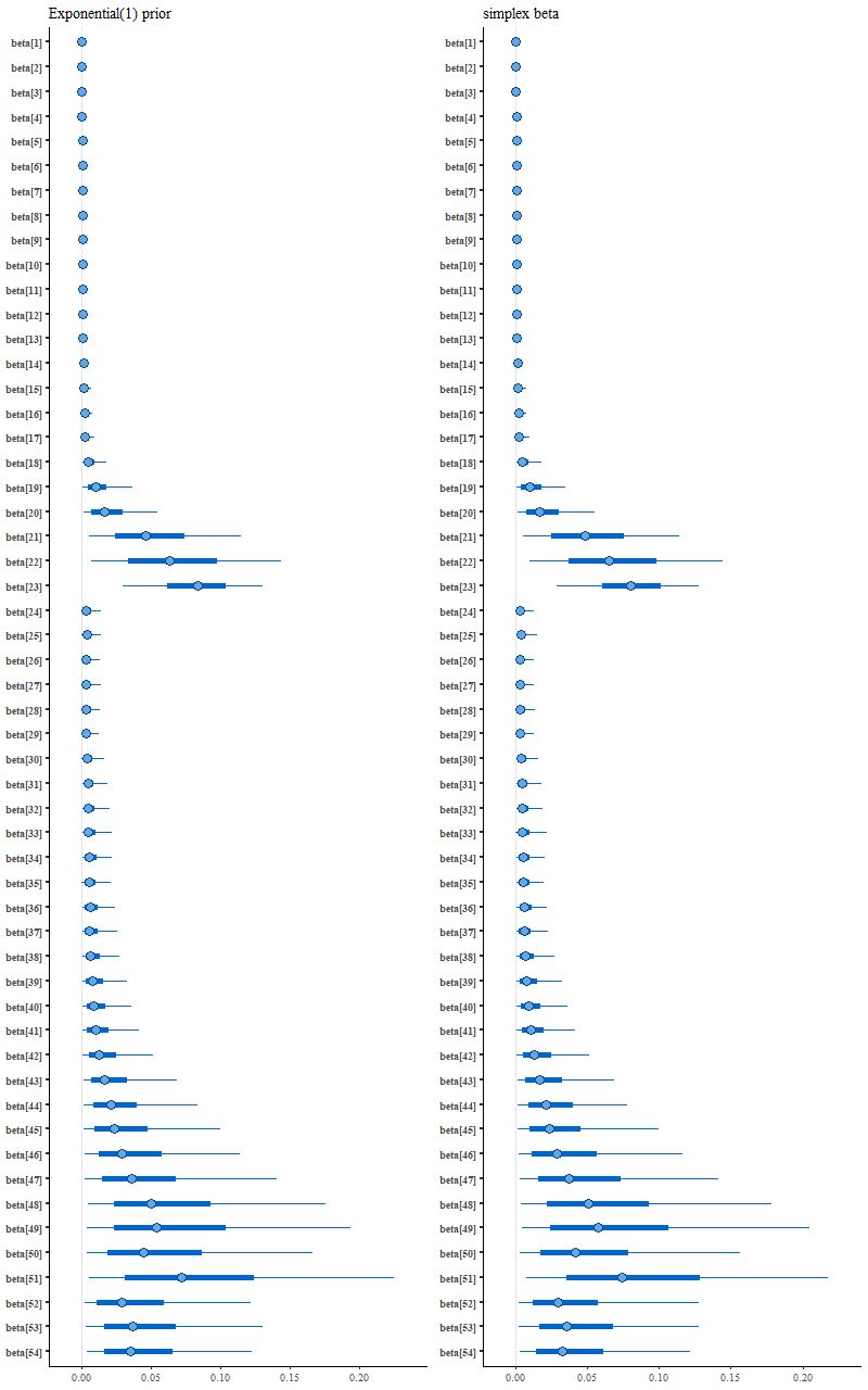
Interestingly enough for possible future reference this model ran much faster than the others and threw no warnings, but it didn’t produce a sparse solution:
More posterior interval plots (L) exponential prior (R) unit simplex parameter vector
Back to the drawing board and with a bit of web research it turns out there is a fairly standard sparsity inducing prior known as the “horseshoe” described in yet another Stan case study by another principal developer, Michael Betancourt. The parameter and model block for this looks like
parameters {
  vector<lower=0.>[M] beta;
  real<lower=0.> tau;
  vector<lower=0.>[M] lambda;
}
model {
  tau ~ cauchy(0, 0.05);
  lambda ~ cauchy(0, 1.);
  beta ~ normal(0, tau*lambda);
  y ~ normal(X * beta, sdev);
}
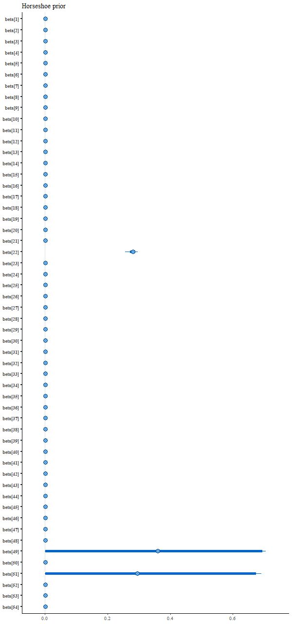
This is the “classical” horseshoe rather than the preferred prior that Betancourt refers to as the “Finnish horseshoe.” This took some fiddling with hyperparameter values to produce something sensible that appeared to converge, but it did indeed produce a sparse posterior:
Posterior intervals – Horseshoe prior
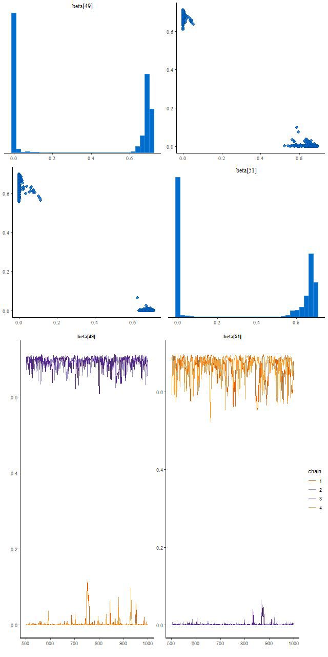
This run did find two posterior modes, and this illustrates the typical Stan behavior I mentioned at the beginning of this post. Two chains found a mode where beta[49] is large and beta[51] near 0, and two found one with the values reversed. There’s no jumping between modes within a chain:
A bimodal posterior
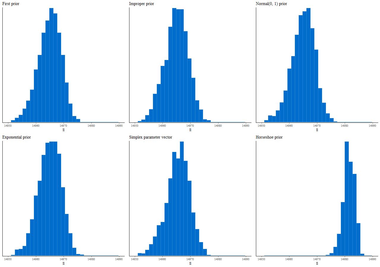
Finally, here are the distributions of log-likelihood for the 6 priors considered in the last two posts:
Posterior distributions of log-likelihood for 6 priors
Should we care about sparsity? In statistics and machine learning sparsity is usually considered a virtue because one often has a great many potential predictors, only a few of which are thought to have any real predictive value. In star formation history modeling on the other hand astronomers usually think of star formation as varying relatively smoothly over time, at least when averaged over galactic scales. Star formation occurring in a few discrete bursts widely separated over cosmic history seems unphysical, which makes interpreting (or for that matter believing) the results challenging.
One takeaway from this exercise is that in a data rich environment the details of the prior don’t matter too much provided it’s reasonable, which in the context of star formation history modeling specifically excludes one that induces sparsity — despite the fact that in this contrived example the sparsity inducing prior recovers the inputs accurately while generic priors do not. Of course maximum likelihood estimation does even better at recovering the inputs with far less computational expense.
There was a bit of controversy that played out earlier this year on arxiv and the pages of MNRAS on a subject of interest to me, namely full spectrum modeling of (simulated) galaxy SEDs. It began with a paper by Ge et al. (arxiv article ID 1805.03972) comparing outputs of STARLIGHT and pPXF, two popular full spectrum fitting codes, on very simple one and two component synthetic spectra with varying ages, reddening, and S/N. They found significant biases in mass to light ratios and other derived quantities in STARLIGHT output in some cases — primarily ones with a young population and large reddening — that oddly got worse with increasing S/N, while pPXF generally had smaller biases that improved with increasing S/N. They also obtained poor fits to the data in the cases with the most biased outputs, and noted multiple order of magnitude differences in execution time.
Not surprisingly this was soon followed with a heated rebuttal by cid Fernandes, the primary author and maintainer of STARLIGHT. This was first posted on arxiv with the title “Rebutting fake news on full spectral fitting” (article ID 1807.10423). The published version with the more temperate title “On tests of full spectral fitting algorithms” appeared in the November 2018 MNRAS (and is apparently not paywalled, although Ge et al. is).
As I read it there were three main threads to the rebuttal:
A single, “hitherto deemed unimportant” line of code was responsible for the poor performance at large input reddening values. The offending line apparently limits the initialization of reddening values to what would normally be reasonable for realistic galaxy spectra.
But, even without modifying the code good results could have been achieved by modifying configuration files.
And anyway the worst performance was for an unrealistic edge case that wouldn’t be encountered in real work.
The one problem I have with this is that STARLIGHT is not open source at present, and without the source code the otherwise trivial issue isn’t easily discoverable, let alone fixable. As for the other points it should have been fairly obvious that getting poor results when the ingredients used to fit a data set are exactly the ones used to generate the data is a sure sign of convergence failure.
Actually though this post isn’t about these papers or directly about these two codes. It wasn’t clear to me why Ge et al. wrote the paper they did or why editors and referees considered it publishable in MNRAS — while fake data exercises are a necessary part of software validation there wasn’t any larger scientific purpose to their work. But I did like the idea of looking at an unrealistic edge case for reasons that I hope will become obvious. What I’m going to examine is even simpler: I construct a mock spectrum as a linear combination of two SSP model spectra from the EMILES library, perturb it with random noise, and fit it with a subset of EMILES using three different fitting methods. Neither convolution with a line of sight velocity distribution nor reddening is done, and these aren’t modeled in the fits. The fitting methods I use are
non-negative least squares using the R package nnls, which implements Lawson & Hanson’s 1974 algorithm. This is a crucial part of both my code for maximum likelihood estimation of star formation histories and pPXF, which uses the implementation (probably based on the same FORTRAN code) in scipy.optimize.
A Stan model that’s a simplified version of the one I use for Bayesian SFH modeling.
STARLIGHT uses a Monte Carlo based optimization scheme, and I thought it would be interesting to compare the methods I use regularly to a state of the art approach to Monte Carlo optimization. To that end I chose the “differential evolution” algorithm implemented in the package RcppDEoptim. I should emphasize at the outset that this is a very different algorithm than the one in STARLIGHT and none of the results I present here have any direct relevance to it.
I didn’t think it was worth the effort to version control this or create a Github project, but I did upload all code and data needed to reproduce the graphics in this post to my dropbox account. I don’t necessarily recommend running this because it’s quite time consuming, but if you want to try it just download the entire folder and after starting R set the working directory to toynn and type source("toynnscript.r", echo=TRUE). Then go away and come back in 12 hours or so.
Let’s look at the script. The first few lines load the libraries I need and set some options for rstan:
## libraries we'll need

require(rstan)
require(nnls)
require(RcppDE)
require(ggplot2)
require(bayesplot)
require(gridExtra)
source("toynnutils.r")

## set a few options

ncores <- min(parallel::detectCores(), 4)
options(mc.cores = ncores)
rstan_options(auto_write = TRUE)
set.seed(654321L)
Stan can run multiple chains in parallel on any multi-core architecture and defaults to 4 chains, so the line that starts with ncores <- will be used to tell Stan to use the smaller of the number of cores detected or 4. I set and reset the random number seed several times in this script for exact reproducibility. Next I set up the fake data:
## load emiles ssp library and extract parts we need

load("emiles.sub1.rda")
X <- as.matrix(emiles.sub1[, 110:163])
X <- scale(X, center=FALSE)
mstar <- mstar.emiles[109:162]
ages <- ages.emiles
lambda <- emiles.sub1[,1]
rm(emiles.sub1, mstar.emiles, ages.emiles, Z.emiles, gri.emiles)

nr <- nrow(X)
nv <- ncol(X)

beta_act <- numeric(nv)
beta_act[22] <- 0.3
beta_act[50] <- 1 - beta_act[22]
sdev <- 0.02
y_act <- as.vector(X %*% beta_act)
y <- y_act + rnorm(nr, sd=sdev)
dT <- diff(c(0, 10^(ages-9)))
stan_dat <- list(N=nr, M=nv, X=X, y=y, dT=dT, sdev=sdev)
The subset of the EMILES library provided here has 4 metallicity bins and 6000 wavelength points between about 3465 and 8864Å. I extract the solar metallicity model spectra, and although it’s overkill for this exercise I retain all 6000 wavelength points. The two nonzero components are 1 and 12Gyr old SSPs. I add IID gaussian random noise to the model spectrum with a standard deviation that will be treated as known. Real modern spectroscopic data always comes with an error estimate for each flux measurement, and these are typically treated as accurate in SED modeling.
The script runs the Stan model next, so let’s look at the Stan code:
There are just two lines in the model block: one to specify a prior and one for the likelihood. The prior was copied directly from my “real” Stan model for SFH modeling. It sets the scale parameter to be proportional to the width of the age bin each SSP model covers, and since the parameter values are proportional to the mass born in each age bin this will make a typical draw from the prior have a roughly constant star formation rate over cosmic history. Unfortunately I rescale the data in a different way for this exercise and the prior is doing something different, but no matter for now. Continuing with the script:
## in the stan call set open_progress to FALSE if using rstudio
## max_treedepth = 13 should make convergence warnings go away
## this will take a while...

system.time(stanfit <- stan(file="simplenn.stan", data=stan_dat, chains=4, iter=1000, warmup=500,
              seed=54321L, cores=ncores,
              open_progress=TRUE, control=list(max_treedepth=13)))
I set the number of warmup and total iterations to half the rstan defaults, which is plenty. Stan gets to stationary distributions for all parameters remarkably quickly. In the comments I optimistically guess that all convergence warnings will go away. Actually there was a warning that “17 transitions exceeded (sic) the maximum treedepth.” In this case the warnings don’t actually point to any convergence issues. BTW this took about 1 1/4 hours on a 2018 vintage PC built around Intel’s second most powerful consumer CPU as of late 2017.
In the paper that introduced pPXFCappellari and Ensellem (2004) had the important insight that non-negative least squares produces the maximum likelihood estimator for the stellar contributions in SED fitting (in astronomers’ parlance it minimizes χ2). Solving NNLS problems is important in a number of disciplines and many algorithms exist, several of which are implemented in various R packages. It turns out though that an old one published by Lawson and Hanson works pretty well for the type of data used in SED modeling. A remarkable feature of NNLS is that it tends to return sparse (or parsimonious as I put it in an earlier post) parameter estimates. In fact with real data I find that it always returns sparse solutions for the stellar components. Getting back to the script the last major computational efforts involve repeated calls to nnls and a smaller number of simulations using DEoptim (which is much slower):
## simulate lots of nnls fits
system.time(nnfits <- sim_nn(X, y_act, sdev=sdev, N=2000))
## nnls likes to produce sparse solutions, but not so sparse as the input in this case
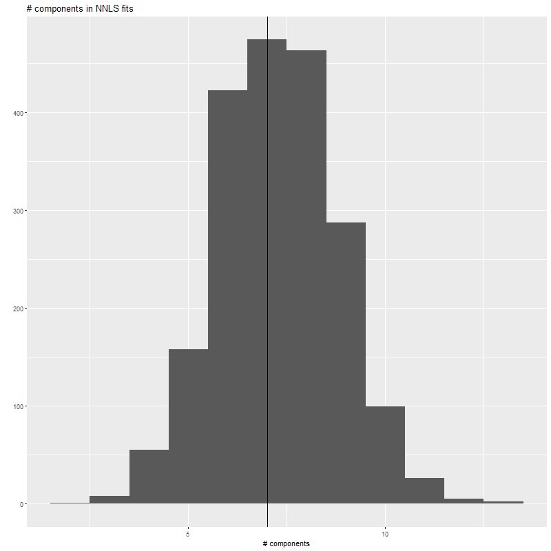
qplot(nnfits$simdat$nnzero,geom='histogram',binwidth=1) +
geom_vline(xintercept=median(nnfits$simdat$nnzero)) +
xlab("# components")+ggtitle("# components in NNLS fits")
table(nnfits$simdat$nnzero)
## simulate not so many calls to DEoptim. This also takes a while...
system.time(defits <- sim_de(X, y_act, sdev=sdev, N=100))
x11()
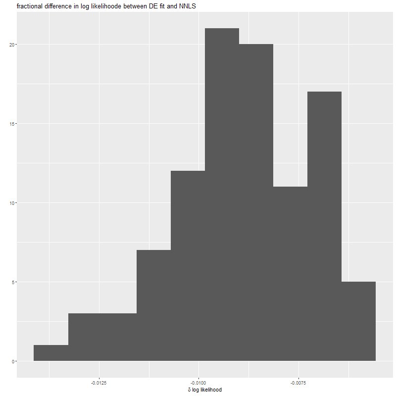
qplot(defits$simdat$deltall,geom='histogram',bins=10) +
xlab(expression(paste(delta~"log likelihood"))) +
ggtitle("fractional difference in log likelihood between DE fit and NNLS")
The function sim_nn is in the file toynnutils.r. This just generates N randomly perturbed sets of the observation vector y, fits them using nnls, and returns some information about the fits (in Windows the CPU time estimates will be not very accurate):
sim_nn <- function(X, y_act, sdev=0.02, N=1000, seed=12345L) {
  require(nnls)

  set.seed(seed)
  nnzero <- numeric(N)
  ctime <- numeric(N)
  ll <- numeric(N)
  nr <- length(y_act)
  nv <- ncol(X)
  B <- matrix(0, N, nv)
  res <- matrix(0, N, nr)
  for (i in 1:N) {
    y <- y_act + rnorm(nr, sd=sdev)
    ctime[i] <- system.time(nnsol <- nnls(X,y))[1]
    B[i,] <- nnsol$x
    nnzero[i] <- nnsol$nsetp
    ll[i] <- sum(dnorm(residuals(nnsol), sd=sdev, log=TRUE))
    res[i, ] <- residuals(nnsol)/sdev
  }
  list(simdat=data.frame(ctime=ctime, nnzero=nnzero, ll=ll), B_nn=B, res_nn=res)
}
The first ggplot2 call in the script produces this histogram of the number of non-negative components of the nnls fits. As expected and consistent with typical real data nnls always returns sparse fits, although almost never quite so sparse as the input. The call to table() returns
Number of nonzero parameter estimates in NNLS fits
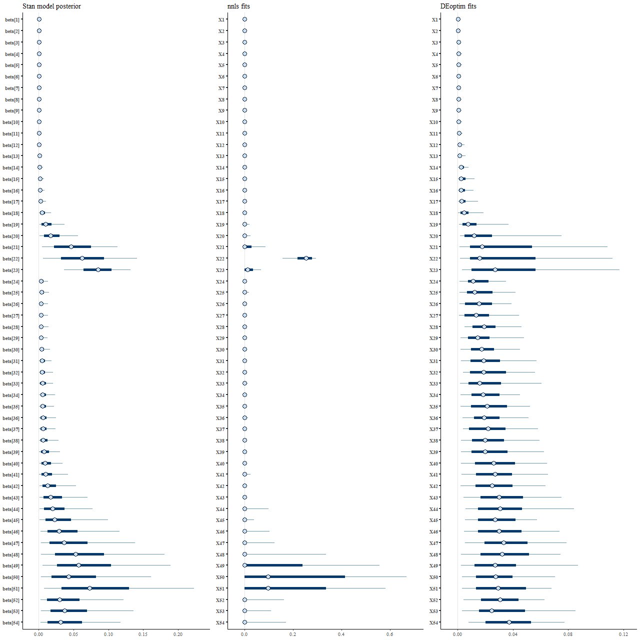
Perhaps the most interesting result of these simulations are the distributions of parameter estimates — these show 50 (thick lines) and 90% (thin lines) intervals, with median values marked by symbols:
Parameter estimates from different fitting methods: (L) posterior distribution from Stan (M) NNLS (R) DEoptim
What’s most striking to me at least is how different the posterior marginal distributions from Stan (left panel) are from the maximum likelihood fits (middle). Star formation is much more extended in time in the Stan model, with both “bursts” replaced with broad ramps up and decays. The Monte Carlo optimization results look superficially similar to the Stan posterior, but as I’ll show soon there are different causes for their behavior.
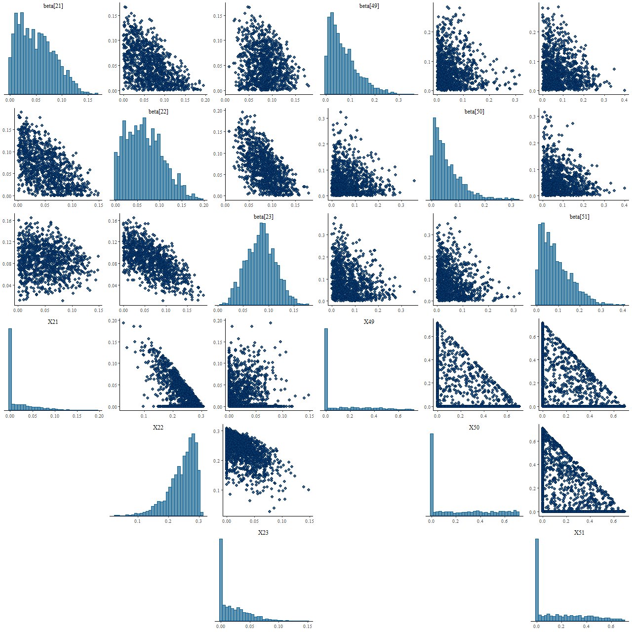
Let’s take a closer look at the distributions of some of the parameter values. This is called a pairs, or sometimes corner, plot — it displays the marginal distribution of each selected parameter along the diagonal and fills out the remaining rows and columns with the joint distributions of pairs of parameters. For this plot I just selected the two non-zero inputs and the surrounding age bins. The top rows are the Stan posterior, the bottom the nnls fits from the 2000 sample simulation.
Pairs plot for selected parameters: (T) Posterior draws from Stan model (B) NNLS estimates
In frequentist statistics a confidence interval is a statement about the behavior of the estimator for a parameter under repeated experiments with the same conditions. It’s not a statement about the parameter itself, which is forever unknowable. A Bayesian confidence interval (to the fussy, credible interval) on the other hand is a statement about the parameter itself.
I’m unaware of any formula for confidence intervals of nnls coefficient estimates, but the simulation we performed gives good numerical estimates of the distribution of parameter values, and these are clearly significantly different from the posterior distributions from Stan. So, not only is there a difference in interpretation between frequentist and Bayesian confidence intervals in this case the values obtained are significantly different as well.
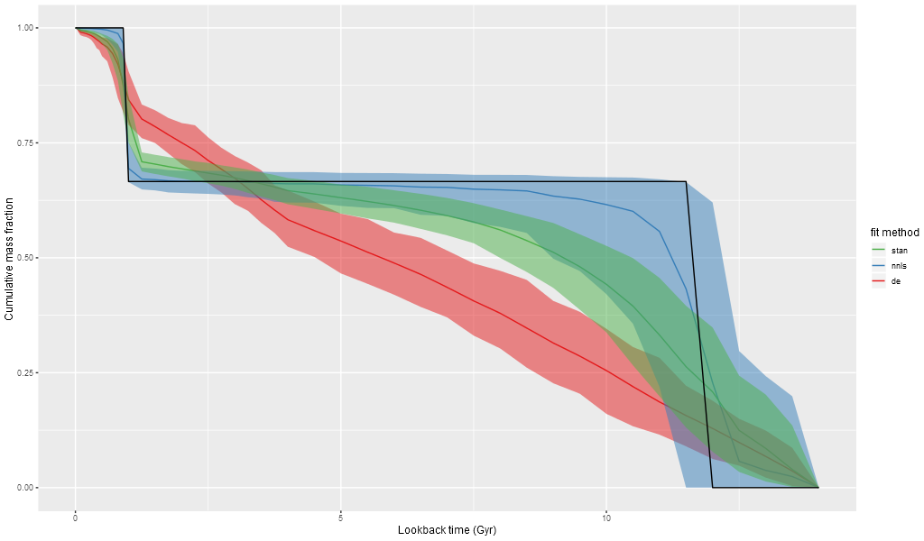
Mass growth histories have become a popular tool for visualizing SFH models, so for fun I created mock histories for the three methods tested here. These show medians and 95% confidence bands. The input MGH just falls within the 95% confidence band of the nnls fits, although the median has more extended mass growth.
Model “mass growth histories” from simple two component input
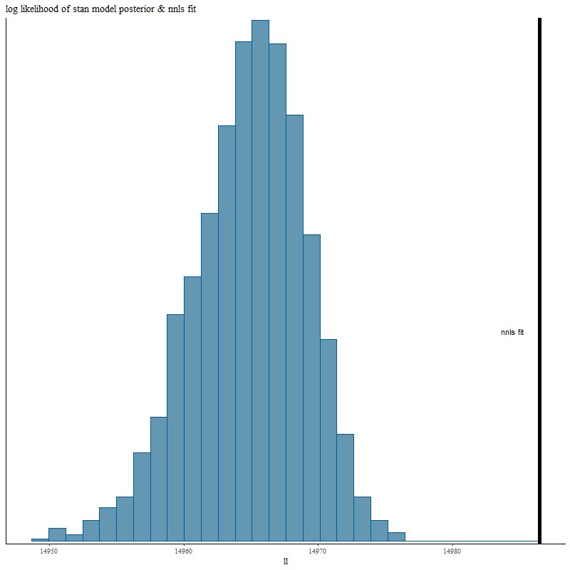
Turning next to fits to the data let’s look first at the overall fits measured by summed log-likelihood. Remember that the nnls solution is the maximum likelihood estimator and therefore neither of the other fitting methods can exceed its log-likelihood for any given realization of the data.
Here’s the posterior log-likelihood from the Stan model run. The vertical line to the right is for the nnls fit. The Stan fit average falls short of the maximum likelihood by about 0.1%. We’ll examine why in more detail next post.
log likelihood of posterior fits
I only ran 100 simulations of the “differential evolution” optimizer because it takes rather a long time (average ~450 sec. per data realization on my PC). The output log-likelihood consistently falls about 1% short of the nnls solution:
fractional δ log likelihood between DEoptim and NNLS fits for 100 data realizations
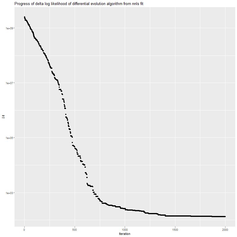
This shows the progress of the optimizer for a single data realization. Progress is rapid at first, but it slows down as it gets close to the optimum and can stall out for many iterations. This algorithm has a hard time getting to a sparse solution.
Progress of DEoptim fits (difference in log likelihood with NNLS fit)
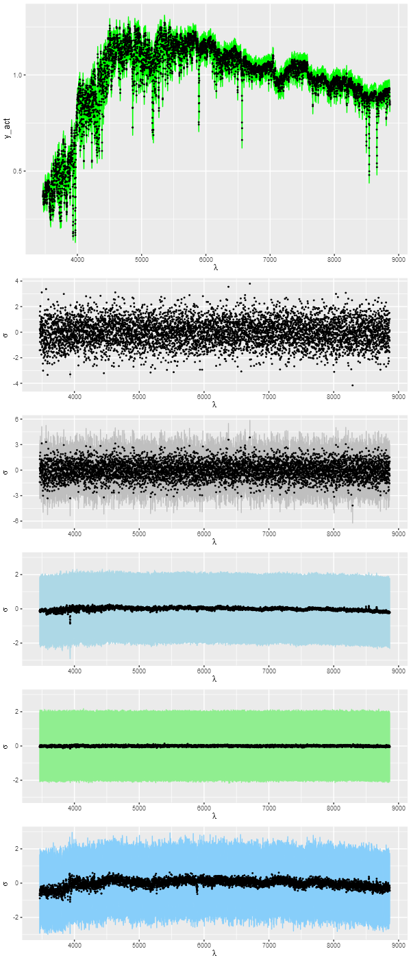
Next let’s look at detailed fits to the data. The top pane shows the unperturbed spectrum (black points) and a 95% confidence band for the posterior predictive fit (green ribbon) from the Stan model. What’s that? Simple: take parameter draws from the posterior and generate new data according to the model. This is done with the following lines in the generated quantities block of the Stan code:
It turns out that the 95% confidence band covers 100% of the true, unperturbed, spectral values and 95% of the perturbed ones, which indicates a successful model.
The remaining panes show several sets of normalized residuals. The first surprised me a bit at first: this shows the residuals (observed – model) of the Stan model posterior. The “points” in this plot are actually error bars — it turns out the range of residuals at any wavelength is rather small (I naively expected that residuals at each point would vary randomly around 0). The residuals from the posterior predictive fits shown in the next panel do show this behavior. This and the remaining panels display median values as points and 95% confidence bands.
The 4th pane shows the errors in the posterior predictive fits, that is the original unperturbed data minus the posterior predictive values. There are hints of systematics here: a bit of curvature at the red and blue ends of the spectrum and a few absorption lines are slightly misfit.
The final two are residuals from the simulated nnls and Monte Carlo optimization fits. The nnls fits have exactly the expected statistical behavior while the latter clearly struggles to fit the data. This is because the overly extended star formation histories reached in the number of iterations allotted result in stellar temperature distributions that aren’t quite right, affecting both the continuum and many absorption features.
Fits to data: T) input spectrum and posterior predictive fit from Stan model 2) Residuals from Stan model posterior 3) Residuals from posterior predictive fits 4) Errors from posterior predictive fits 5) Residuals from NNLS fits 6) Residuals from DEoptim fits
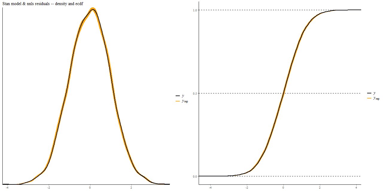
Finally, here is a comparison of the distribution of the residuals in the Stan fit to the same data realization fit by nnls, the colored bands being the former. These show kernel smoothed density estimates on the left and empirical CDF on the right.
Comparison of distribution of residuals in Stan model fit with nnls fit
It’s sometimes suggested in the SFH modeling literature to get parameter uncertainty estimates by randomly perturbing data and refitting it. This is a computationally viable strategy with a competent non-negative least squares solver, but as we saw above this is likely to produce very different estimates than a proper Bayesian analysis.