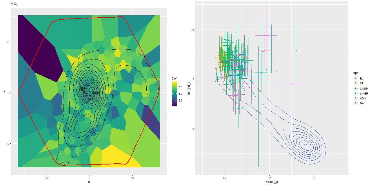
I’ve mentioned a few times that I took a shot several years ago at selecting a sample of post-starburst, or to use a term that’s gained some currency recently, “transitioning” galaxies1transitioning in this context implies that star formation has recently ceased or is in the process of shutting down. To cite one example Alatalo et al. (2017) use the word 18 times with this meaning. One thing that astronomers have come to realize is that traditional K+A spectroscopic selection criteria (basically requiring a combination of strong Balmer absorption lines and weak emission) potentially miss important populations, for example galaxies hosting an AGN. Selecting for weak emission also implies that star formation has already shut down, which precludes finding galaxies that are in the process of shutting down but still forming stars. On the other hand simply dropping constraints on emission won’t work because the resulting sample would be contaminated with a large fraction of normal star forming galaxies. Here is a popular spectroscopic diagnostic diagram, plotting the (pseudo) Lick HδA index against the 4000Å break strength index Dn(4000). This version used the MPA-JHU measurements for approximately 1/2 of SDSS single fiber galaxy spectra from DR8.
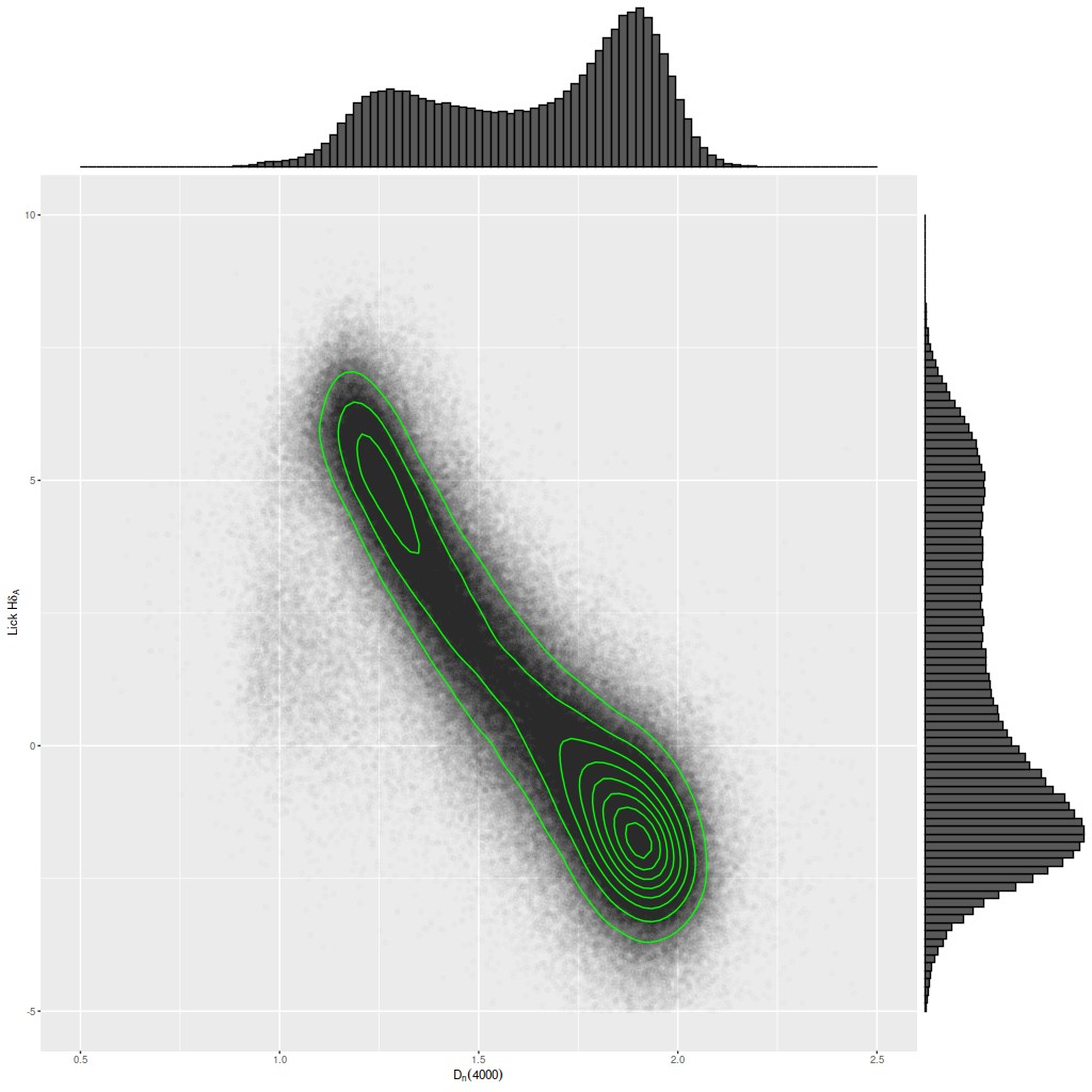
As is true of many observed properties of galaxies the distribution in this diagram is strongly bimodal, with one of the modes centered right around HδA ≈ 5Å. For the most part this region of the Hδ-D4000 plane is occupied by starforming galaxies — somewhere around 8-10% of all SDSS spectra with MPA measurements have HδA ≥ 5Å, while true K+A galaxies are no more than a fraction of a percent of the local population. I took the simplest possible approach to try to minimize contamination from starforming galaxies: besides a traditional K+A selection with slightly relaxed emission line constraints I made a selection of spectra with emission line ratios in the “other than starforming” region of the [N II]/Hα vs [O III]/Hβ BPT diagnostic. I decided to use Kauffmann’s empirical starforming boundary as the selection criterion, and therefore included the so-called “composite” region of the BPT diagnostic. For the sake of completeness and reproducibility here is part of the CASJobs query I used. I saved a number of measurements from the MPA spectroscopic pipeline as well as the SDSS photo pipeline that aren’t included in the listing below. I did include a few lines just to point out that it’s important to use the emission line subtracted version of the Lick Hδ index because it can be significantly contaminated. Most of the where clause of the query is selecting spectra with firm detections and good error estimates of the relevant emission and absorption lines. There is also a redshift range constraint — the upper limit is set to avoid contamination of Hδ by the 5577Å terrestrial night sky line. Finally there are some modest quality constraints.
select into mydb.kaufpostagn
  gi.lick_hd_a_sub as lick_hd_a,
  gi.lick_hd_a_sub_err as lick_hd_a_err,
  gi.d4000_n,
  gi.d4000_n_err
from specObj s
  left outer join PhotoObj as p on s.bestObjid = p.Objid
  left outer join galSpecline as g on s.specObjid = g.specObjid
  left outer join galSpecIndx as gi on s.specObjid = gi.specObjid
  left outer join galSpecExtra as ge on s.specObjid = ge.specObjid
  where
  (g.h_alpha_flux/g.h_alpha_flux_err > 3 and g.h_alpha_flux_err > 0) and
  (g.nii_6584_flux/g.nii_6584_flux_err > 3 and g.nii_6584_flux_err > 0) and
  (g.h_beta_flux/g.h_beta_flux_err > 3 and g.h_beta_flux_err > 0) and
  (g.oiii_flux/g.oiii_flux_err > 3 and g.oiii_flux_err > 0) and
  ((0.61/(log10(g.nii_6584_flux/g.h_alpha_flux)-0.05)+1.3 <
    log10(g.oiii_flux/g.h_beta_flux)) or (log10(g.nii_6584_flux/g.h_alpha_flux)>=0.05)) and
  (gi.lick_hd_a_sub > 5 and gi.lick_hd_a_sub_err > 0) and
  (s.z > .02 and s.z < 0.35) and
  (s.snMedian > 10) and
  (s.zWarning = 0 or s.zWarning = 16)
  order by
  s.plate, s.mjd, s.fiberid
I used a second query to make a more traditional K+A selection. This all could have been done with a single query but the conditions get a bit complicated. These queries run in the DR10 “context”2the data release doesn’t actually matter as long as it’s later than DR7 since the last release the MPA pipeline was run on was DR8. should return 4,235 and 874 hits respectively, with some overlap.
select into mydb.myka
s.ra,
s.dec,
s.plate,
s.mjd,
s.fiberid,
s.specObjid,
from specObj s
left outer join PhotoObj as p on s.bestObjid = p.Objid
left outer join galSpecline as g on s.specObjid = g.specObjid
left outer join galSpecIndx as gi on s.specObjid = gi.specObjid
left outer join galSpecExtra as ge on s.specObjid = ge.specObjid
where
  (g.oii_3729_eqw > -5 and g.oii_3729_eqw_err > 0) and
  (g.h_alpha_eqw >  -5 and g.h_alpha_eqw_err > 0) and
  (gi.lick_hd_a_sub > 5 and gi.lick_hd_a_sub_err > 0) and
  (s.z > .02 and s.z < 0.35) and
  (s.snMedian > 10) and
  (s.zWarning = 0 or s.zWarning = 16)
order by
  s.plate, s.mjd, s.fiberid
I thought at the time based solely on examining SDSS thumbnails that there were rather too many false positives in the form of normal starforming galaxies for the intended purpose of the sample. The choice to include galaxies in Kauffmann’s composite region played some role in this — although even the people responsible for this classification scheme admit now that it’s too simple some galaxies really do have spectra that are composites of starforming regions and AGN. But the more important reason I think is the well known problem that single fiber spectra only cover a portion of most nearby galaxies and galaxy nuclei (which were the intended targets) just aren’t representative of the global properties of galaxies. The SPOGS3an acronym formed somehow from the term “shocked post-starburst galaxy survey.” sample of Alatalo et al. 2016, which has similar aims to my selection but more elaborate selection criteria, has (in my opinion) a similar issue of false positives for the same reason.
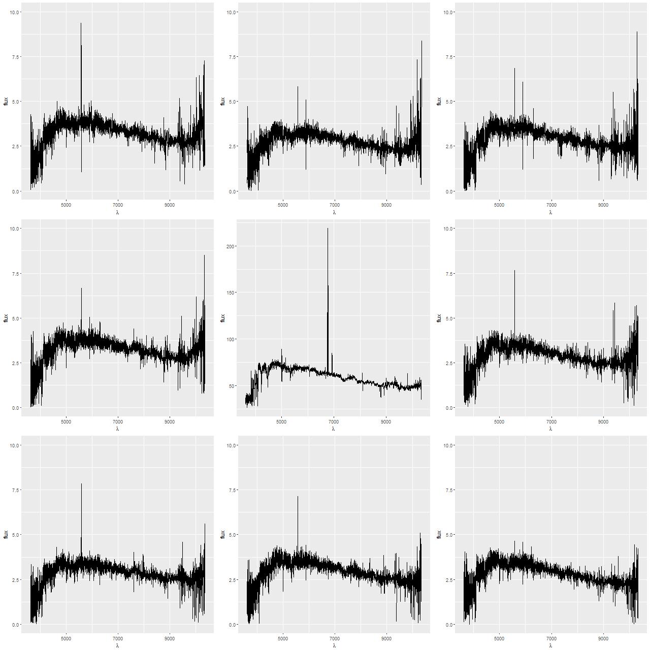
MaNGA provides a unique opportunity to examine the causes of false positives in my transitional sample, and I hope also confirm some real positives. A simple position crossmatch of my sample, which has about 5500 members, with MaNGA DR15 object coordinates produced 29 matches with a position tolerance of about 3″. SDSS thumbnails of the 29 are shown below. By my count at least 13, or 45%, of the sample are visibly disturbed in some way with 7 of those being clear merger remnants with evident shells and tidal tails.
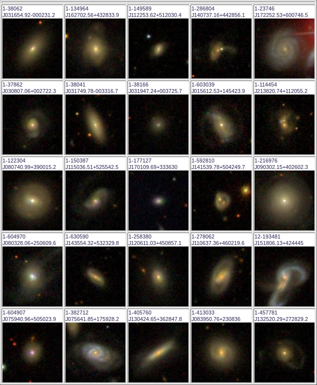
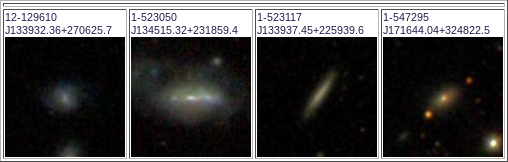
I’ve been calculating star formation history models for these at a leisurely pace and plan to write more about the sample in future posts. Two of these I’ve already written about — besides Mrk 848 number 15 in the postage stamps was the subject of a series of posts starting here. I may write more case studies like those, or perhaps take a more holistic look at the sample and compare to a control group.
As something of an aside, with a looser position matching tolerance a 30th object turns up:
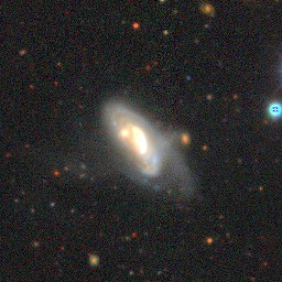
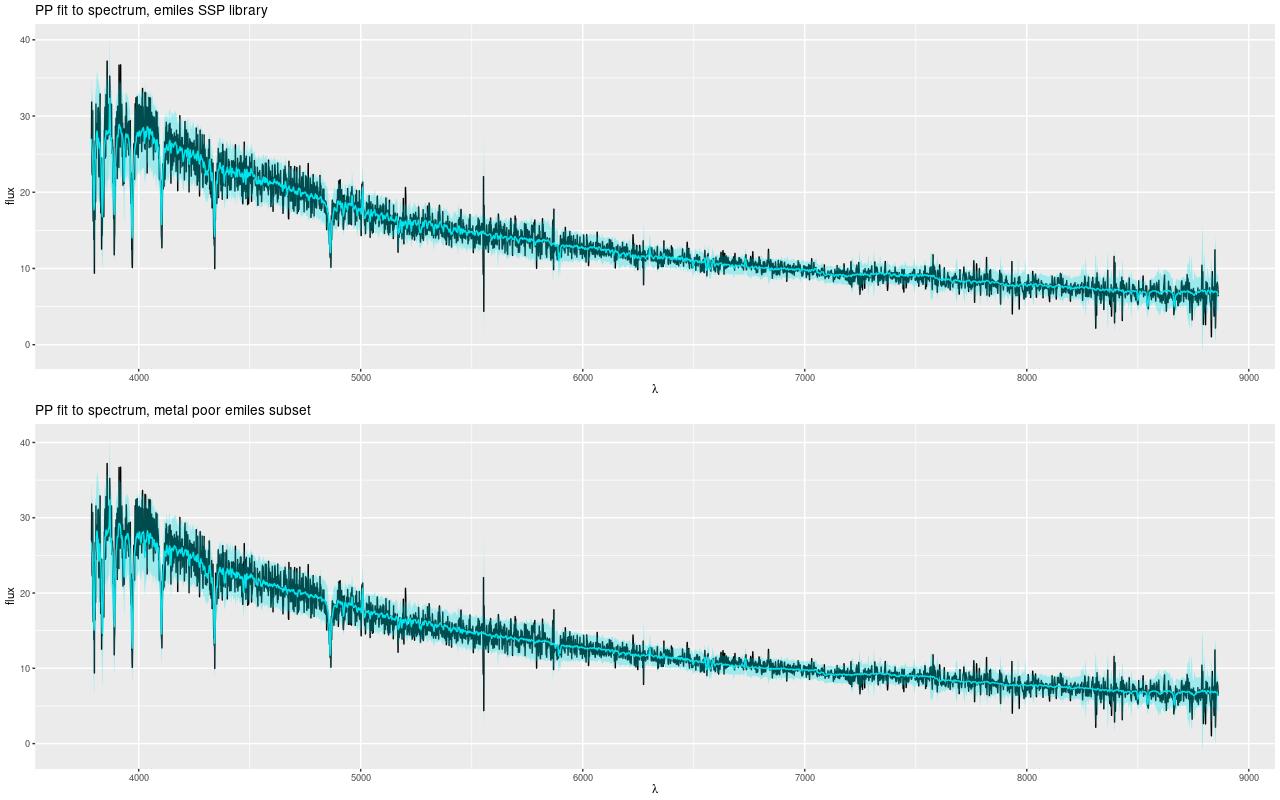
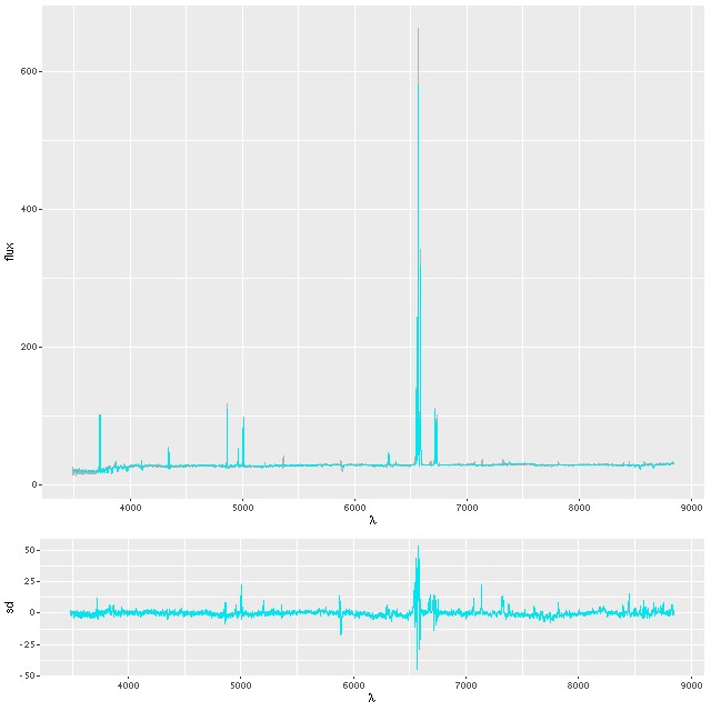
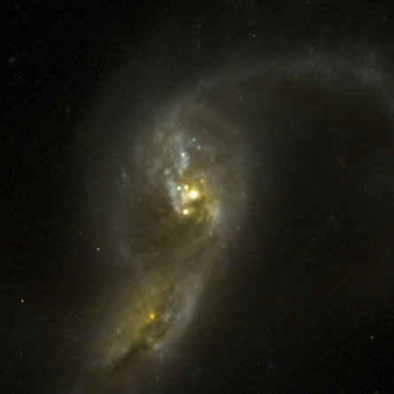
This made my sample based on the spectrum of the eastern nucleus. This object turns out to be doubly strange. Besides having two apparent nuclei, when I did some preliminary spectral fitting I noticed a peculiar pattern of residuals that turned out to be due to this:
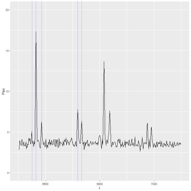
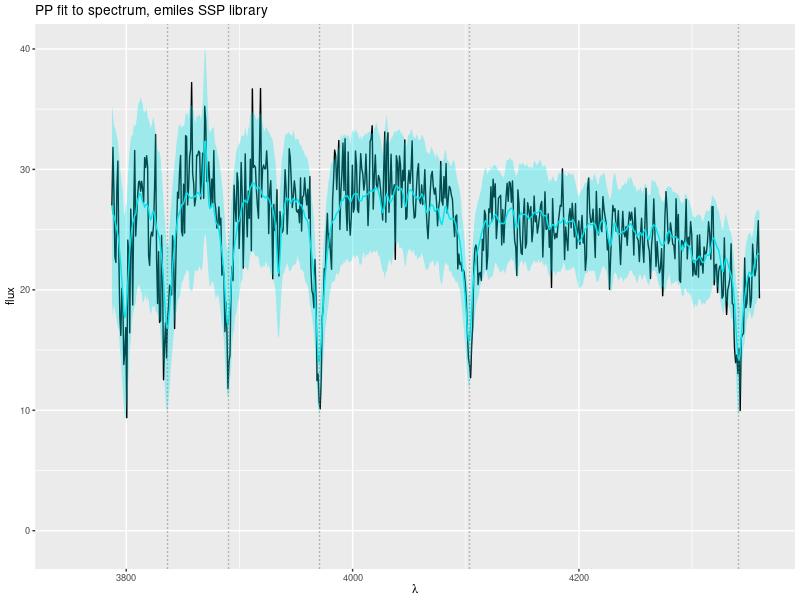
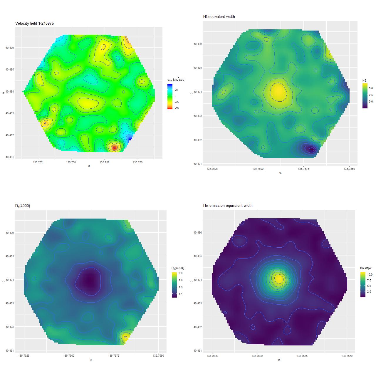
Many of the spectra have emission lines at exactly their rest frame wavelengths. This particular spectrum, which came from somewhere in the SE quadrant of the IFU footprint, clearly shows Hα plus the [N II] and [S II] doublets offset from the same lines at the redshift of the galaxy. It turns out this galaxy lies near the edge of the Orion-Eridanus superbubble, a large region of diffuse emission in our galaxy. Should I choose to study this galaxy in more detail these lines could be masked easily enough, but the metadata for this data cube says it shouldn’t be used.

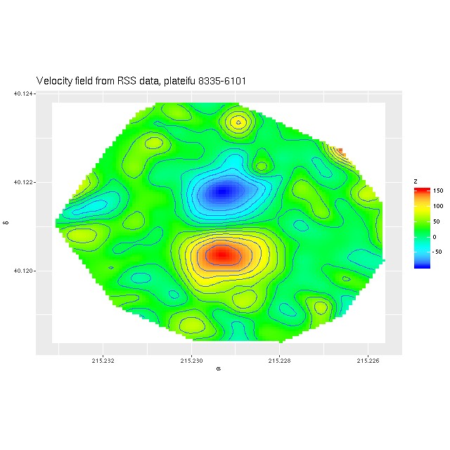 Velocity field estimated from RSS data
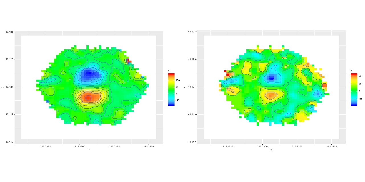 (L) Velocity field estimated for data cube
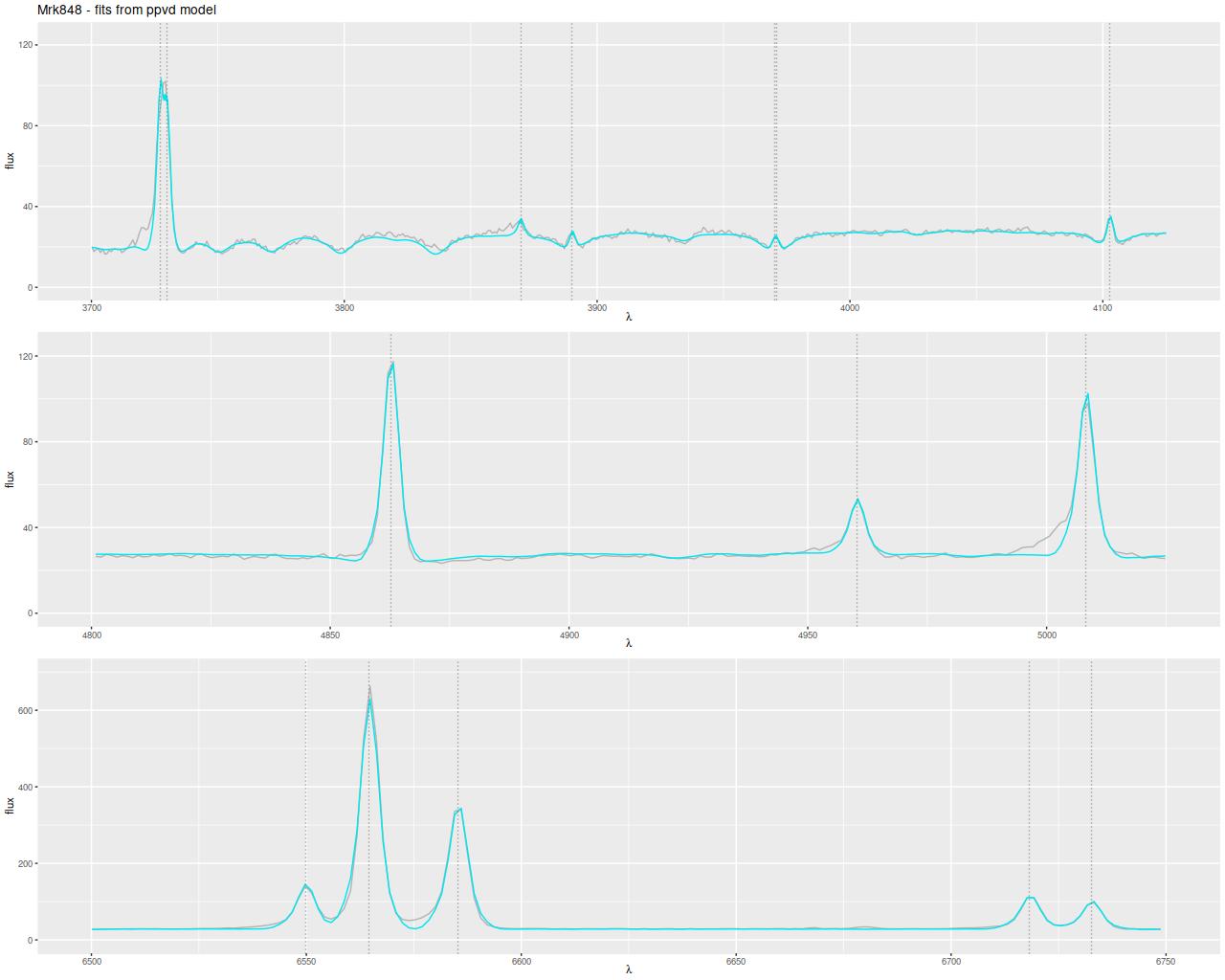
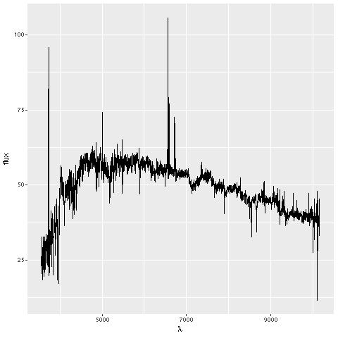 Central fiber spectrum, plateifu 8335-6101
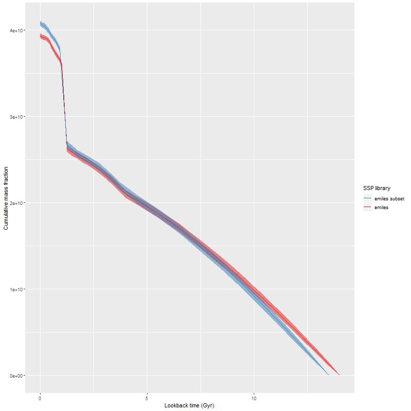
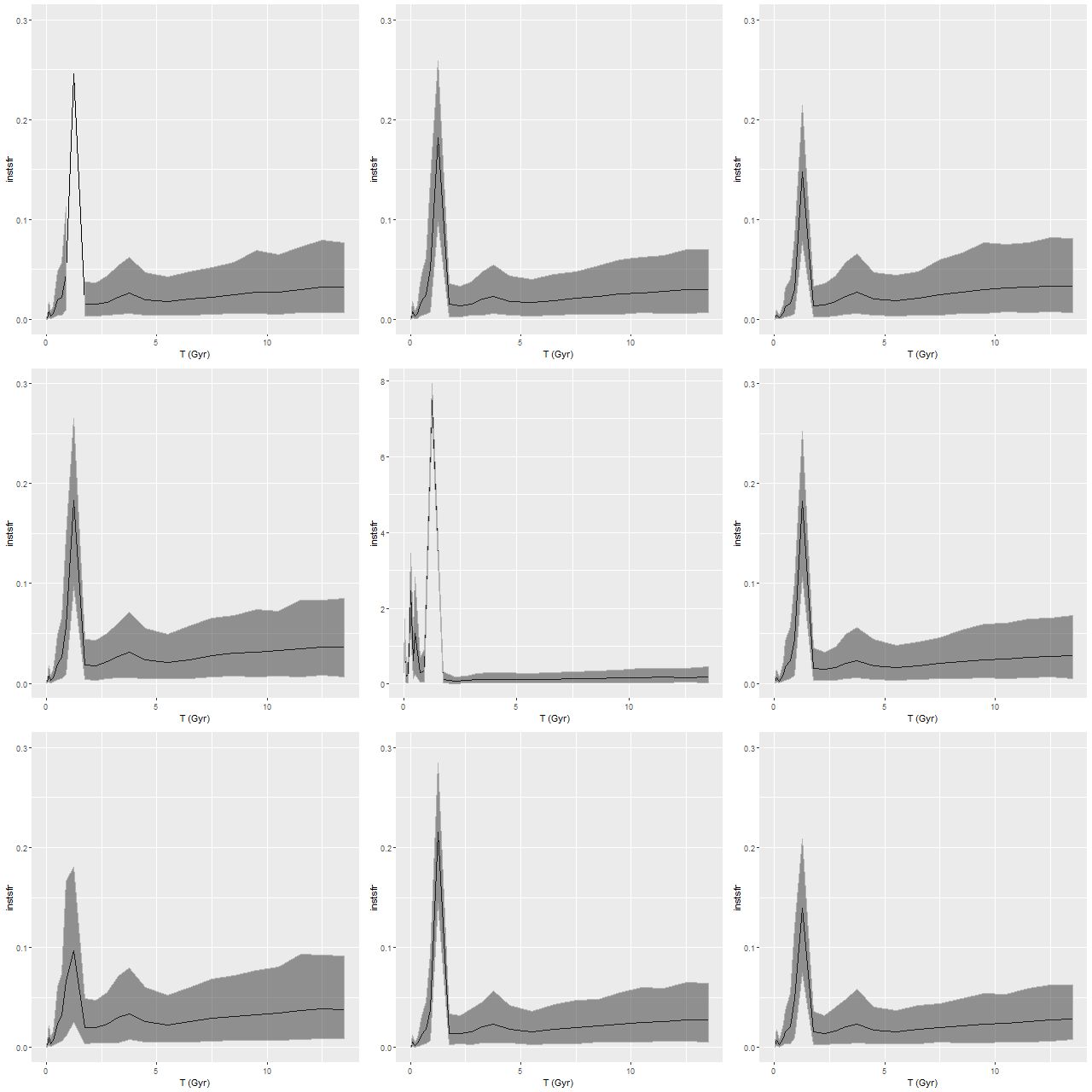
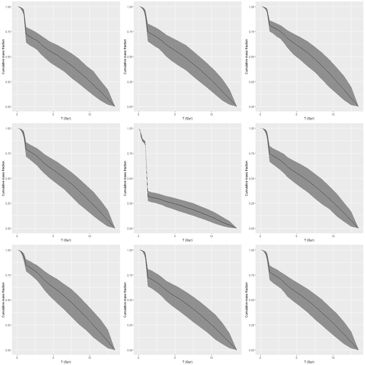
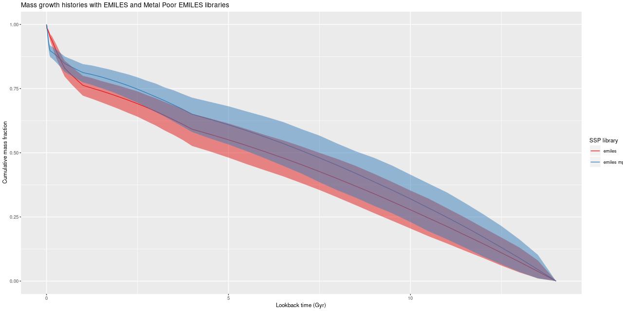
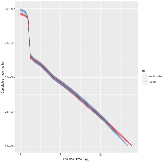 Summed model mass growth histories, emiles subset and “full” emiles
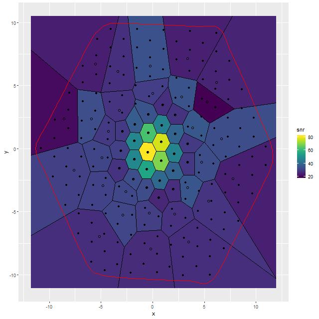
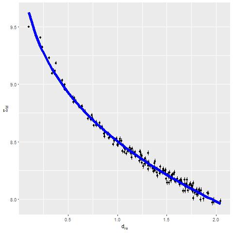
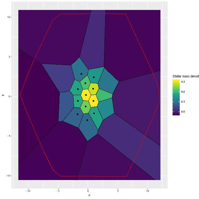 Stellar mass density for binned data, showing outlines of bins and core region
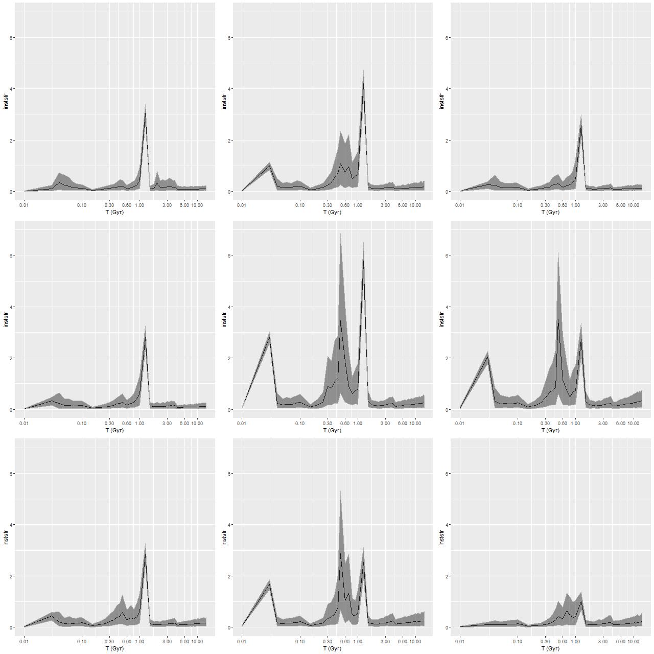
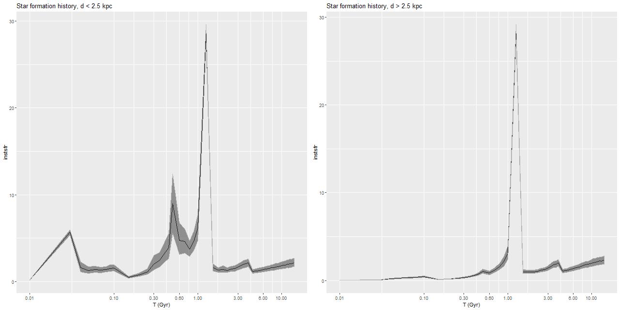
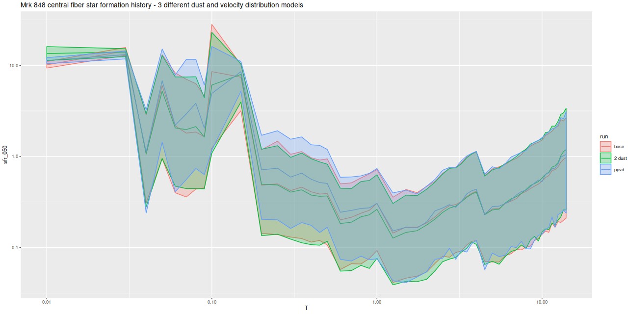
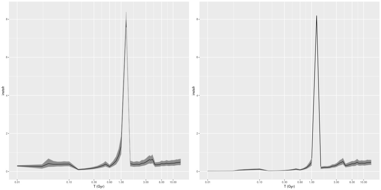 (L) Model Star formation history, inner core
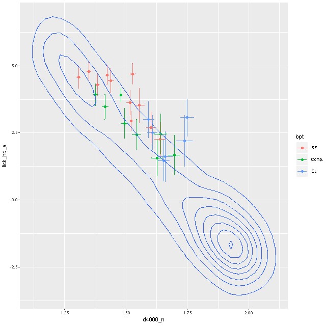 Lick HδA vs. Dn(4000)
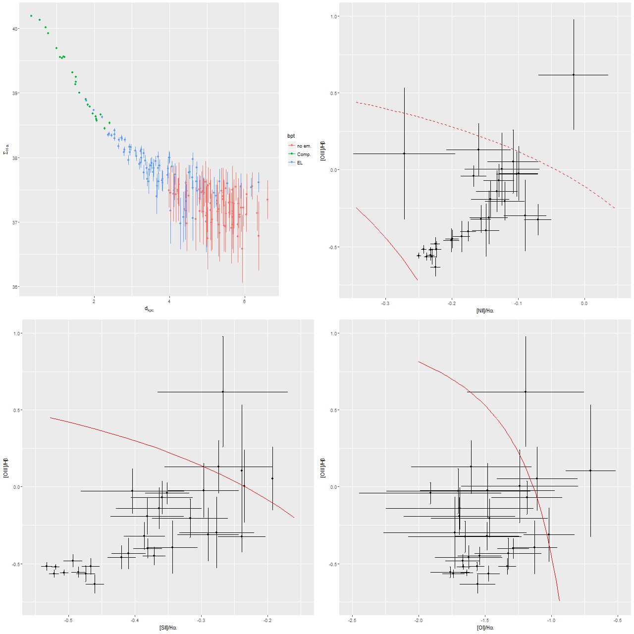
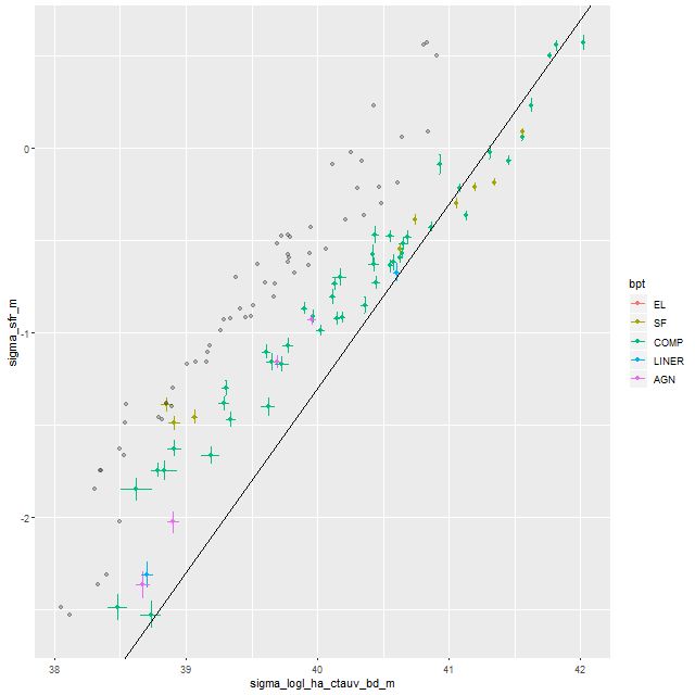
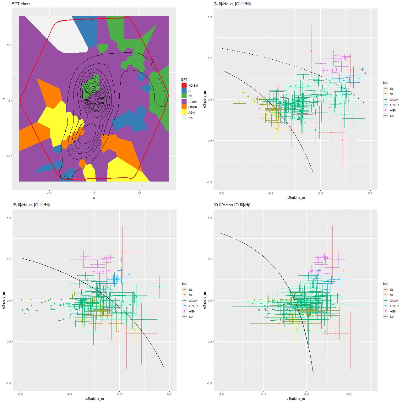
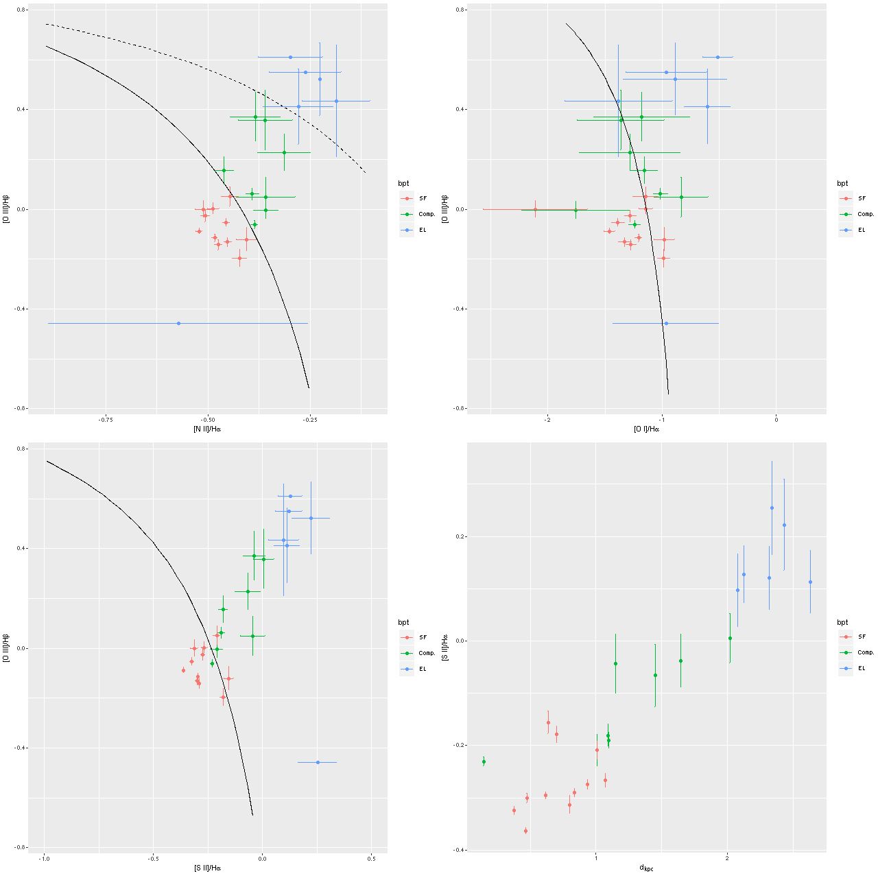 Emission line diagnostic (BPT) plots
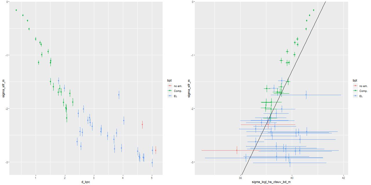
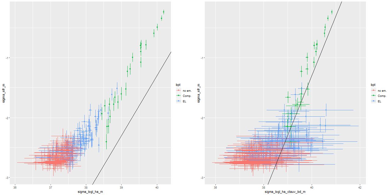
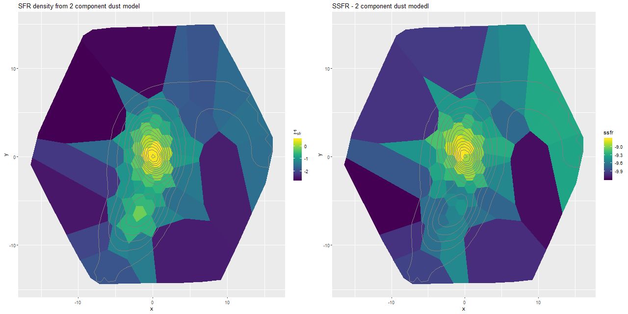
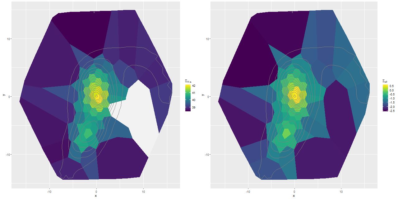
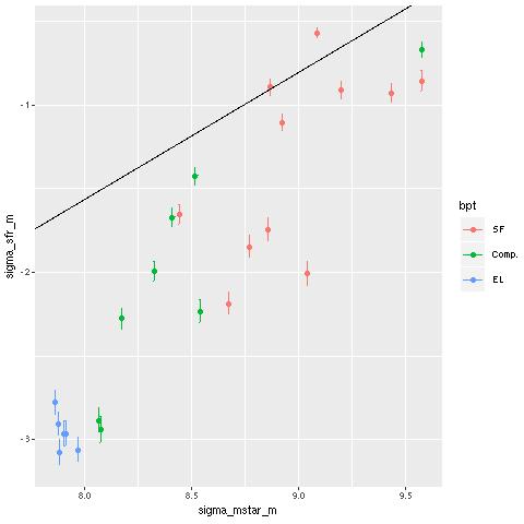 log SFR density vs. log stellar mass density
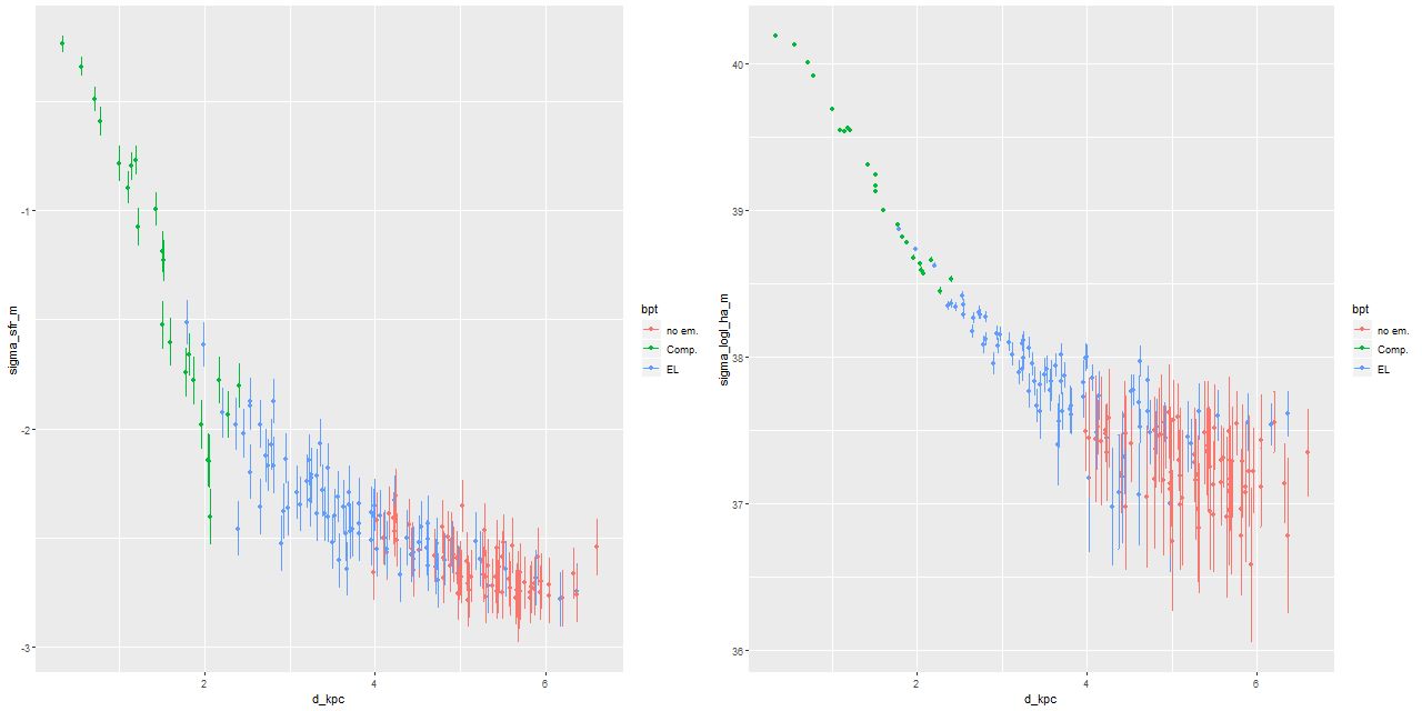
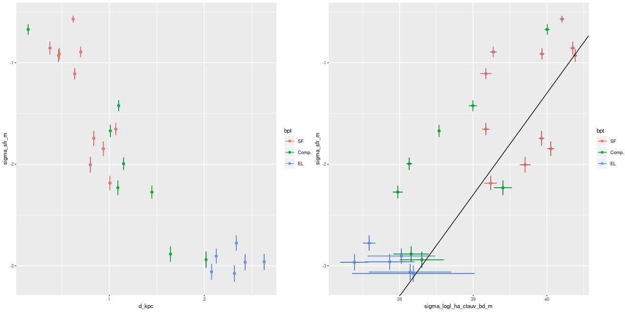 (L) log SFR density vs. radius
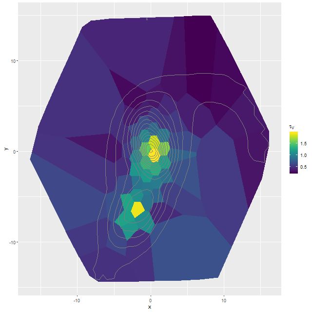
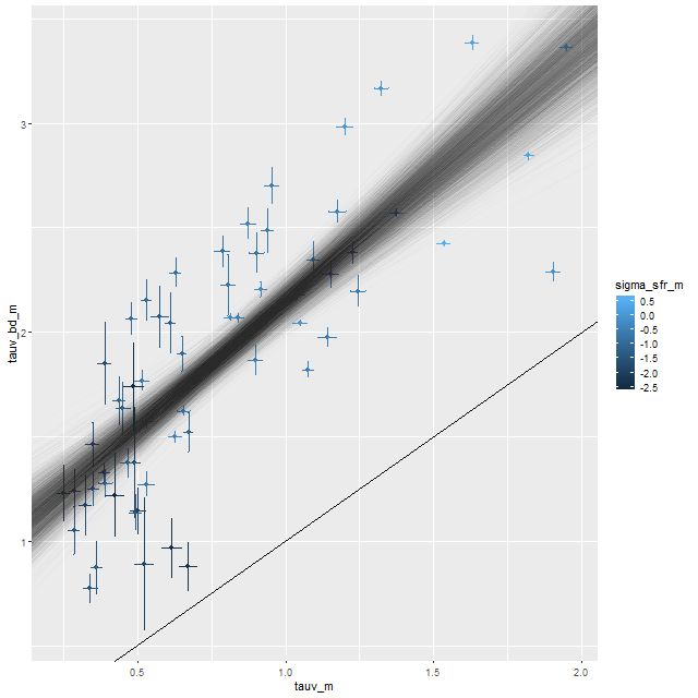
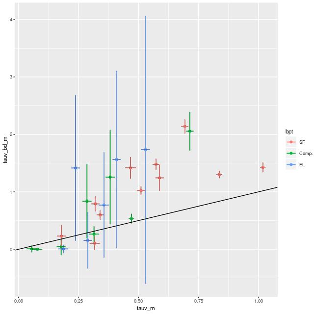 τV estimated from Balmer decrement vs SFH model estimates
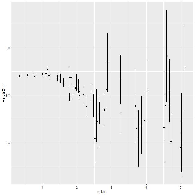
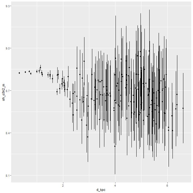
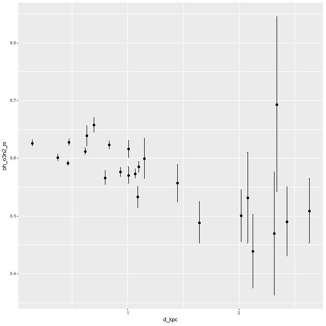 Metallicity 12+log(O/H) vs radius, estimated by O3N2 index