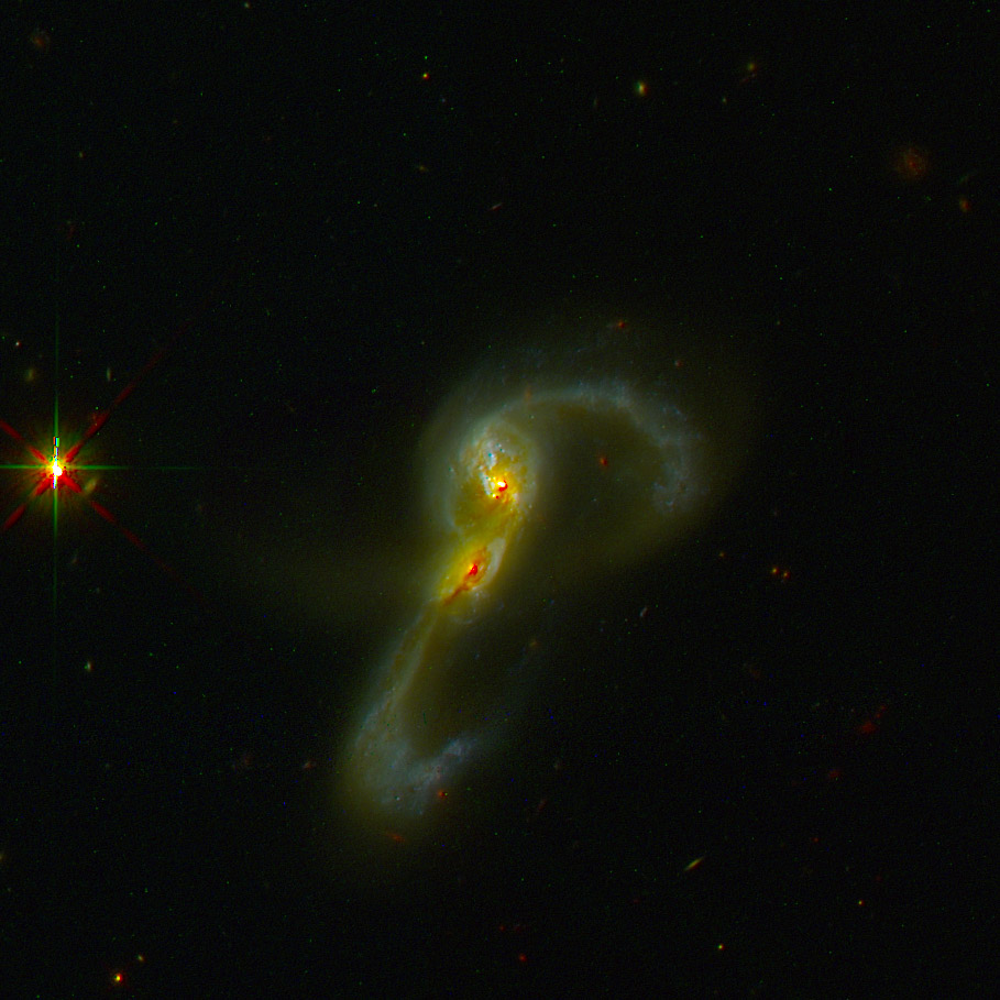
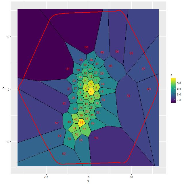
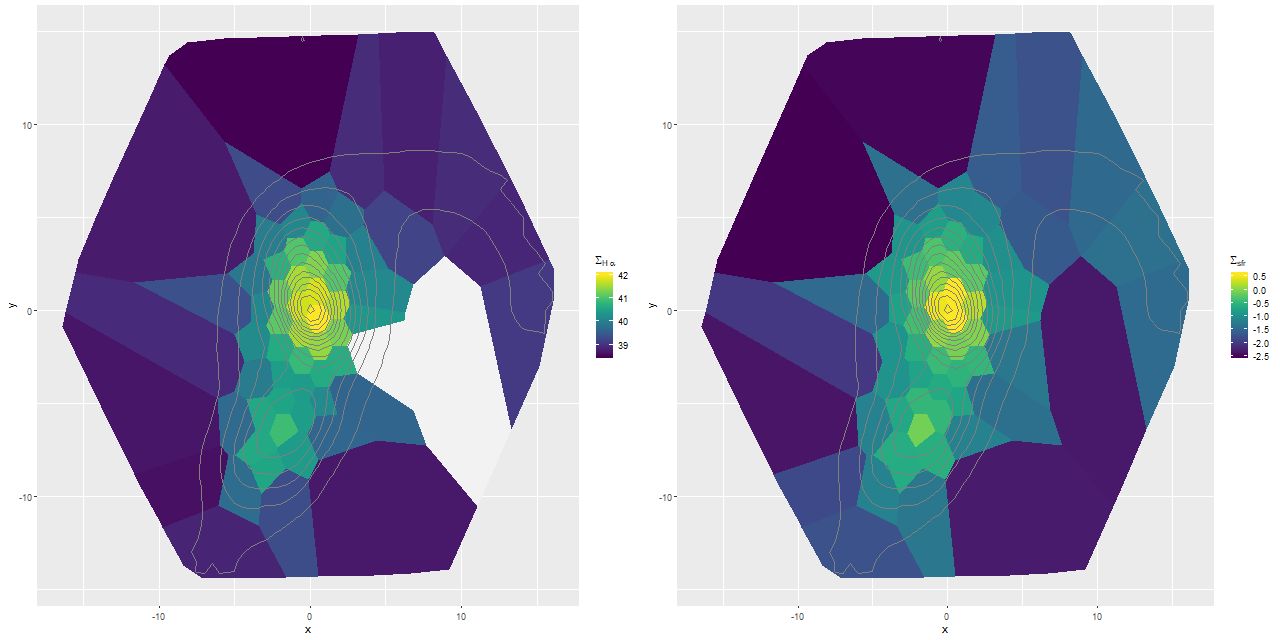
I’m going to close out my analysis of Mrk 848 for now with three topics. First, dust. Like most SED fitting codes mine produces an estimate of the internal attenuation, which I parameterize with τV, the optical depth at V assuming a conventional Calzetti attenuation curve. Before getting into a discussion for context here is a map of the posterior mean estimate for the higher S/N target binning of the data. For reference isophotes of the synthesized r band surface brightness taken from the MaNGA data cube are superimposed:
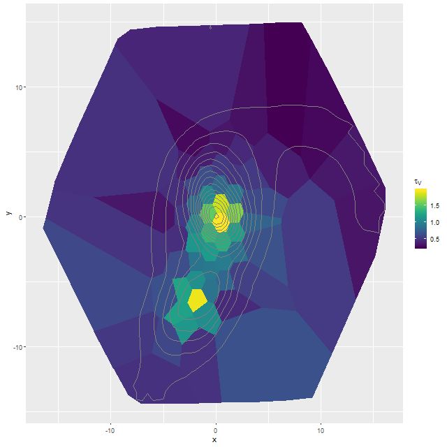
This compares reasonably well with my visual impression of the dust distribution. Both nuclei have very large dust optical depths with a gradual decline outside, while the northern tidal tail has relatively little attenuation.
The paper by Yuan et al. that I looked at last time devoted most of its space to different ways of modeling dust attenuation, ultimately concluding that a two component dust model of the sort advocated by Charlot and Fall (2000) was needed to bring results of full spectral fitting using ppxf on the same MaNGA data as I’ve examined into reasonable agreement with broad band UV-IR SED fits.
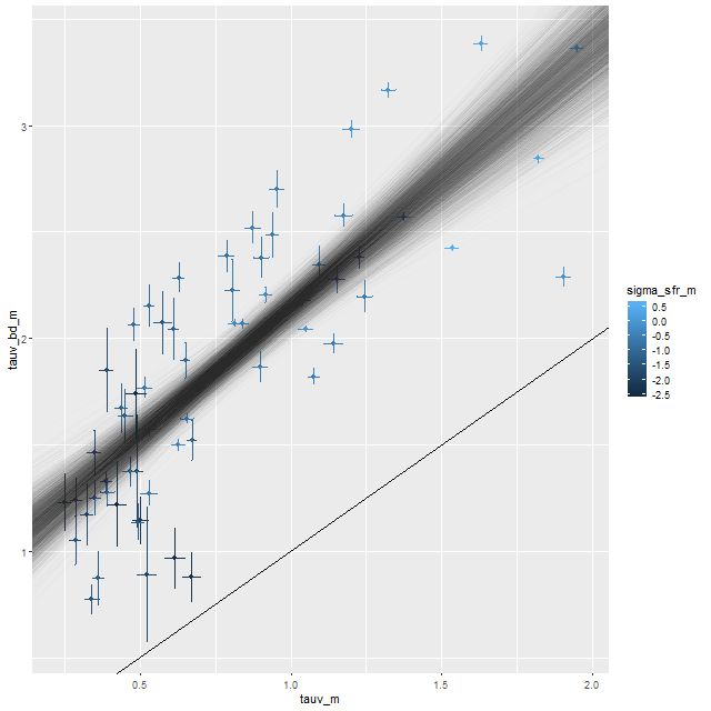
There’s certainly some evidence in support of this. Here is a plot I’ve shown for some other systems of the estimated optical depth of the Balmer emission line emitting regions based on the observed vs. theoretical Balmer decrement (I’ve assumed an intrinsic Hα/Hβ ratio of 2.86 and a Calzetti attenuation relation) plotted against the optical depth estimated from the SFH models, which roughly estimates the amount of reddening needed to fit the SSP model spectra to the observed continuum. In some respects this is a more favorable system than some I’ve looked at because Hβ emission is at measurable levels throughout. On the other hand there is clear evidence that multiple ionization mechanisms are at work, so the assumption of a single canonical value of Hα/Hβ is likely too simple. This might be a partial cause of the scatter in the modeled relationship, but it’s encouraging that there is a strong positive correlation (for those who care, the correlation coefficient between the mean values is 0.8).
The solid line in the graph below is 1:1. The semi-transparent cloud of lines are the sampled relationships from a Bayesian errors in variables regression model. The mean (and marginal 1σ uncertainty) is \(\tau_{V, bd} = (0.94\pm 0.11) + (1.21 \pm 0.12) \tau_V\). So the estimated relationship is just a little steeper than 1:1 but with an offset of about 1, which is a little different from the Charlot & Fall model and from what Yuan et al. found, where the youngest stellar component has about 2-3 times the dust attenuation as the older stellar population. I’ve seen a similar not so steep relationship in every system I’ve looked at and don’t know why it differs from what is typically assumed. I may look into it some day.
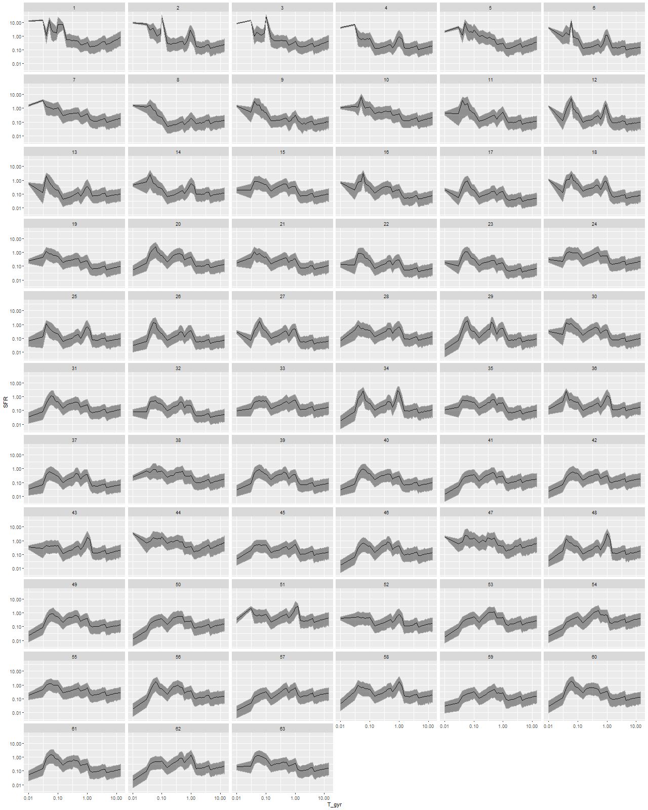
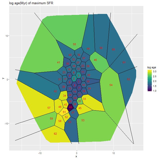
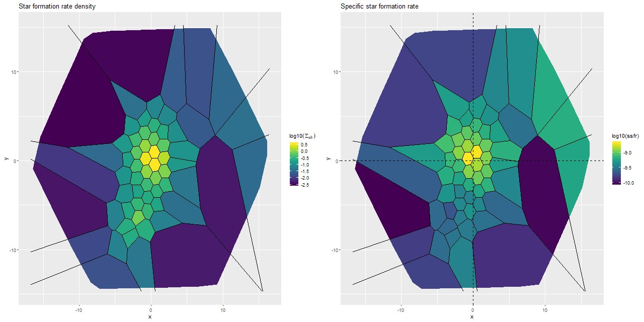
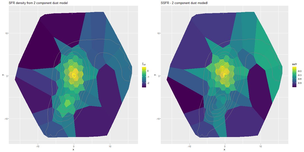
I did have time to run some 2 dust component SFH models. This is a very simple extension of the single component models: a single optical depth is applied to all SSP spectra. A second component with the optical depth fixed at 1 larger than the bulk value is applied only to the youngest model spectra, which recall were taken from unevolved SSPs from the updated BC03 library. I’m just going to show the most basic results from the models for now in the form of maps of the SFR density and specific star formation rate. Compared to the same maps displayed at the end of the last post there is very little difference in spatial variation of these quantities. The main effect of adding more reddened young populations to the model is to replace some of the older light — this is the well known dust-age degeneracy. The average effect was to increase the stellar mass density (by ≈ 0.05 dex overall) while slightly decreasing the 100Myr average SFR (by ≈ 0.04 dex), leading to an average decrease in specific star formation rate of ≈ 0.09 dex. While there are some spatial variations in all of these quantities no qualitative conclusion changes very much.
Contrary to Yuan+ I don’t find a clear need for a 2 component dust model. Without trying to replicate their results I can’t say why exactly we disagree, but I think they erred in aggregating the MaNGA data to the lowest spatial resolution of the broad band photometric data they used, which was 5″ radius. There are clear variations in physical conditions on much smaller scales than this.
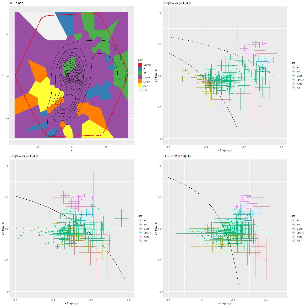
Second topic: the most widely accepted SFR indicator in visual wavelengths is Hα luminosity. Here is another plot I’ve displayed previously: a simple scatterplot of Hα luminosity density against the 100Myr averaged star formation rate density from the SFH models. Luminosity density is corrected for attenuation estimated from the Balmer decrement and for comparison the light gray points are the uncorrected values. Points are color coded by BPT class determined in the usual manner. The straight line is the Hα – SFR calibration of Moustakas et al. (2006), which in turn is taken from earlier work by Kennicutt.
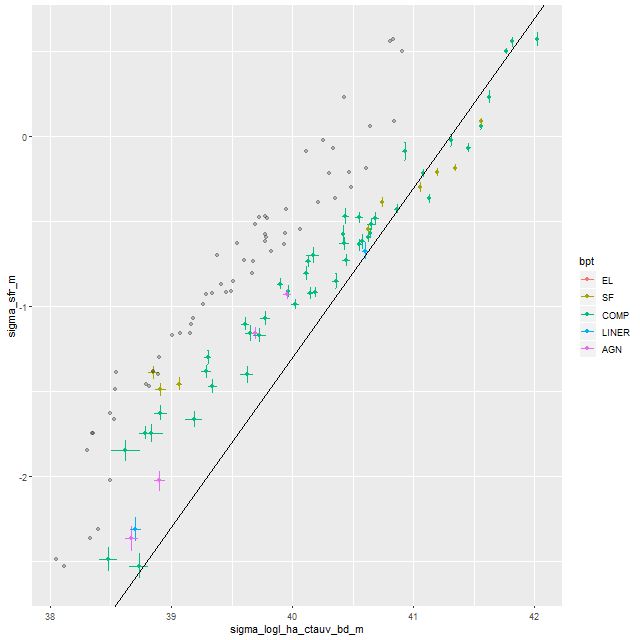
Keeping in mind that Hα emission tracks star formation on timescales of ∼10 Myr1to the extent that ionization is caused by hot young stars. There are evidently multiple ionizing sources in this system, but disentangling their effects seems hard. Note there’s no clear stratification by BPT class in this plot. this graph strongly supports the scenario I outlined in the last post. At the highest Hα luminosities the SFR-Hα trend nicely straddles the Kennicutt-Moustakas calibration, consistent with the finding that the central regions of the two galaxies have had ∼constant or slowly rising star formation rates in the recent past. At lower Hα luminosities the 100Myr average trends consistently above the calibration line, implying a recent fading of star formation.
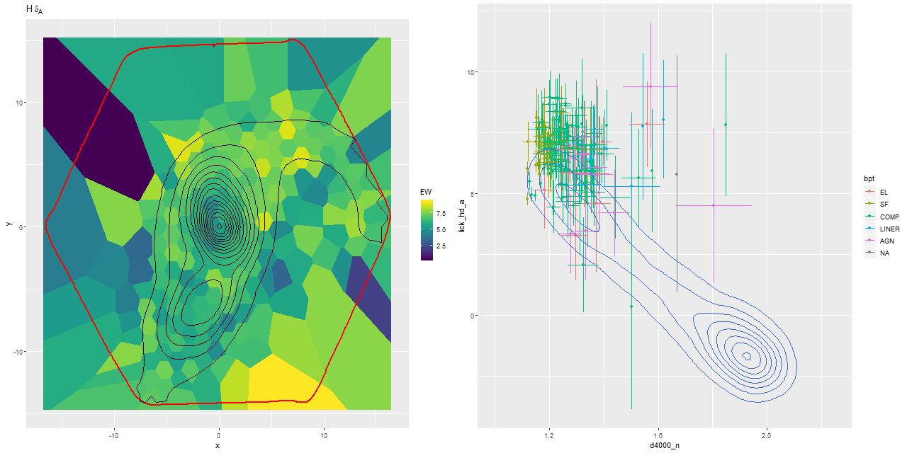
The maps below add some detail, and here the perceptual uniformity of the viridis color palette really helps. If star formation exactly tracked Hα luminosity these two maps would look the same. Instead the northern tidal tail in particular and the small piece of the southern one within the IFU footprint are underluminous in Hα, again implying a recent fading of star formation in the peripheries.
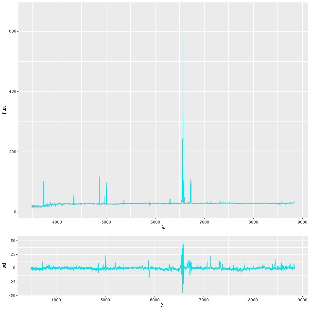
Final topic: the fit to the data, and in particular the emission lines. As I’ve mentioned previously I fit the stellar contribution and emission lines simultaneously, generally assuming separate single component gaussian velocity dispersions and a common system velocity offset. This works well for most galaxies, but for active galaxies or systems like this one with complex velocity profiles maybe not so much. In particular the northern nuclear region is known to have high velocity outflows in both ionized and neutral gas due presumably to supernova driven winds. I’m just going to look at the central fiber spectrum for now. I haven’t examined the fits in detail, but in general they get better outside the immediate region of the center. First, here is the fit to the data using my standard model. In the top panel the gray line, which mostly can’t be seen, is the observed spectrum. Blue are quantiles of the posterior mean fit — this is actually a ribbon, although its width is too thin to be discernable. The bottom panel are the residuals in standard deviations. Yes, they run as large as ±50σ, with conspicuous problems around all emission lines. There are also a number of usually weak emission lines that I don’t track that are present in this spectrum.
I have a solution for cases like this which I call partially parametric. I assume the usual Gauss-Hermite form for the emission lines (as in, for example, ppxf) while the stellar velocity distribution is modeled with a convolution kernel2I think I’ve discussed this previously but I’m too lazy to check right now. If I haven’t I’ll post about it someday. Unfortunately the Stan implementation of this model takes at least an order of magnitude longer to execute than my standard one, which makes its wholesale use prohibitively expensive. It does materially improve the fit to this spectrum although there are still problems with the stronger emission lines. Let’s zoom in on a few crucial regions of the spectrum:
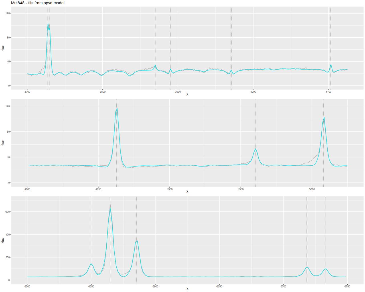
The two things that are evident here are the clear sign of outflow in the forbidden emission lines, particularly [O III] and [N II], while the Balmer lines are relatively more symmetrical as are the [S II] doublet at 6717, 6730Å. The existence of rather significant residuals is likely because emission is coming from at least two physically distinct regions while the fit to the data is mostly driven by Hα, which as usual is the strongest emission line. The fit captures the emission line cores in the high order Balmer lines rather well and also the absorption lines on the blue side of the 4000Å break except for the region around the [Ne III] line at 3869Å.
I’m mostly interested in star formation histories, and it’s important to see what differences are present. Here is a comparison of three models: my standard one, the two dust component model, and the partially parametric velocity dispersion model:
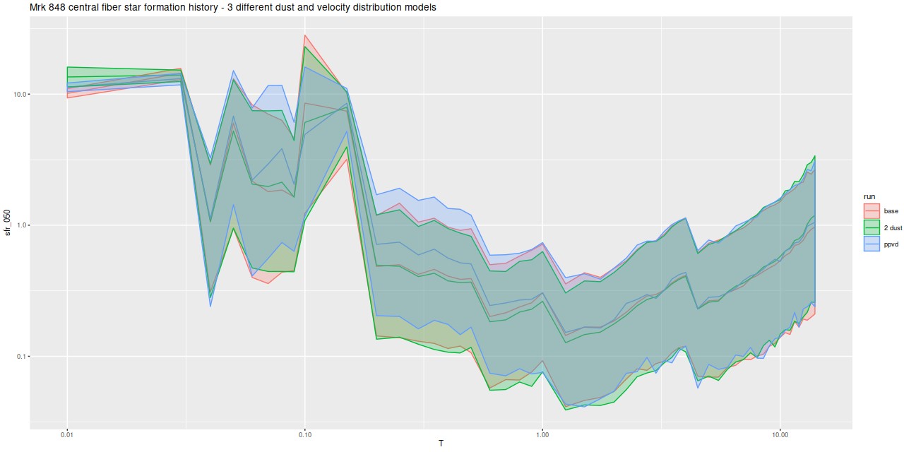
In fact the differences are small and not clearly outside the range of normal MCMC variability. The two dust model slightly increases the contribution of the youngest stellar component at the expense of slightly older contributors. All three have the presumably artifactual uptick in SFR at 4Gyr and very similar estimated histories for ages >1 Gyr.
I still envision a number of future model refinements. The current version of the official data analysis pipeline tracks several more emission lines than I do at present and has updated wavelengths that may be more accurate than the ones from the SDSS spectro pipeline. It might be useful to allow at least two distinct emission line velocity distributions, with for example one for recombination lines and one for forbidden. Unfortunately the computational expense of this sort of generalization at present is prohibitive.
I’m not impressed with the two dust model that I tried, but there may still be useful refinements to the attenuation model to be made. A more flexible form of the Calzetti relation might be useful for example3there is recent relevant literature on this topic that I’m again too lazy to look up.
My initial impression of this system was that it was a clear false positive that was selected mostly because of a spurious BPT classification. On further reflection with MaNGA data available it’s not so clear. A slight surprise is the strong Balmer absorption virtually throughout the system with evidence for a recent shut down of star formation in the tidal tails. A popular scenario for the formation of K+A galaxies through major mergers is that they experience a centrally concentrated starburst after coalescence which, once the dust clears and assuming that some feedback mechanism shuts off star formation leads to a period of up to a Gyr or so with a classic K+A signature4I previously cited Bekki et al. 2005, who examine this scenario in considerable detail.Capturing a merger in the instant before final coalescence provides important clues about this process.
To the best of my knowledge there have been no attempts at dynamical modeling of this particular system. There is now reasonably good kinematic information for the region covered by the MaNGA IFU, and there is good photometric data from both HST and several imaging surveys. Together these make detailed dynamical modeling technically feasible. It would be interesting if star formation histories could further constrain such models. Being aware of the multiple “degeneracies” between stellar age and other physical properties I’m not highly confident, but it seems provocative that we can apparently identify distinct stages in the evolutionary history of this system.