Early type galaxies – Page 2

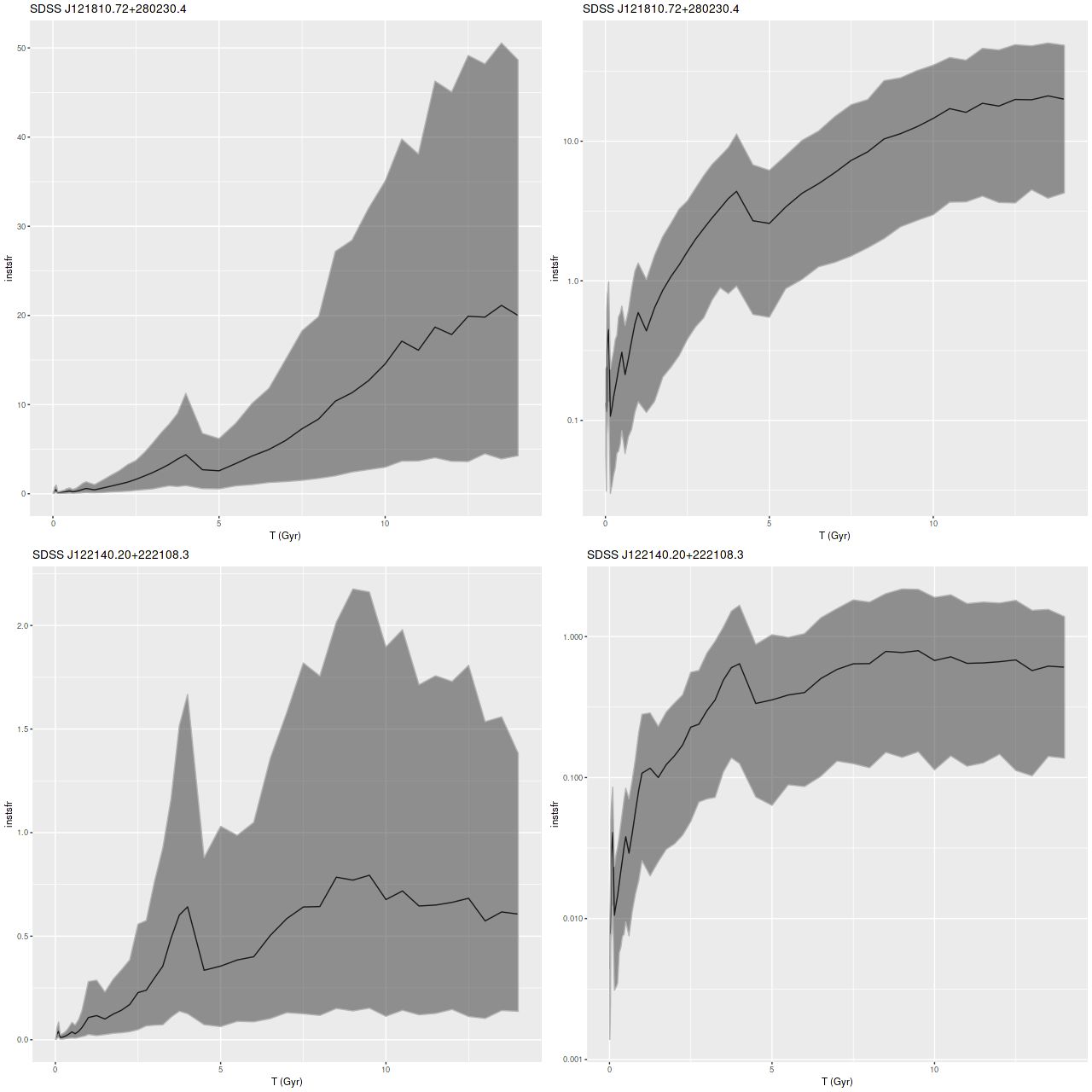
One of my favorite visualization tools for displaying results of star formation history modeling is a ribbon plot of star formation rate versus look back time. This simply plots the marginal posterior mean or median SFR along with 2.5 and 97.5th percentiles (by default) as the lower and upper boundaries of the ribbon. I’ve been using the simplest possible definition of the star formation rate, namely the total mass born in each age bin divided by the interval between the nominal age of each SSP model and the next younger. One striking feature of these plots that’s especially evident in grids of SFH models for an entire galaxy like the one shown in my last post is that there are invariably jumps in the SFR at certain specific ages as marked below. This particular example is from a sample of passively evolving Coma cluster galaxies, but the same features are seen regardless of the likely “true” star formation history.

sfrh — Star formation rate history estimate – emiles with BaSTI isochrones

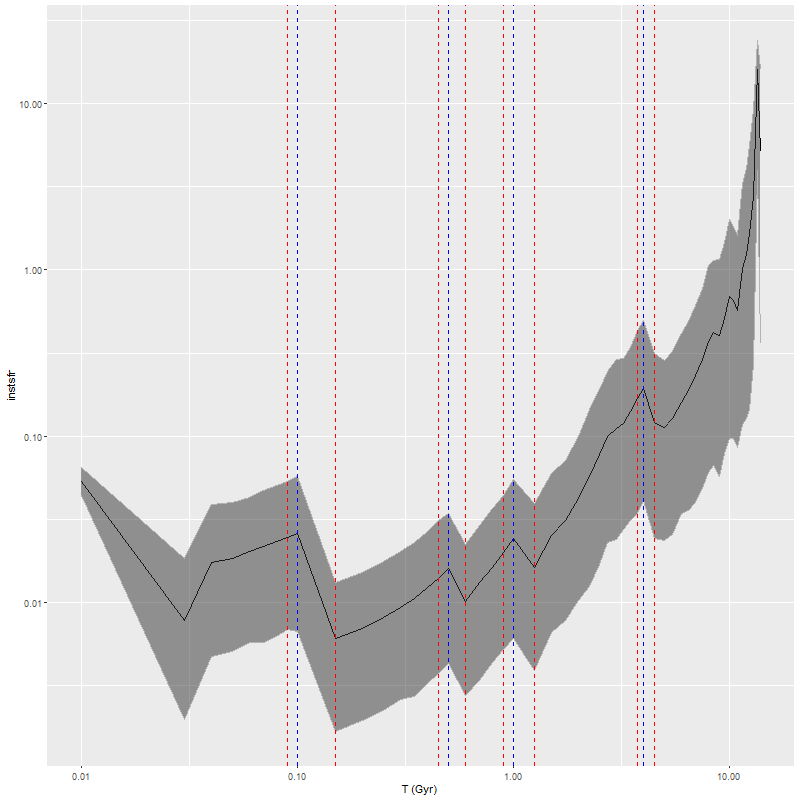
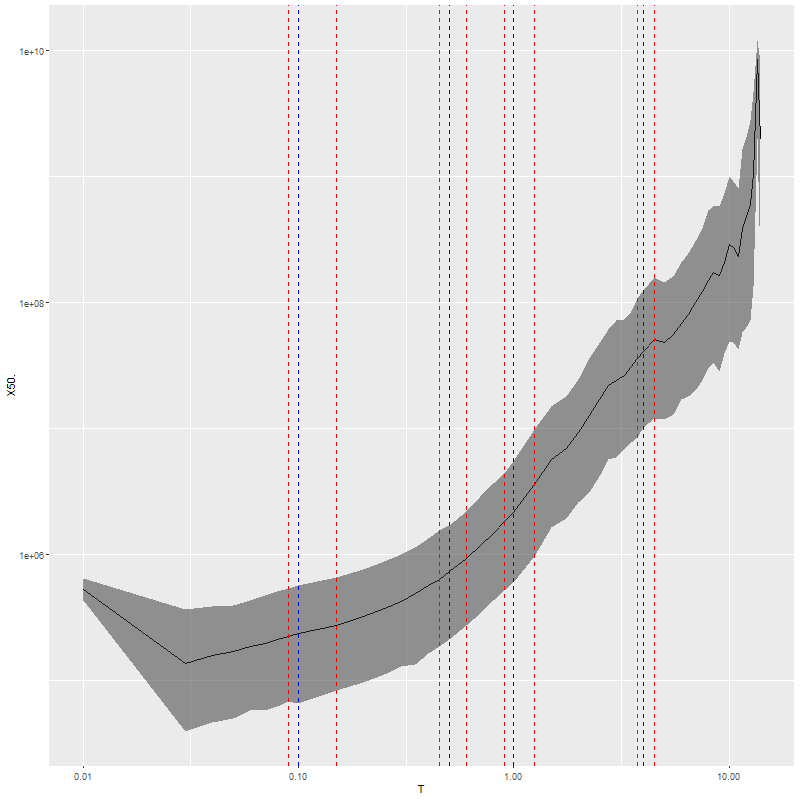
These jumps are artifacts of course: the BaSTI isochrones used for the EMILES SSP models that I currently use are tabulated at age intervals that are constant over certain age ranges, with jumps at 4 ages¹ The jumps in model SFR occur exactly at the breaks in the age intervals. This turns out to be due to an otherwise welcome feature of the SFH models that they “want” to produce SSP contributions that vary smoothly with age as shown below for the same model run. So for example the stellar mass born in the 90-100 Myr age bin per the model is about 90% of that in the 100-150 Myr bin while the time interval increases by a factor of 5, so the model SFR declines by a factor 4.5 or around 0.6 dex.

mass_history — Modeled mass born in each age bin – central spectrum of plateifu 9876-12702

Can I do anything about this? Should I? Changing how I calculate the star formation rate might work — this is after all a derivative and I’m currently using the most stupidly simple numerical approximation possible. It also might help to adjust the effective ages of each SSP model. I should also look at the priors on the SSP model coefficients, although as I noted some time ago it’s hard to affect the model star formation histories much with adjustments to priors.

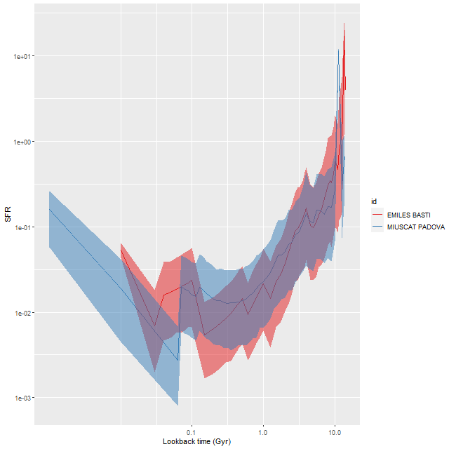
These jumps are something of a peculiarity of the BaSTI isochrones. I had previously used a subset of MILES SSP models from Padova isochrones, which are tabulated at equal logarithmic age intervals. A comparison model run lacks large jumps except for an early time burst. Since the youngest age bin in the Padova isochrones is around 60 Myr I had added two younger SSP models from an update of the BC03 library, and these show abrupt jumps in model SFR. This is also the case with the youngest age bin in my currently used EMILES library.

sfr_compare — Comparison of star formation rate history estimates: Red – EMILES SSP libraries with BaSTI isochrones Blue – Miuscat SSP library with Padova isochrones

A final comment about these visualizations is that often the mode of the posterior distribution of an SSP model contribution is near 0, and it might make sense to display one sided confidence intervals since what we’re really constraining is an upper limit. I may work on this in the future.

This post will be short. Eventually I’d like to add a reproducible real data example or two to the documentation of the software I just officially published. Even though I’m mostly working with MaNGA data these days it may not be practical to include an example since the smallest RSS file is ∼20MB and it can take days to fully process a single data set. The single fiber SDSS spectra on the other hand are only ~170-210KB in “lite” form. While I’m hunting around for suitable examples I’ll post a few results here. For today’s post a couple of randomly selected early type galaxies from my north galactic pole sample:

These don’t seem to be in any historical catalogs, so I’ll just call them by their SDSS designations of J121810.72+280230.4 and J122140.20+222108.3, or J1218+2802 and J1221+2221 for shorthand. The first appears to me to be a garden variety elliptical; the second might be an S0 — neither has a morphological classification listed in NED (a majority of GZ classifiers in both GZ1 and GZ2 called the second an elliptical). Galaxy 2 has a redshift of z=0.023, which puts it in or near the Coma cluster. Galaxy 1 is well in the background at z=0.081.

I modeled the star formation histories with my standard tools and the “full” EMILES ssp library (that is all 54 time bins in 4 metallicity bins). The Stan models both completed without warnings (one required some adjustment of control parameters). Here are some basic results. First, star formation histories, displayed as star formation rate against lookback time. I find it can be useful to use linear or logarithmic scales on either or both axes. Here I show SFR scaled both ways:

sfh_twogalaxies — Star formation histories for 2 passively evolving galaxies

So-called non-parametric models for star formation histories are hoped for gold standards for SFH modeling, and here we see part of the reason: these have rather different estimated mass assembly histories despite similar looking spectra (see below or follow the links), and neither estimate is particularly close to commonly chosen functional forms.

There are some oddities to beware of however. For example literally 100% of the models I’ve run with any variation of the EMILES library show an uptick in mean star formation rate at 4Gyr, independent of the absolute estimated SFR. This can’t be real obviously enough, but I haven’t yet found an error or other specific reason for it. There may be other persistent zigs and zags in SFR at specific times, and these can vary with the SSP library. Overall I assign no particular significance to small variations in mean estimated star formation rates, especially at early times. I’m somewhat more inclined to take seriously late time variations (say, most recent Gyr), which may be wishful thinking.

The data aren’t inconsistent with a small amount of ongoing star formation (estimates of specific star formation rate averaged over 100Myr are shown — these have units of yr^-1). SSFR’s in a range ~10^-11 yr^-1 are about an order of magnitude lower than an ordinary starforming galaxy in the local universe.

ssfr_twogalaxies — froPosterior distribution of specific star formation rate (100 Myr timescale)

Fits to the data are comparable, and satisfactory over most of the wavelength range of the spectra. A recent paper on arxiv (article id 1811.09799) mentioned some fitting issues with EMILES SSP libraries in the red. This can be seen here in the range ~6750-7500Å (rest frame). I don’t have an explanation either. It might be significant that the MILES stellar library spectra extend only to ~7300Å, with other data sources grafted on to the red extension, so there could be a calibration problem. On the other hand the prominent dip in this range is at least partly due to TiO absorption, so this could point to metal abundance variations not captured by EMILES.

Finally, I find it useful to model attenuation, even in ETGs that are often considered dust free. I just use a Calzetti attenuation curve in these models even though it was based on starburst galaxy SEDs and therefore may not be appropriate. This is a topic for possible future model refinement.

tauv_twogalaxies — Posterior estimates of dust attenuation

Category: Early type galaxies

Star formation history modeling and visualization — short note

A random pair of passively evolving galaxies