Early type galaxies – Extragalactic

2023-04-222023-04-22

IC 3025

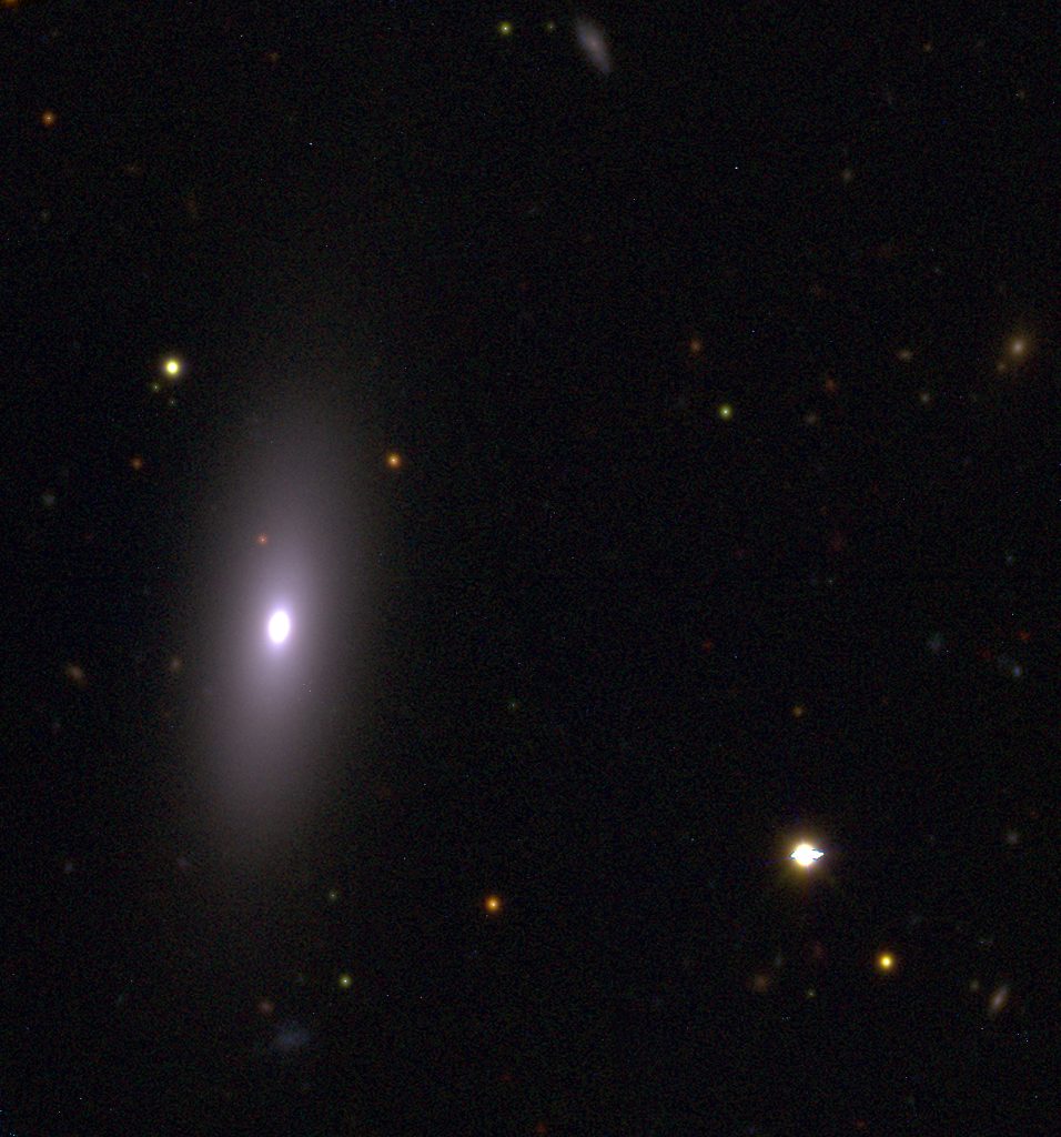
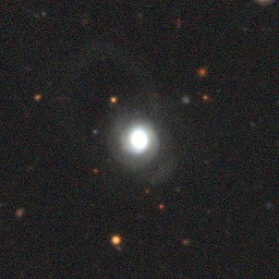
I’ll resume my M31 posts soon (I hope), but I wanted to do a short post on the recent Zoogems HST observation of IC 3025 which is a dwarf elliptical in the Virgo cluster that was selected as part of the “post-starburst” galaxy sample. Thanks mostly to its membership in Virgo this galaxy is fairly well studied and even has multiple HST observations. Just for fun I tried to make a false color RGB image from three observations, with two in the IR through F160W and F110W filters, and the blue channel from the Zoogems observation in F475W.

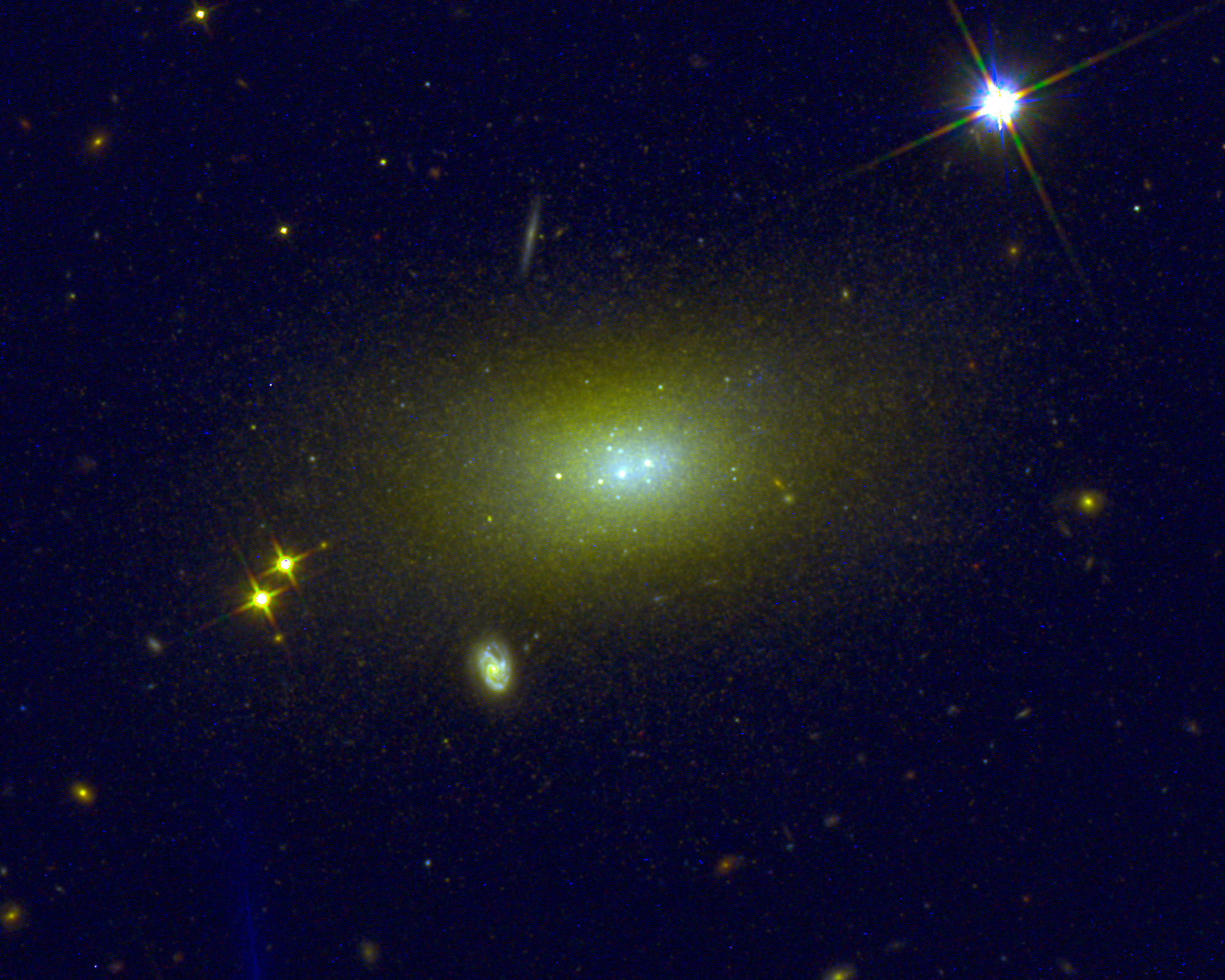
This used a program named SWarp (author Bertin) to rescale and align the images and STIFF (also Bertin) to combine them, with some Photoshop work in a mostly futile attempt to get a more pleasing color balance and clean up some of the hot pixels. I don’t know exactly how STIFF maps counts to gray scale levels, but despite the odd color cast this picture may actually give a reasonably accurate rendering of the relative fluxes in each filter. The galaxy as a whole has a g-J color of about 1.3 mag (based on my measurements with APT and NED) and J-H ≈ 0.2 mag. per Jensen et al. (2015), so an orange or even green color in the body of the galaxy is not so unreasonable.

The blue(er) central region is notable and apparently real also. This is one of a distinct class of dwarf early type galaxies with blue centers, given the designation dE(bc) by Lisker et al. (2006). The blue centers are almost certainly due to recent star formation, as I’ll verify below.

There are 3 bright, unresolved clusters near the center with a number of others scattered around the body of the galaxy. By my measurements with the manual Aperture Photometry Tool the brightest of these has a g band (F475W) magnitude of 20.71 and J (110W) of 20.084, or g-J ≈ 0.62. The other two near the galaxy center are slightly fainter and considerably redder: g = 21.5 and 22.6 for the western and eastern flanking clusters, with g-J ≈ 1.2 for both. Jensen et al. (cited above) measure the distance modulus to be m-M = 31.42, which makes the F475W absolute magnitude of the central cluster equal to -10.71. Like the Zoogems target I discussed several months ago this would be quite luminous for a galactic globular cluster but is typical for a dwarf galaxy’s nuclear star cluster (Neumayer, Seth, and Boker 2020). This distance modulus, which corresponds to a luminosity distance of 19.2 Mpc, is considerably larger than the canonical distance to the Virgo cluster of m-M = 31.09 (per Jensen again). This is one of several lines of evidence that the galaxy is currently falling into the cluster.

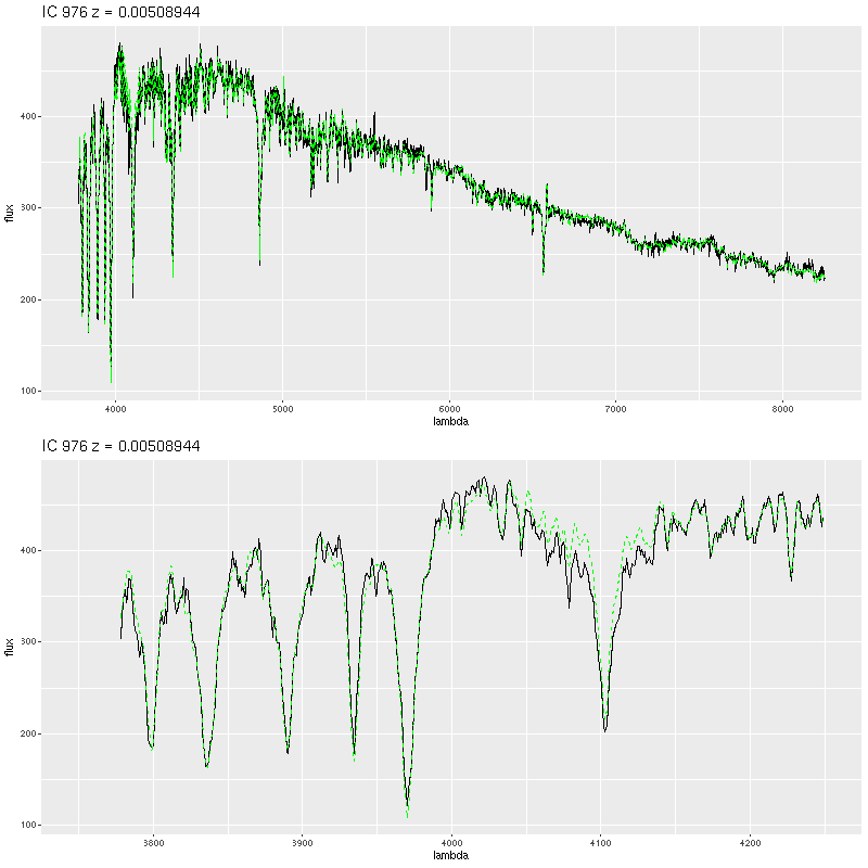
Like the other galaxies in the Zoogems “post-starburst” sample the SDSS spectrum was incorrectly classified by the SDSS spectro pipeline as coming from a star, but this one has a correct redshift and has been used in science studies (for example in Lisker et al. cited above). From the reported position the fiber center was just west of the brightest central cluster and includes both that one and the cluster just to the west. The spectrum is very much typical of a post-starburst, with deep Balmer absorption and a shallow 4000Å break. I measure Hδ_A = 7.24 ± 0.60Å and D_n4000 = 1.26 ± 0.014¹, very similar values to the other two that I posted about last year. Finally, although it’s far from evident on visual inspection, there are firm (4-5 σ) detections of Hα and S[II] 6717, 6730 in emission. No other emission lines were detected.

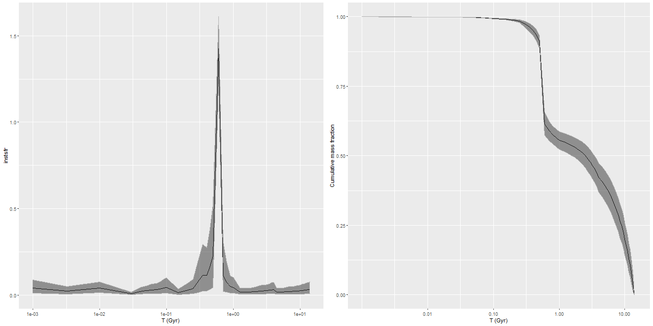
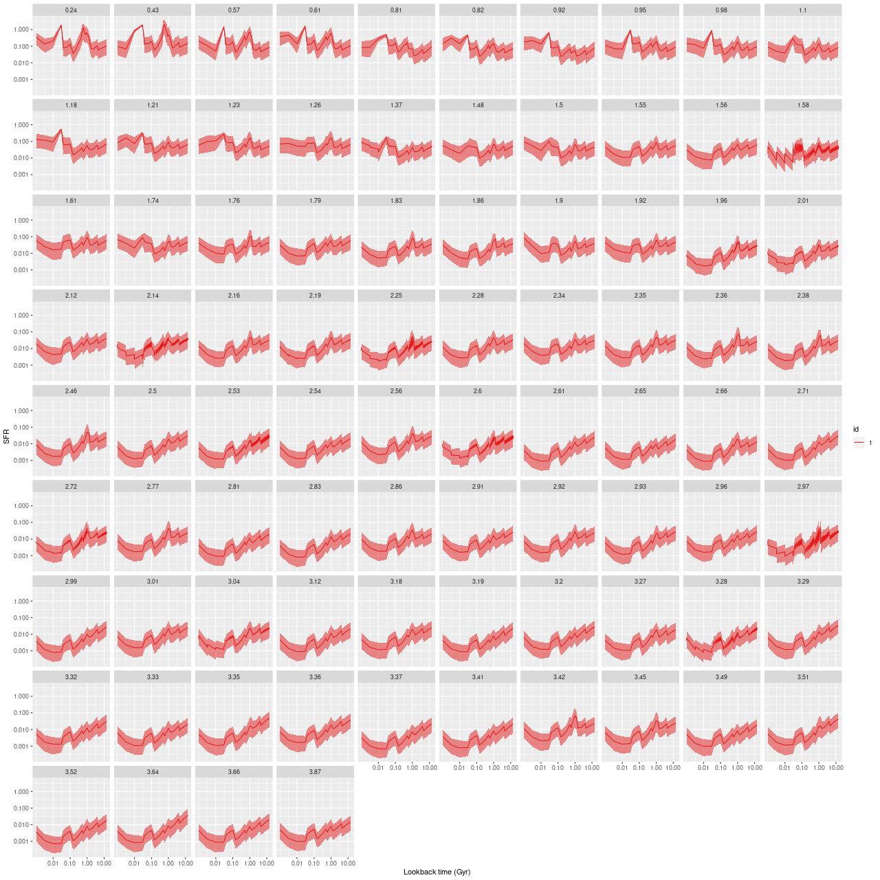
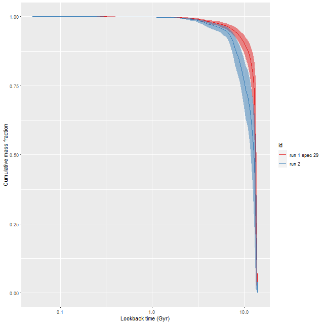
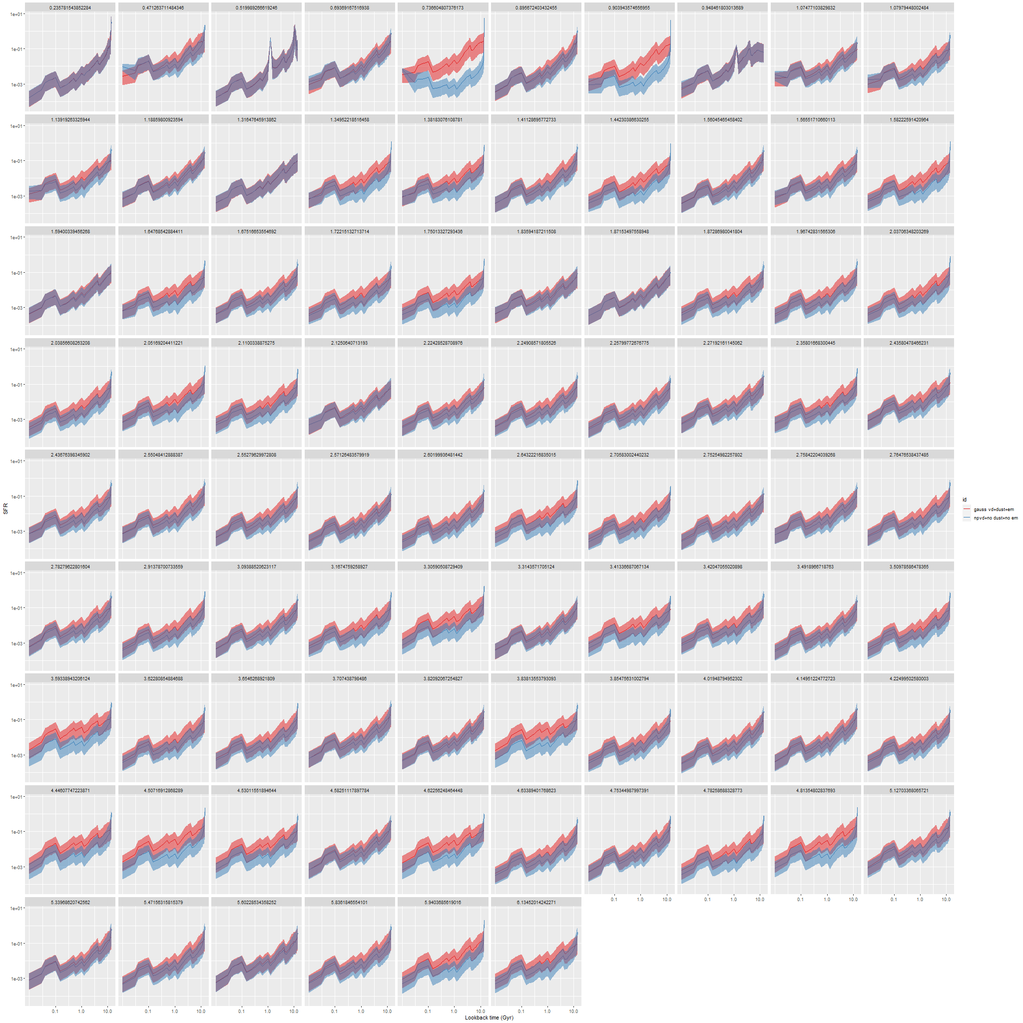
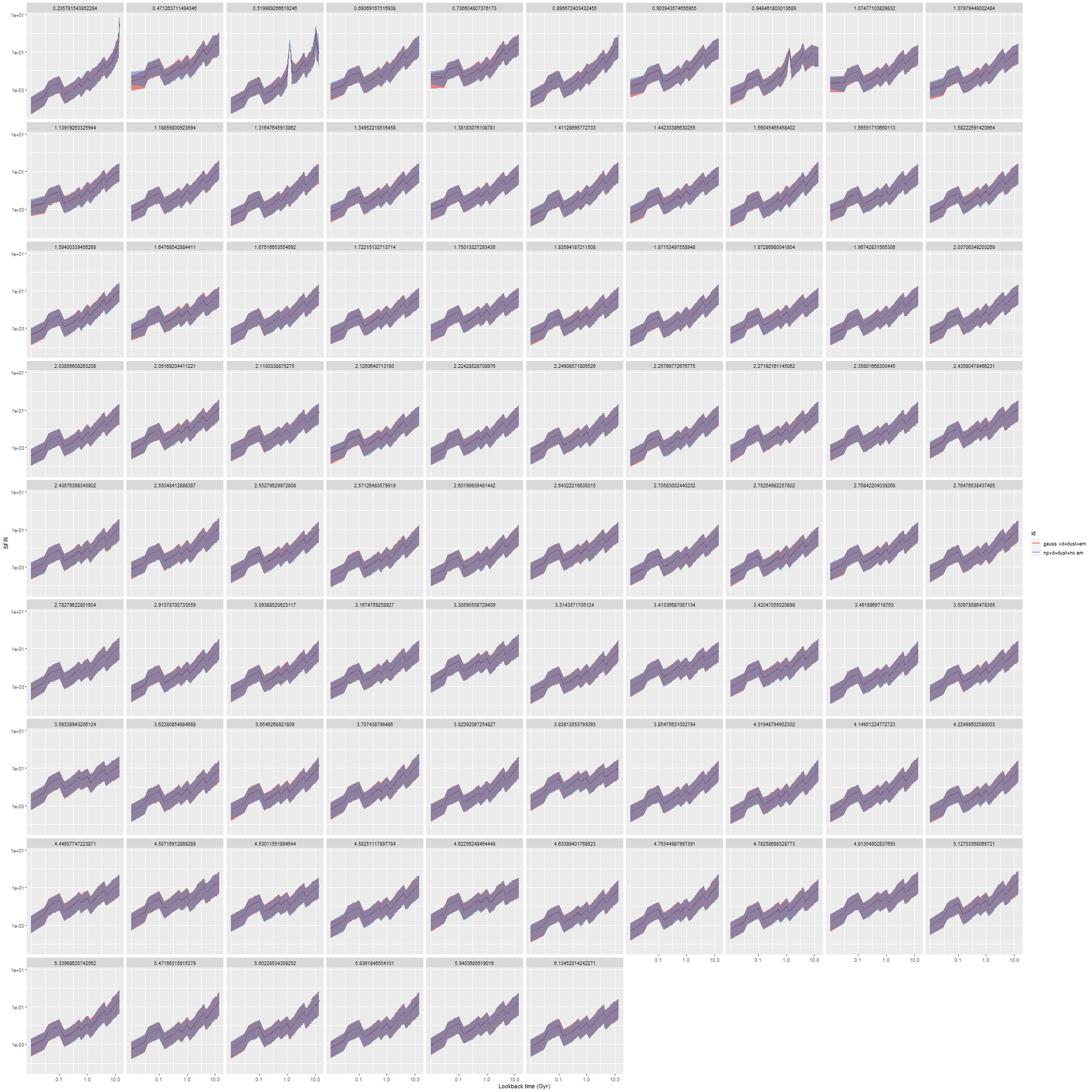
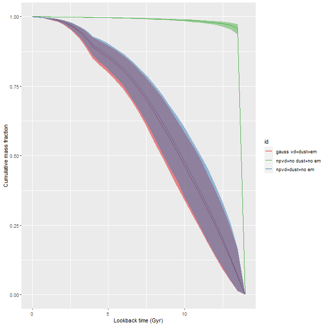
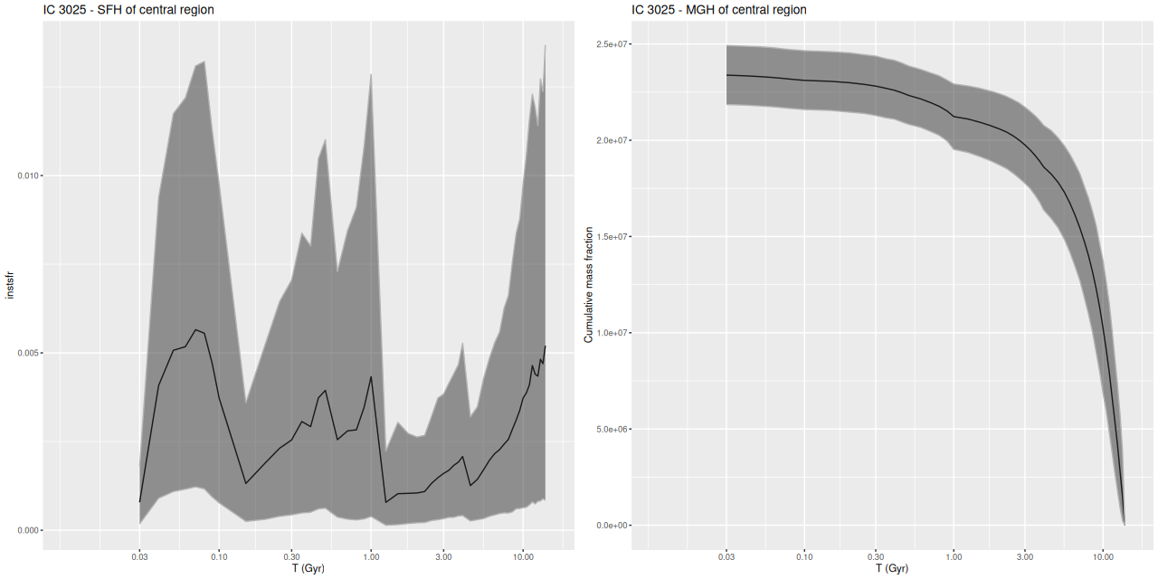
I used my usual star formation history modeling code with the metal poor subset of the EMILES SSP library as described here, which produced the estimated star formation and mass growth histories:

ic3025_sfhmgh — IC 3025 – Star formation history and mass growth history modeled from SDSS spectrum

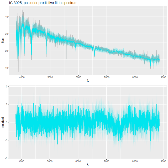
with a very good fit to the data except for a small region around 7500Å (which is often the case with the EMILES library):

ic3025_ppfit — IC 3025 – posterior predictive fit to spectrum from SFH model

My results can be compared fairly directly to an analysis by Lisker et al. (cited above), who performed some simple stellar population modeling on SDSS spectra with what appears to be their own unreleased code. They limited their populations to 3 discrete ages with the oldest fixed at 5 Gyr and the mass fractions and ages for the other 2 chosen from a finite set of possible values.

Perhaps surprisingly my results agree rather well with theirs. For VCC 21 (the Virgo Cluster Catalog designation for IC 3025) their best fit had about 9% of the total mass in young and intermediate age populations, with the young population chosen at 9 Myr age and 0.3% of mass and the intermediate population age of 509 Myr.

My models also show three broad periods of star formation with some lulls in between that can conveniently be divided into young, intermediate, and old populations. The youngest SSP models in my metal poor subset are 30 Myr, so of course there can’t be any truly young populations in the model. The peak in recent star formation was at ~70 Myr with a steep decline at the youngest lookback times. Around 1% of the present day stellar mass in the fiber footprint is in stars younger than 100 Myr, with just under 10% under 1 Gyr.

Based on the colors we can infer that the acceleration of star formation that began ~1 Gyr ago was limited to the central region and the presumed nuclear star cluster. The remainder of the galaxy and its cluster system must already have been quiescent by then.

Edit

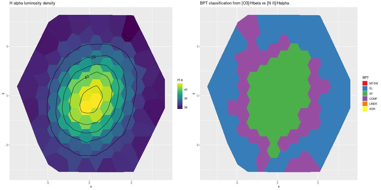
I mentioned above my SFH models indicated there were firm detections of Hα and the [S II] doublet in emission. Although [N II] wasn’t detected at better than the 1σ level it’s still possible to make a strong line metallicity estimate from the posteriors. I also plot the marginal posterior for Hα luminosity below:

ic3025_ha_oh — IC 3025 (L) Hα luminosity from SDSS spectrum (R) log(O/H) estimated from [N II]/Hα and [S II]/Hα

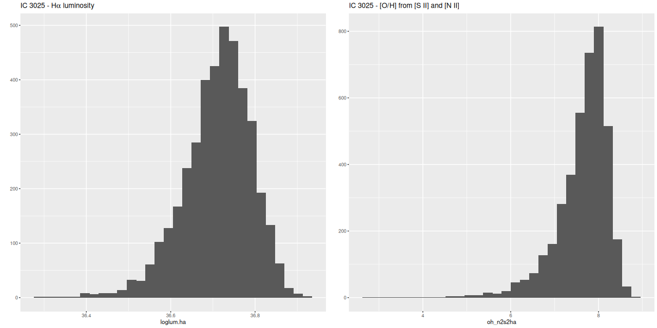
Using Calzetti’s calibration of the Hα – SFR relation this implies a current day star formation rate ~10^-4.5 M_☉/yr. This should be considered an upper limit since we don’t know the ionizing source. Using Dopita’s calibration of the [N II]/Hα plus [S II]/Hα strong line metallicity estimator the upper limit to 12+log(O/H) is around 8, which is subsolar by almost an order of magnitude.

2022-09-17

IC 976

I’m going to try to keep this one short. IC 976 is another post-starburst galaxy that was selected and recently observed by HST for the Zoogems project (proposal ID 15445, PI Keel). I took a shot at creating a color image by combining the ACS observation taken with the F475W filter (approximately equivalent to SDSS g band) with r and z band images from the Legacy Survey. Well that wasn’t too rewarding since this galaxy appears quite featureless.

Like the galaxy in the previous post the SDSS spectro pipeline misclassified this galaxy’s spectrum as a star with a recession velocity of ≈ 1200 km/sec. Unlike the galaxy in the previous post IC 976 is well known to have a post-starburst nuclear spectrum, and its correct heliocentric redshift of 0.00509 is listed in NED and confirmed with my own redshift estimation code. If that’s its Hubble flow redshift (doubtful) its distance would be about 21.8 Mpc (distance modulus m-M=31.7) and the 3″ SDSS fiber would cover 315 pc.

IC 976 redshift measurement — SDSS spectrum of IC 976 nucleus with best fit template overlay

Once again I ran my SFH modeling code on the SDSS spectrum, using only my metal rich PYPOPSTAR+EMILES ssp library, with results below:

Modeled star formation and mass growth histories of central region of IC 976 from SDSS spectrum 340044889930622976.

Despite the superficially similar spectra¹ this model favors an older (peak at 800 Myr lookback time), stronger, and shorter burst than the previous example. The model’s burst strength of ≈ 40 % of the present day stellar mass seems high, but the estimated total stellar mass within the fiber footprint is only ≈10^8.5 M_☉, which is likely a small fraction of the galaxy’s total stellar mass. For a rough estimate of the total mass the SDSS g band Petrosian magnitude is listed as 13.6, making the absolute magnitude -18.1. With a solar g band absolute magnitude of 5.11 the galaxy’s luminosity is ≈ 10^9.3 L_☉, and assuming a stellar mass to luminosity ratio around 1 the mass would therefore be ≈ 2×10⁹ M_☉. If the merger added a little over 10⁸ M☉ to the system as implied by this model the mass ratio of the progenitors would be on the order of 20:1.

IC 976 was one of 7 post-starburst galaxies in an IFU based spectroscopic study by Pracy et al. (2012). This galaxy² had a very strong negative radial gradient in the Balmer absorption index, as did 5 of the 6 others in the study. They concluded that centrally concentrated starbursts fueled by minor mergers was the most likely cause of their present evolutionary state. The lack of any apparent tidal features in the available imaging of this galaxy likely reflects the age of the merger and mass ratio of the progenitors.

2022-07-162022-08-18

Journal notes: Haines et al. (2015), “Testing the modern merger hypothesis…”

While browsing through the ADS listing of papers that cite Schawinski’s paper that I’ve been discussing for a while I came across this one by Haines et al. with the full title “Testing the modern merger hypothesis via the assembly of massive blue elliptical galaxies in the local Universe”. Besides being on the same theme of searching for post-starburst or “transitional” galaxies in the local universe that I’ve been pursuing for some time the paper was interesting because it made use of IFU based spectroscopic data that predates MaNGA. As it happens 4 of the 12 galaxies have observations in the final MaNGA release, providing an excellent opportunity to compare results from completely independent data sets.

The “modern merger hypothesis” that the authors tested relates to a topic I’ve discussed before, which is that N-body simulations show that strong, centrally concentrated starbursts are a possible outcome of major gas rich galaxy mergers around the time of coalescence. If some feedback process (an AGN or supernovae) rapidly quenches star formation there will ensue a period of time when the galaxy will be recognizable as post-starburst.

In a series of long and rather difficult (and influential judging by the number of citations) Hopkins and collaborators (2006, 2008a, 2008b) have made a case that major gas rich mergers with accompanying starbursts are in fact the major pathway to the formation of modern elliptical galaxies. They claim that their merger hypothesis accounts for a variety of phenomena, including the growth and evolution of supermassive black holes and quasars.

The specific aspect of the merger hypothesis this study tried to address was the prevalence of strong centrally concentrated starbursts in a sample of ellipticals in the process of forming as evidenced by visible disturbances consistent with recent mergers. The main tool they used was a suite of simple star formation history models with exponentially decaying star formation rate with single (also exponentially decaying) bursts on top of varying ages and decay time scales. They used these to predict just two quantities: Balmer absorption line strength measured by the average of the Lick Hδ_A and Hγ_A indexes, and the 4000Å break strength index D_n4000. For reference here is a screen grab of their model trajectories:

Predected trajectories in the Hδ – D_n4000 plane per Haines et al. (2015). Clipped from the electronic journal paper.

This is a pretty standard calculation variations of which have been performed for decades, and this graph looks much like others I have seen in the literature. A fairly basic problem with it though is that position in the Balmer – D4000 plane doesn’t uniquely constrain even the recent stellar evolution. In astronomers’ parlance there is a “degeneracy”¹ between burst strength (if any) and burst age. This is a well known problem with the Balmer line strength index that was already recognized by Worthey and Ottaviani (1997), who developed these indexes. Adding a second index in the form of the 4000Å break strength doesn’t break the degeneracy: there are regions of the plane where bursting and non-bursting populations overlap, as can be seen clearly in the graphic above. This is actually a problem for any attempt to identify post-starburst galaxies. After correcting for emission most ordinary starforming galaxies have strong Balmer absorption lines, so using that index alone will certainly produce many false positives. On the other hand selection criteria like those used by Goto and many others before and after — selecting for both strong Balmer absorption and weak emission — will capture only a small interval in post-starburst galaxies’ life cycles.

hd_d4000_bigsample — Hδ line strength vs. 4000Å break index for a large (~380K) sample of SDSS galaxy spectra. Measurements from the MPA-JHU analysis pipeline downloaded from SDSS Skyserver

Let’s get to results. Some basic details of the sample are in the table below. Morphological classifications are from McIntosh et al. (2014) as given in this paper. The abbreviations are SPM: spherical post merger; pE: peculiar Elliptical. The two marked pE/SPM didn’t have a strong consensus among several professional classifiers. I list them in order of my own visual impression of degree of disturbance. I also list redshifts taken from the MaNGA catalog and Petrosian colors.

NED name	NYU ID	mangaid	plateifu	Morph	z	u-r	g-i
NGC 3921	541044	1-617445	10510-6103	SPM	0.019	1.97	0.86
MRK 385	719486	1-604970	8940-6102	pE/SPM	0.028	1.43	0.63
MRK 366	100917	1-603309	7993-1902	pE/SPM	0.027	1.59	0.79
NGC 1149	22318	1-37155	8154-6103	pE	0.029	2.29	1.11

Columns: (1) Common catalog designation (NED name). (2) NYU VAC ID. (3) MaNGA mangaid. (4) MaNGA plateifu. (5) Morphology (see text). (6) redshift from MaNGA DRP catalog. (7-8) Petrosian u-r and g-i colors from NYU VAC via the MaNGA DRP catalog.

The main prediction of the merger with accompanying centrally concentrated starburst hypothesis the paper tests is that the Balmer absorption index should be large and have a negative gradient with radius while the 4000Å break strength should be low with a positive gradient. The authors concluded that only one member of their sample — nyu541044 — clearly falls in the post-starburst region (marked as region 4 in the graph above) of the <Hδ, Hγ> – D_n4000 plane. The two pE/PM galaxies, both of which are in my sample, lie in the starforming region 1. They inferred from this that these galaxies are undergoing at most a weak burst. I’m going to mildly disagree with that conclusion.

Screenshot from 2022-07-07 15-23-36 — Measured values for the specified indexes from Haines et al. (2015). Clipped from the electronic journal paper.

I have calculated the pseudo Lick index Hδ_A and D_n4000 as part of my analysis “pipeline” since I started this hobby. I actually make these measurements in the initial maximum likelihood fitting step since they don’t depend on modeling except for small (usually) emission corrections. I don’t calculate an Hγ index, but its theoretical behavior is similar to Hδ. I’m trying here just to verify the approximate magnitude and radial trends of the chosen indexes. The two IFUs used in the Haines study had larger spatial coverage than these MaNGA observations (but much smaller wavelength coverage, which will become important). Instead of their strategy of binning in annuli I used my usual Voronoi binning strategy with a minimum target S/N. There were some oddities in the NYU estimates of effective radii so I chose to use distances from the IFU center in kpc for these plots. The distances assigned to the multiply binned spectra are the same as Cappelari’s published code produces; for single fiber spectra it’s just the position of the fiber center.

My measurements agree reasonably well with those of Haines et al. All three of the most disturbed galaxies have central Hδ indexes > 5Å with NGC 3921 (plateifu 10510-6103, nyu541044) having a larger central value and steeper gradient in the inner few kpc than the two pE/SPM galaxies. The fourth galaxy shows no obvious trend in either index with radius². The central values where the S/N is highest are in good agreement.

Lets turn to the results of star formation history models, which I ran on all 4 data sets. First, here are 100Myr averaged star formation rate density and specific star formation rate versus distance:

Star formation rate density vs. distance from IFU center (kpc) for 4 disturbed early type galaxies.

Specific star formation rate density vs. distance from IFU center (kpc) for 4 disturbed early type galaxies.

Three of these galaxies are clearly experiencing centrally concentrated episodes of star formation, and two are at or near starburst levels in specific star formation rate near their centers. As seen below two of these straddle my estimate of the “spatially resolved star forming main sequence” while the one presumed post-starburst galaxy reaches it in the central region.

mstar_sfr_4spm — Star formation rate density versus stellar mass density for 4 disturbed early type galaxies

As I’ve shown several times before there’s a reasonably tight linear relationship between modeled star formation rate and Hα luminosity density. The plot shows Hα luminosity density corrected for modeled stellar redenning, which certainly underestimates attenuation in emission regions. The modeled star formation rates are consistently above the Kennicut relation shown as the straight line as I’ve seen in every sample I’ve looked at.

Star formation rate density vs. Hα luminosity density for 4 disturbed early type galaxies

Finally, lets take a look at detailed star formation histories. Instead of my usual practice of plotting them all in a grid here I just display 2 binned star formation histories. One comprises the innermost 7 bins, which since the fibers are arranged in a hexagonal grid should form a regular hexagon around the IFU center. These range in “radius” from about 0.75 to 1.1 kpc in these four galaxies. The second is for an “annulus” in approximately the outer kpc of each IFU. The extent of the IFU footprints ranges from 3.1 to 5.9 kpc. I calculate these by summing the contributions in each SFH model contributing to the bins, not by running new models for binned spectra. Since the dithered fiber positions overlaps this overestimates the total mass in each bin, but I care about the shape and timing of events rather than the absolute values of star formation rate estimates.

The next 4 plots display the results. Lookback time is logarithmically scaled with the same range and ticks for each SFH. Vertical scales are linear and differ for each graph. The graphs are in the same order as the basic information table above. As I’ve written before these models “want” to have smoothly varying mass per time bin which has the unfortunate effect of producing jumps in the apparent SFR when the bin widths change. In the BaSTI isochrone based SSP models these occur at 100 Myr, 1 Gyr, and 4 Gyr and can sometimes be quite prominent.

With caveats out of the way the one clear post-starburst in the sample had (per the model) a powerful and short starburst at ≈300 Myr lookback time, with a small amount continuing to the present (this can’t be seen at the scale of the graph, but ongoing star formation is ~1 M_☉/yr). The total mass contribution from the burst and subsequent star formation is around 15%.

The two apparent ongoing starbursts have later bursts of star formation that are slightly weaker in terms of total mass contribution and peak star formation rate, but still quite significant. All three of the starburst/post-starburst galaxies appear to have had two major waves of late time (last ~2 Gyr or less) star formation. As I’ve written before in merger simulations the progenitors usually complete a few orbits before coalescence, with some enhanced star formation around each perigalactic passage. I hesitate to take these models that literally.

Turning finally to the last and least disturbed galaxy, NGC 1149, despite the bursty appearance of the SFH there’s no evidence for a major starburst in the cosmologically recent past. Whether an older starburst can be detected in this kind of modeling approach needs investigating.

One last set of graphs that may be useful. These show cumulative star formation histories — basically the cumulative sum of mass contributions starting from the oldest time bin. This is similar to a mass growth history which is a popular visualization. In my calculation of the latter the contributions are to the present day stellar mass, so an allowance for mass loss and remnant mass is made³. The graphs are for the central regions only. Note the major virtue of these is that the contributions of major episodes of star formation can be estimated at a glance.

Cumulative star formation histories for central regions of 4 disturbed early type galaxies

To wrap up this part of the post 3 of these galaxies are compatible with the “modern merger hypothesis,” that is they have experienced centrally concentrated but spatially wide spread starbursts. The reason two of them don’t have post-starburst characteristics in the Hδ – D4000 plane is their starbursts are still underway. The current burst of star formation contributes about 5-10% of the mass in the central regions of these two. How much more is available is unknown (at least to me until I get around to finding out if there are HI mass estimates available).

Future plans: I’ve completed model runs on the 24 “post-starburst” galaxies in the MaNGA ancillary program dedicated to them. I may have something to say about them. I also may have something to say about one of the Zoogems targets that I had a small part in selecting.

2022-06-21

A little more on Schawinski’s blue early type galaxies

As I mentioned two posts ago there are 24 of these galaxies in the final MaNGA data release, a remarkable 11% of the full sample. I ran my SFH model code on all of these along with the prerequisite redshift offset routine¹. SDSS thumbnails of the sample are shown below. As expected none of these have significant spiral structure visible at SDSS resolution, but at least a few are noticeably disturbed.

thumbnails_blueetg — SDSS thumbnail images of Schawinski et al.’s blue early type galaxies in MaNGA final data release (SDSS DR17)

I’m just going to discuss a few topics in this post. I’ll save a more detailed discussion for when I’ve completed analysis of the ancillary post-starburst sample, which is underway now. First, here are velocity fields calculated for the stacked RSS data, with a signal to noise cutoff of 3, the same as I used for my analysis of rotation curves of disk galaxies. Note in the graphic below the ordering is different from the image thumbnails.

vfs_blueetg — Line of sight velocity fields of Schawinski et al.’s blue early type galaxies in the final MaNGA data release

By my count (based entirely on visual inspection) all but 2 of these exhibit large scale rotation, with perhaps 15 or 16 classifiable as regular rotators with the remainder containing multiple velocity components including a couple with (perhaps) kinematically distinct cores. The preponderance of rotating systems surprised me at first, but according to a review by Cappellari (2016) large scale rotation is predominant at least at lower stellar masses (Schawinski et al. characterized their sample as being “low to intermediate mass” among early type galaxies). The velocity fields indicate that many of these contain stellar disks, perhaps embedded in large bulges. That’s still consistent with classification as “early type galaxies.” Apparently the original Galaxy Zoo classification page used the term “elliptical” as the early type galaxy choice, but in the data release paper by Lintott et al. (2011) there’s a statement that the “elliptical” class should comprise ellipticals, S0’s, and perhaps Sa’s from Hubble’s classification scheme.

Depending on how my effort to do non-parametric line of sight velocity modeling goes I may return to examine the kinematics of this sample in more detail, in particular to look for evidence of gas and stellar kinematic decoupling.

Turning to the recent star formation history this sample runs the gamut from large scale starbursts to passively evolving as seen in the plot of (100 Myr averaged) star formation rate versus stellar mass density for all analyzed binned spectra (of which there were 1525 in the full sample). For reference the straight line is my estimate of the center of the local “spatially resolved star formation main sequence.” This is just a weighted least squares fit to the sample of 20 non-barred spirals with star forming BPT diagnostics that I discussed some time ago. My SFMS relation has the same slope as estimated by Bluck but is offset higher by about 0.7 dex, which probably just reflects the very different methods used to estimate star formation rates. The contour lines are the densest part of the relationship from the passively evolving Coma cluster sample that I also discussed in that post. The majority of the blue etg sample falls in the green valley, consistent with Schawinski et al.’s observation that only about 1/2 of the sample showed evidence for ongoing star formation.

sfr_mstar_blueetg — “Spatially resolved” star formation rate density versus stellar mass density for 24 blue early type galaxies in final MaNGA data release. Contour lines are corresponding values for 33 passively evolving Coma cluster galaxies.

Most of the points offset the most on the high side of the SFMS come from just two galaxies: MRK 888, which I’ve discussed in the last few posts, and SDSS J014143.18+134032.8 (this is apparently not in any “classical” catalog). The legacy survey cutout below clearly shows an extended tidal tail that’s a certain sign of a relatively recent merger.

SDSS J014143.18+134032.8, a disturbed, star-bursting blue early type galaxy

I just want to take a quick look at this one: below are maps of the star formation rate density and SSFR as well as scatterplots of the same against distance from the IFU center. As with MRK 888 ongoing star formation is widespread with a peak near the center, a classic case of a merger fueled starburst. In this galaxy star formation peaks in a ring somewhat outside the nucleus. The ring can be seen clearly in the SDSS cutout and must consist of HII regions.

8095-1902_sfr_ssfr — SDSS J014143.18+134032.8 (mangaid 1-41541; plateifu 8095-1902) Star formation rate density and specific star formation rate – maps and scatterplots against radius in kpc.

Schawinski et al. briefly discuss the possibility that their blue ETG’s could be progenitors of E+A (aka K+A) galaxies. This galaxy and MRK 888 are plausible candidates — if star formation shut off rapidly they would certainly exhibit strong Balmer absorption for a time after emission lines disappeared since they already do. Other members of this sample are already fading towards the red sequence, and if they ever qualified as “post-starburst” it must have been in the past.

I plan to look at star formation histories in more detail after I’ve completed model runs on the MaNGA post-starburst sample.

2022-01-282022-04-02

What fraction of Schawinski’s “Blue early type galaxies” are ellipticals?

The first iteration of Galaxy Zoo led to several collections of distinct objects, including a sample of 215 “blue early type galaxies” published in Schawinski et al. (2009)¹I found this an interesting group of galaxies, partly because of a possible link to post-starburst (K+A) galaxies that was discussed in the original paper. The authors discuss at some length the likelihood that these are results of mergers in the cosmologically recent past, with at least one of the progenitors being gas rich. Many (at least 25% and possibly more than half) were found to be currently starforming and the rest likely to have only recently ceased forming stars as inferred from their blue colors.

The ongoing Zoogems program has 12 of Schawinski’s blue ETGs on its target list, of which 6 have been observed so far as of mid-January 2022. Somewhat surprisingly there are 24 in the final MaNGA release, over 11% of the sample!

Taking a look at the 6 with HST observations I would say none of these are typical ellipticals. Five show some degree of spiral structure although in 4 it’s embedded in a more diffuse body. One appears to me to be an S0 with both inner and outer rings — this is in agreement with the one published morphological classification I’ve found. All of the others appear more disky than ellipsoidal to me, although this is just my possibly flawed qualitative judgment. At least two are visibly disturbed. One (CGCG 315-014) is connected to a nearby galaxy with a long tidal tail as seen in the Legacy Survey thumbnail below. Markarian 888, which will be the subject of the rest of this post, has shells that extend well past the main body of the galaxy and prominent, centrally concentrated dust lanes.

So far it’s the only Zoogems blue etg target with a MaNGA observation (two others on the target list are in MaNGA but of course there’s no guarantee they will ever be observed). As is often the case the IFU could have been larger — this was observed with a 37 fiber bundle giving 111 dithered spectra in the RSS file.

MRK 888 SDSS thumbnail with MaNGA IFU footprint

As always the first step in analyzing these data is to estimate redshift offsets for each spectrum, and from there we get a velocity field, which in this case shows a rapid rotator with a fairly symmetrical radial velocity pattern.

Mrk 888 (MaNGA plateifu 9894-3703) velocity field

Visual inspection suggests the line of sight velocity distribution is consistent with a rotating thin disk, so I fed the data to my Gaussian process based rotation modeling code, with results summarized below. In fact the model does an excellent job of accounting for the data, with residuals (not shown) from the model fit (top right) in a range of ±15 km/sec. One unusual feature of the velocity field is the rotation velocity turns over at somewhat less than one effective radius. Whether the rotation curve declines smoothly outside the IFU footprint or is kinematically disconnected from the outer parts of the galaxy is of course unknowable at this time.

I also ran my usual star formation history modeling code on the data binned to 97 spectra. First, here are some summary results. The stellar mass density declines roughly exponentially, which is consistent with a disky morphology:

Model estimate of stellar mass density vs. radius

Next are maps of the estimated Hα luminosity density and, on the right, the BPT classification from the [O III]/Hβ vs. [N II]/Hα diagnostic. The contours are elliptical with major axes closely aligned to the rotation axis (the posterior mean for the angle is the dashed line in the velocity field plot above). Again, the emission appears to arise in a disk.

The proper interpretation of the “composite” BPT classification is something I think I’ve written about in the past. It was originally suggested to indicate a mix of AGN and stellar ionization, but here it arises in a thin ring of weak but detectable emission just outside the star forming region. If it’s truly composite it’s likely to arise from a mix of weak star formation and ionization by hot evolved stars. In any case there’s no evidence for an AGN in the optical data.

(L) Hα luminosity density (R) BPT classification from [O III]/Hβ vs {N II]/Hα diagnostic

Next are maps of the modeled (100 Myr average) star formation rate density and specific star formation rate, and in the second row scatter plots of the same estimates against radius in kpc. The trends with radius are somewhat unusual, especially for SSFR which in a normal disk galaxy typically increases with radius even if the highest total star formation rates are centrally concentrated. Highly centrally concentrated star formation in the aftermath of mergers is predicted by some simulations.

(TL) star formation rate density; (TR) specific star formation rate; (bottom row) scatter plots vs. radius

A couple more graphs will round out my discussion of summary model estimates. As I’ve shown several times before there’s a pretty tight linear relationship between modeled SFR density and estimated Hα luminosity density. In this plot Hα is corrected for modeled stellar attenuation, which is expected always to underestimate the attenuation in emission line emitting regions. That, and the fact that Hα emission and the model star formation rate estimates probe order of magnitude different time scales probably account for the systematic offset from the standard calibration given by the straight line.

Model star formation rate density vs. Hα luminosity density corrected for *stellar attenuation*. Straight line is calibration from Calzetti (2012).

And, once again I show a map of the modeled optical depth of stellar attenuation. The region of highest optical depth nicely tracks the visible dust (the HST image at the top is rotated about 90º from the SDSS image). Outside the dusty region there appears to be a shallow gradient, which might indicate that the nearer side is to the northeast.

Map of modeled optical depth of stellar attenuation

Finally here are plots of the model star formation history for all spectra ordered by distance from the IFU center. In the inner 1.5 kpc or so there’s some recent burstiness with possibly a very recent acceleration of star formation. For reasons I’ve discussed recently I don’t take either the timing or magnitude of bursts of star formation too seriously, but the behavior of the models is consistent with a recent revival of star formation due presumably to a merger, for which there are multiple lines of evidence.

model star fomation histories for all spectra

With 24 of these galaxies and another 31 from the compilation of Melnick and dePropris and the post-starburst ancillary program in the final release of MaNGA these samples satisfy my criteria of being manageably sized for my computing resources while large enough to say something about the groups. So, when time permits I plan to take a look. I already have the data in hand.

2022-01-152022-01-17

NGC 810 – interesting kinematics in a Zoogems and MaNGA target

The final release of SDSS MaNGA went public back in early December as promised, and I’ve spent the last month or so of my hobby time looking for manageable sized samples of interesting galaxies. One sample I looked at out of curiosity was the Zoogems target list, which is an HST gap filler imaging program with about 300 galaxies selected (mostly) by Galaxy Zoo volunteers. It turns out there are 11 targets with MaNGA data, of which 5 have been observed by HST so far.

As can be seen from the thumbnails above this is a pretty diverse lot, with several in progress mergers and merger remnants, some normal looking spirals at least two of which were from Masters’ red spirals sample, and 3 of Schawinski’s blue early type galaxies. Only one of those 3 has HST imaging so far (number 8 in the thumbnails above), although there are a surprising 24 blue ellipticals in the final MaNGA release out of 215 in Schawinski’s original sample.

Of the 5 Zoogems galaxies that have been observed so far the one that caught my eye as deserving an early look was number 3 in the top row, NGC 810, an apparent elliptical with an unusual dust lane that’s almost perfectly aligned with the minor axis. There are also hints of shells indicating a likely merger sometime in the past.

NGC 810 HST ACS, proposal id 15445, PI Keel

The MaNGA data, which is new in DR17, only covers the central part of the galaxy with the companion just photobombing the edge. A larger IFU would have been nice for this observation, but the data quality is better than average in terms of nominal signal to noise. I was able to use all 183 fiber/position combinations in the RSS file without binning.

NGC 810 – plateifu 9514-6101 – MaNGA IFU footprint

The first step in the analysis process after loading the data is to estimate redshift offsets from the system redshift for each spectrum, and from that it’s straightforward to calculate a velocity field, which in this galaxy looks like¹:

NGC 810 (plateifu 9514-6101) – losvd estimated from cube

It turns out the redshift assigned to this system was that of the companion galaxy, which was the only SDSS spectroscopic target in the immediate vicinity and is evidently blueshifted by ~350 km/sec from the target. What’s more interesting though² is the apparent rapidly rotating disk that’s aligned with and somewhat thicker than the dust lane. There may also be overall prolate rotation outside the disk although the presence of the companion makes it hard to tell based solely on visual inspection. In hopes of separating out multiple velocity components I returned to the non-parametric line of sight velocity distribution models that I wrote some posts about last year. Unlike the ones I practiced on previously this galaxy has non-negligible amounts of emission, at least in the central region, so I just temporarily masked the regions around the emission lines that I fit. That results in a pure stellar velocity distribution. The results were a bit surprising:

NGC 810 (plateifu 9514-6101) (L) velocity field estimated from RSS file (M) stellar velocity offsets (R) net stellar velocity

In the left pane above is the velocity field from the RSS data, with the system redshift adjusted to the IFU center. For the LOSVD models I set the adopted redshift of each spectrum to the system redshift plus the offset calculated previously. Now I had hoped to be able to cleanly separate the contribution of the companion from that of the main galaxy, which so far I haven’t been able to do. But what I did find that was unexpected is that the average stellar velocities in the disk partially offset the original measurements (middle pane), so the net stellar velocity field shows a much more slowly rotating stellar disk.

As I’ve written before I use a set of 15 eigenspectra from a principal components analysis of some tens of thousands of SDSS spectra that I performed some years ago for redshift offset estimation. Those galaxies were of all types and include systems both with and without significant emission. The redshift estimation routine just does straightforward template matching and returns a single value for the best fitting offset. Since the templates encode information about both emission and absorption lines that estimate could be most applicable to the ionized gas, stars, or some combination. In this case it’s possible emission lines were driving the original fits, implying the gas and stars in the disk are kinematically decoupled. I have not verified that though.

Another issue I noticed is that the stellar velocity field from the official MaNGA Data Analysis Pipeline looks rather different from mine, with barely a hint of a kinematically distinct disk. This wasn’t really evident in the Marvin webpage, which makes some really unfortunate choices for color palettes. So here is the same data rendered with a more nearly perceptually uniform rainbow palette³:

NGC 810 (plateifu 9514-6101) Stellar velocity field per MaNGA DAP

I decided to re-run my LOSVD modeling code on the RSS data, this time setting the redshift offset to 0 for each fiber, so this is now measuring velocities relative to the overall system velocity. I also used a larger convolution kernel (25 vs. 21 in the first set of runs). The map of the average velocity offsets is:

NGC 810 (plateifu 9514-6101) Stellar losvd from nonparametric model

Although not a perfect match this is somewhat closer to the DAP map. I suspect what’s happening here is that there really are at least two, and more likely 3 distinct kinematic components. I haven’t read the DAP release paper in a while and don’t know exactly how they estimate stellar velocities, but in any case their model just returns a single value for visualization purposes. To see the (possible) complexity of the actual data here are the results for a single fiber with the largest positive velocity offset in the map above. Again, I don’t know how much of the structure in the posterior distribution of the convolution kernel is real, but it’s evident there’s more complexity than is captured in the first two moments shown in the middle and right panes.

Besides the kinematic modeling I did run star formation history models on the full RSS data set using the same tools as in recent posts. I’m not going to discuss them in detail, but some summary maps are worth showing. In the graphic below these are, from top left, stellar mass density, Hα luminosity density uncorrected for attenuation, SFR density (as usual 100Myr average), and stellar dust attenuation.

There’s no sign of a disk in the stellar mass map, which faithfully follows the distribution of light. A disk is visible in Hα and the small amount of recent starformation is also confined to a disk and nuclear region. In the fourth pane I show the modeled stellar dust attenuation, mostly just to demonstrate that this component of the model does capture something of reality.

ngc810_model_summaries — NGC 810 – a sampling of quantities derived from star formation history models

Getting back briefly to the first paragraph, there are 8 post-starburst galaxies from the catalog of Melnick and de Propris and 24 from an ancillary program to observe post-starburst galaxies from various sources that was added for DR17. There’s just one galaxy from the former catalog in the latter set, so that makes 31 total, an easily manageable number. There are also 24 of Schawinski’s blue ellipticals. Of course there are many disk galaxies, far too many for me to look at.

2021-07-142021-07-14

Do the details of the line of sight velocity distribution matter for star formation history modeling? Probably not much.

I decided to try a set of models for one galaxy – NGC 4889 (with MaNGA plateifu 8479-12701), which had the highest overall velocity dispersion of the Coma sample I’ve been discussing in the last several posts. It also has some evidence for multiple kinematic components which isn’t too much of a surprise since it’s one of the central cD galaxies in Coma. The SSP model spectra fed to the SFH models were preconvolved with the element wise means of the LOSVD convolution kernels from the velocity distribution modeling exercise. Again, this is an expedient to avoid what could otherwise be prohibitively computationally expensive. The models I ran were the same as described back in this post — these ignore emission but do model dust attenuation with the usual modified Calzetti attenuation relation.

To get quickly to the results, here are model star formation histories compared to the previous runs that used the full model in its current form. Usually I like these plots of results from all spectra in an IFU, but in this one all 381 spectra met my S/N criterion, so the plot is pretty crowded. You really need to see it live on a 4K monitor to see the details.

NGC 4889 (MaNGA plateifu 8479-12701) Model star formation histories for all spectra, runs with non-parametric LOSVD vs. single gaussian stellar velocity dispersions

Well it’s pretty hard to see but differences in model SFH’s are mostly in the youngest age bins, which are very poorly constrained anyway in these presumably passively evolving galaxies. Here’s a closer look at a single model run that had the largest difference in estimated stellar mass density (more on this right below) of about 0.19 dex:

mgh_comparison_8479-12701 — NGC 4889 (MaNGA plateifu 8479-12701) Model mass growth histories for a single spectrum – runs with non-parametric LOSVD vs. single Gaussian stellar velocity dispersion

So, the difference in star formation histories was slower mass build up between about 12-5 Gyr look back times in the second run, which was responsible for the lower current day stellar mass density. How this resulted from the choice of LOSVD is not at all obvious.

Let’s look at a few summary results. First, the model stellar mass surface densities:

sigma_mstar_comparison_8479-12701 — NGC 4889 (MaNGA plateifu 8479-12701) Model Σ_M* – runs with non-parametric LOSVD vs. single Gaussian stellar velocity dispersion

These fall on an almost exactly one to one relation with a few hands full of outliers. Oddly these are mostly in the higher signal to noise area of the IFU (i.e. near the center).

Results for star formation rate density and specific star formation rate are even more consistent between runs, with essentially no differences larger than the nominal 1 σ error bars.

sigma_sfr_comparison_8479-12701 — NGC 4889 (MaNGA plateifu 8479-12701) Model Σ_sfr – runs with non-parametric LOSVD vs. single Gaussian stellar velocity dispersion

ssfr_comparison_8479-12701 — NGC 4889 (MaNGA plateifu 8479-12701) Model SSFR – runs with non-parametric LOSVD vs. single Gaussian stellar velocity dispersion

One problem I encountered was that I had to re-run some models either for technical reasons or because of obvious convergence failures. I suspect there could have been some convergence issues in both sets of runs and am slightly worried that could be the source of the few differences in summary measures seen. Oddly, there were almost no suspicious convergence diagnostics in either set of runs (once the latter were run to satisfactory conclusion), and Stan is quite aggressive about reporting possible convergence issues.

Anyway, modeling kinematics remains an interesting topic to me, but it seems somewhat decoupled from modeling star formation histories. Right now I’m waiting for the final SDSS data release to decide what projects I want to tackle.

I’m going to end with a couple of asides. First, I recognize that all of these error bars are overoptimistic, maybe by a lot. The main reason, I think, is that I treat the flux values as independent which they clearly are not¹, which effectively results in overestimating the sample size. One possible partial solution is to allow the flux uncertainties to vary from their nominal values by, for example, a factor > 1. This would involve adding as few as one parameter to the models, which is something I’ve actually tried in the past. I may relook at that.

One interesting feature of the previous two graphs is the rather obvious systematic trend with radius of both SFR density and specific star formation rate, as shown more directly below taken from the first set of model runs:

sfr_ssfr_d_8479-12701 — NGC 4889 (MaNGA plateifu 8479-12701) Σ_SFR and SSFR vs. distance from IFU center

Are these real trends? I don’t know, but I don’t see an obvious reason why they might be spurious features of the models. In normal star forming galaxies I encounter trends with radius in both directions and sometimes no trend at all.

As a final and related aside there was a paper by Sedgwick et al. that showed up on arxiv not long ago that presented estimates of star formation rates of early type galaxies from observations of core collapse supernovae carefully matched to host galaxies with high confidence morphological classifications. To oversimplify their conclusions they found that typically massive ellipticals might have specific star formation rates ∼ 10^-11 / yr, which is somewhat higher than usually supposed. As I mentioned in my last post my models will always have some contribution from young stars and I typically get central estimates of SSFR > ∼ 10^-11.5 even in galaxies with no hint of emission (as is the case with this Coma sample). This particular galaxy has a total stellar mass within the IFU of ∼ 10^11.5 M_⊙ , so it could be forming stars at a rate of ∼ 1 M_⊙ / yr.

Well, I think I have one more post to write before the SDSS DR17 release.

2021-05-27

A little more on nonparametric line of sight velocity distribution modeling – is regularization needed?

A while back I completed LOSVD models for 3348 spectra in the 33 Coma Cluster galaxies I chose for an initial sample. I want to look briefly at a couple summary statistics from the models. For each sample in the posterior I calculate first and second moments of the velocity distribution, and from those I calculate means and standard deviations of velocity offsets and velocity dispersions. Recall from the earlier posts that wavelengths are in the spectrum rest frame with peculiar velocities estimated by fitting a set of eigenspectra to the data. The first plot below is the mean velocity offset with errorbars ± 1 standard deviation versus the signal to noise in each spectrum. The horizontal line is the overall median of 5.25 km/sec. This is less than 1/10th the width of a wavelength bin and, I think, consistent with the absolute wavelength calibration accuracy claimed by the MaNGA team. From an eyeball analysis there doesn’t appear to be any trend in the mean with S/N, but the dispersion in estimates increases as the data quality gets worse. This seems unlikely to be a real problem. Two outliers cut off from the graph had mean velocity offsets of ≈ 200 km/sec, which is only 3 wavelength bins.

voff_v_snr — Mean velocity offset and standard deviation of mean vs. spectrum S/N for 33 passively evolving Coma Cluster galaxies. Solid horizontal line is median offset.

Possibly more concerning is that the mean velocity dispersion also shows a systematic trend with S/N:

vdisp_v_snr — Mean velocity dispersion and standard deviation of mean vs. spectrum S/N for 33 passively evolving Coma Cluster galaxies.

Of course there is a wide range of velocity dispersions since there’s a range of galaxy masses in this sample, but each galaxy shows a similar trend. This matters because, of course, S/N correlates strongly with distance from the nucleus which is usually the IFU center and this in turn leads to potentially spurious correlations with distance.

MaNGA spectrum S/N vs. distance from IFU center in kpc. — 33 passively evolving Coma Cluster galaxies

For example here are results for the cD galaxy NGC 4889 with MaNGA plateifu 8479-12701. This has the highest overall velocity dispersion in the sample by a fair margin as seen in the plots above. Plotting the estimated velocity dispersion against distance from the IFU center shows an apparent systematic increase¹:

NGC 4889 (MaNGA plateifu 8479-12701) – mean velocity dispersion vs. radius per nonparametric LOSVD fit.

Now this could be a real trend: my recollection is the outskirts of cD galaxies have essentially the velocity dispersion of the clusters they live in, which is taken as strong evidence that they grow by cannibalism. But the IFU only covers the inner part of this galaxy and in any case the confounding effect of the correlation between S/N and modeled velocity dispersion prevents any conclusion. Just for comparison here is the same relation using the single gaussian estimates from the preliminary maximum likelihood fits:

NGC 4889 (MaNGA plateifu 8479-12701) – velocity dispersion vs. radius per maximum likelihood fit.

So, if we’re interested in kinematics or dynamics some regularization with an informative prior seems advisable. What’s not so clear is whether this matters in SFH modeling, which as I’ve said many times is what most interests me. There’s one way to find out…

2021-04-20

Confronting SFH models with observables – some results for normal disk galaxies

I’ve posted versions of some of these graphs before for both individual galaxies and a few larger samples, but I think they’ve all been unusual ones. I recently managed to complete model runs on 40 of the spirals from the normal barred and non-barred sample I discussed back in this post. The 20 barred and 20 non-barred galaxies in the sample aren’t really enough to address the results in the paper by Fraser-McKelvie that was the starting point for my investigation and more importantly the initial sample was chosen entirely at my whim. Unfortunately I don’t have the computer resources to analyze more than a small fraction of MaNGA galaxies. The sampling part of the modeling process takes about 15 minutes per spectrum on my 16 core PC (which is a huge improvement) and there are typically ~120 binned spectra per galaxy, so it takes ~30 hours per galaxy with one PC running at full capacity. I should probably take up cryptocurrency mining instead.

This sample comprises 5086 model runs with 2967 spectra of non-barred and 2119 of barred spirals. For some of the plots I’ll add results for 3348 spectra of 33 passively evolving Coma cluster galaxies.

Anyway, first: the modeled star formation rate density versus the rate predicted from the Hα luminosity density, which is easily the most widely used star formation rate calibrator at optical wavelengths. The first plot below shows all spectra with estimates for both values. Red dots are (non-barred) spirals, blue are barred. Both sets of quantities have uncertainties calculated, but I’ve left off error bars for clarity. Units on both axes are log₁₀(M_☉/yr/kpc²). I adopted the relation log(SFR) = log(L_Hα) – 41.26 from a review by Calzetti (2012), which is the straight line in these graphs. That calibration is traceable back to Kennicutt (1983), which as far as I know has never been revisited except for small adjustments to account for changing fashions in assumed stellar initial mass functions. In the left panel of the plot below Hα is uncorrected for attenuation. In the right it’s corrected using the modeled stellar attenuation, which as I noted some time ago will systematically underestimate the attenuation in H II regions. Not too surprisingly almost all points lie above the calibration line — the SFH models include a treatment of attenuation that might be too simple but still does make a correction for starlight lost to dust. The more important observation though is there’s a pretty tight relationship between modeled SFR density and estimated Hα luminosity density that holds over a nearly 3 order of magnitude range in both. The scatter around a simple regression line in the graphs below is about 0.2 dex. It’s not really evident on visual inspection but the points do shift slightly to the right in the right hand plot and there’s also a very slight reduction in scatter. These galaxies are actually not especially dusty, with an average model optical depth of around 0.25 (which corresponds to E(B-V) ≈ 0.07).

sfr_ha_40spirals — SFR density vs. prediction from Hα luminosity for 40 normal spirals. (L) Hα luminosity uncorrected for attenuation. (R) Hα corrected using estimated attenuation of stellar component.

To take a more refined look at this I limited the sample to regions with star forming emission line ratios using the standard BPT diagnostic based on [O III]/Hβ vs. [N II]/Hα. I require at least a 3σ detection in each line to make a classification, so besides limiting the analysis to regions that are in fact (I hope) forming stars it allows correcting Hα attenuation for the observed Balmer decrement since Hβ is by construction at least nominally detected. Now we get the results shown in the plot below. Units and symbols are as before. Hα luminosity is corrected using the Balmer decrement assuming an intrinsic ratio of 2.86 and the same attenuation curve shape as returned by the model. The SFR-Hα calibration line is the thick red one. The blue lines with grey ribbons are from “robust” simple regressions using the function lmrob in the R package robustbase¹

Model estimates of star formation rate density vs. SFR predicted from Hα luminosity density.

So the model SFR density straddles the calibration line, but with a distinct tilt — regions with relatively low Hα luminosity have higher than expected star formation. To quantify this here is the output from the function lmrob:

Call:
lmrob(formula = sigma_sfr_m ~ sigma_sfr_ha, data = df.sfr)
 \--> method = "MM"
Residuals:
      Min        1Q    Median        3Q       Max 
-3.862996 -0.142375  0.004122  0.137030  1.305471 

Coefficients:
              Estimate Std. Error t value Pr(>|t|)    
(Intercept)  -0.174336   0.019224  -9.069   <2e-16 ***
sigma_sfr_ha  0.785954   0.009948  79.008   <2e-16 ***
---
Signif. codes:  0 ‘***’ 0.001 ‘**’ 0.01 ‘*’ 0.05 ‘.’ 0.1 ‘ ’ 1

Robust residual standard error: 0.2097 
Multiple R-squared:  0.7402,	Adjusted R-squared:  0.7401 
Convergence in 10 IRWLS iterations

Robustness weights: 
 6 observations c(781,802,933,941,2121,2330) are outliers with |weight| = 0 ( < 3.8e-05); 
 223 weights are ~= 1. The remaining 2424 ones are summarized as
   Min. 1st Qu.  Median    Mean 3rd Qu.    Max. 
 0.0107  0.8692  0.9525  0.9020  0.9854  0.9990

I also ran my Bayesian measurement error model on this data set and got the following estimates for the intercept, slope, and residual standard deviation:


         mean      se_mean          sd       2.5%        25%        50%        75%      97.5%    n_eff      Rhat
b0 -0.1942387 1.943297e-04 0.018346806 -0.2312241 -0.2063781 -0.1943811 -0.1819499 -0.1589849 8913.379 0.9997482
b1  0.7767853 9.828814e-05 0.009436693  0.7579702  0.7706115  0.7768086  0.7830051  0.7949343 9218.014 0.9995628
s   0.2044701 3.837428e-05 0.003319280  0.1981119  0.2021872  0.2043949  0.2067169  0.2110549 7481.821 0.9997152

Almost the same! So, how to interpret that slight “tilt”? The obvious comment is that the model results probe a very different time scale — by construction 100 Myr — than Hα (5-10 Myr). As a really toy model consider an isolated, instantaneous burst of star formation. As the population ages its star formation rate will be calculated to be constant from its birth up until 100 Myr when it drops to 0, while its emission line luminosity declines steadily. So its trajectory in the plot above will be horizontally from right to left until it disappears. In fact in spiral galaxies in the local universe star formation is generally localized, usually along the leading edges of arms in grand design spirals. Slightly older populations will be more dispersed.

This can be seen pretty clearly in the SFR maps for two galaxies from this sample below. In both cases regions with high star formation rate track the spiral arms closely, but are more diffuse than regions with high Hα luminosity.

Second topic: the spectral region around the 4000Å “break” has long been known to be sensitive to stellar age. Its use as a quantitative specific star formation rate indicator apparently dates to Brinchmann et al. (2004)². More recently Bluck et al. (2020) used a similar technique at the sub-galactic level on MaNGA galaxies. Both studies use D4000 as a secondary star formation rate indicator, preferring Hα luminosity as the primary SFR calibrator with D4000 reserved for galaxies (or regions) with non-starforming emission line ratios or lacking emission. Oddly, I have been unable to find an actual calibration formula in a slightly better than cursory search of the literature — both of the cited papers present schematic graphs with overlaid curves giving the adopted relationships and approximate uncertainties. The Brinchmann version from the published paper is copied and pasted below.

In the two graphs below I’ve added data from the passively evolving Coma cluster sample comprising 3348 binned spectra in 33 galaxies. There are two versions of the same graphs. Individual points are displayed in the first, as before with error bars suppressed to aid (slightly) clarity. The second displays the density of points at arbitrarily spaced contour intervals. The straight line is the “robust” regression line calculated for the spiral sample only, which for the sake of completeness is

\( \log10(sSFR) = -7.11 (\pm 0.02) – 2.11 (\pm 0.015) D_n(4000)\)

d4000_ssfr_40spirals_asscatter — Model sSFR vs. measured value of D4000. 40 barred and non-barred spirals + 33 passively evolving Coma cluster galaxies.

Model sSFR vs. measured value of D4000. 40 barred and non-barred spirals + 33 passively evolving Coma cluster galaxies. — Model sSFR vs. measured value of D4000 (2D density version). 40 barred and non-barred spirals + 33 passively evolving Coma cluster galaxies.


Call:
lmrob(formula = ssfr_m ~ d4000_n, data = df.ssfr)
 \--> method = "MM"
Residuals:
       Min         1Q     Median         3Q        Max 
-0.9802409 -0.0916555 -0.0005187  0.0962981  7.1748499 

Coefficients:
            Estimate Std. Error t value Pr(>|t|)    
(Intercept) -7.10757    0.02009  -353.8   <2e-16 ***
d4000_n     -2.10894    0.01418  -148.7   <2e-16 ***
---
Signif. codes:  0 ‘***’ 0.001 ‘**’ 0.01 ‘*’ 0.05 ‘.’ 0.1 ‘ ’ 1

Robust residual standard error: 0.1384 
Multiple R-squared:  0.9043,	Adjusted R-squared:  0.9043 
Convergence in 13 IRWLS iterations

Robustness weights: 
 39 observations c(45,958,1003,1165,1200,1230,1249,1279,1280,1281,1282,1283,1294,1298,1299,1992,2040,2047,2713,2722,2723,2729,2735,2736,2974,3212,3226,3250,3667,3668,3671,3677,3685,3687,3688,3691,4056,4058,4083)
	 are outliers with |weight| <= 1.1e-05 ( < 2.1e-05); 
 418 weights are ~= 1. The remaining 4310 ones are summarized as
     Min.   1st Qu.    Median      Mean   3rd Qu.      Max. 
0.0001994 0.8684000 0.9514000 0.8911000 0.9850000 0.9990000

The relation between D4000 and sSFR as estimated by Brinchmann et al. 2004

All three groups follow the same relation but with some obvious differences in distribution. The non-barred spiral sample extends to higher star formation rates (either density or sSFR) than barred spirals, which in turn extend into the passively evolving range. The Coma cluster sample has a long tail of high D4000 values (or high specific star formation rates at given D4000) — this is likely because D4000 becomes sensitive to metallicity in older populations and this sample contains some of the most massive (and highest metallicity) galaxies in the local universe. Also, as I’ve noted before these models “want” to produce a smoothly varying mass growth history, which means that even the reddest and deadest elliptical will have some contribution from young populations. This seems to put a floor on modeled specific SFR of ∼10^-11.5 yr^-1.

Just to touch briefly on the paper by Fraser-McKelvie et al. barred spirals in this sample do have lower overall star formation than non-barred, with large areas in the green valley or even passively evolving. This sample is too incomplete to say much more. For the sake of having a visualization here is the spatially resolved Σ_SFR vs. Σ_M* relation. The dashed line is Bluck’s estimate of the star forming “main sequence,” which looks displaced downward compared to my estimates.

mstar_sfr_40spirals+33etg — Model SFR density vs. stellar mass density. 40 barred and non-barred spirals + 33 passively evolving Coma cluster galaxies.

Finally, here are a couple of grand design spirals, one barred and one (maybe) not to illustrate how model results track morphological features. In the barred galaxy note that the arms are clearly visible in the SFR maps but they aren’t visible at all in the stellar mass map, which does show the presence of the very prominent bar.

NGC 6001 – thumbnail with MaNGA IFU footprint

NGC 6001 (MaNGA plateifu 9041-12701) (L) Model SFR surface density (M) Hα luminosity density (R) sSFR

*NGC 5888- thumbnail with MaNGA IFU footprint*

NGC 5888 (MaNGA plateifu 9871-12702) (L) Model SFR surface density (M) Hα luminosity density (R) sSFR

9871-12702_stellar_mass_density — NGC 5888 (MaNGA plateifu 9871-12702) – Log model stellar mass density (M_sun/kpc²

I’m not sure how much more I’m going to do with normal spirals. As I’ve said repeatedly the full sample is much too large for my computing resources.

Next time (probably) I’m going to return to a very small sample of post-starburst galaxies, which I may also return to when the final SDSS public data is released.

2021-01-28

NGC 4949 – first attempt at modeling star formation histories with non-parametric losvd’s

I only have time to analyze one MaNGA galaxy for now and since it was the first to get the correctly coded LOSVD estimates I chose the Coma Cluster S0 galaxy NGC 4949 that I discussed in the last post for SFH modeling. As I mentioned a few posts ago trying to model the LOSVD and star formation history simultaneously is far too computationally intensive for my resources, so for now I just convolve the SSP model spectral templates with the elementwise means of the convolution kernels estimated as described previously and feed those to the SFH modeling code. My intuition is that the SFH estimates should be at least slightly more variable if the kinematics are treated as variable as well, but for now there’s no real alternative to just picking a fiducial value. Of course a limited test of that hypothesis could be made by pulling multiple draws from the posterior of the LOSVD distribution. I will certainly try that in the future.

My first idea was to leave both dust and emission lines out of the SFH models. The first choice was to save CPU cycles and also based on the expectation that these passively evolving galaxies should have very little dust. The results were rather interesting: here are ribbon plots of model SFH’s for all 86 binned spectra. The pink ribbons are from the original model runs, which assumed single component gaussian velocity distributions, modified Calzetti attenuation, and included emission lines (which contribute negligible flux throughout). The blue ribbons are with non-parametric LOSVD and no attenuation model:

NGC 4949 – modeled star formation histories with single component gaussian and nonparametric estimates of line of sight velocity distributions with no dust model

The differences in star formation histories turn out to be almost entirely due to neglecting dust in the second set of model runs. In this galaxy there are some areas with apparently non-negligible amounts of dust:

NGC 4949 – map of estimated optical depth of attenuation

Ignoring attenuation forces the model to use redder, hence older (and probably more metal rich although I haven’t yet checked) stellar populations and this has, in some cases, profound effects on the model SFH.

So, I tried a second set of model runs adding back in modified Calzetti attenuation but still leaving out emission:

ngc4949_sfh0_sfhnpvddust — NGC 4949 – modeled star formation histories with single component gaussian and nonparametric estimates of line of sight velocity distributions

And now the models are nearly identical, with minor differences mostly in the youngest age bin. All other quantities that I track are similarly nearly identical in both model runs.

Here is the modeled mass growth history for a single spectrum of a region just south of the nucleus that had the largest difference in model SFH in the second set of runs, and the largest optical depth of attenuation in the first and 3rd. This is an extreme case of the shift towards older populations required by the neglect of reddening. Well over 90% of the present day stellar mass was, according to the model, formed in the first half Gyr after the big bang with almost immediate and complete quenching thereafter. While not an impossible star formation history it’s not one I often see result from these models, which strongly favor more gradual mass buildup.

ngc4949_mgh3models_spec14 — NGC 4949 – modeled mass growth histories for models with and without an attenuation model

So, the conclusion for now is that having an attenuation model matters a lot, the detailed stellar kinematics not so much. Of course this is a relatively simple example because it’s a rapid rotator and the model convolution kernels are fairly symmetrical throughout the galaxy. The massive ellipticals and especially cD galaxies with more complex kinematics might provide some surprises.