Automating the processing of rotation curve models for the sample I described in the previous post was a relatively straightforward exercise. I just wrote a short script to load the galaxy data, estimate the velocity field, and run the Stan model for the entire sample. I use the MaNGA catalog values of nsa_elpetro_ph and nsa_elpetro_ba as proxies for the major axis position angle and cosine of inclination. Recall from a few posts back that these are used both to set priors for the corresponding model parameters and to initialize the sampler. There’s a small problem in that the photometric major axis is defined modulo \(\pi\) while the kinematic position angle is measured modulo \(2 \pi\). A 180o error here just causes the signs of the polynomial coefficients for rotation velocity to flip, which is easily corrected in post-processing.
I also use the catalog value nsa_elpetro_th50_r as the estimate of the effective radius, rescaling the input coordinates by dividing by 1.5reff. To save future processing (and also as insurance against power outages, etc.) all of the relevant input data and model fits are saved to an R binary data file for each galaxy. This all took some days for this sample, with the most time consuming operation being the calculation of the velocity fields.
Not all of the model runs were successful. Foreground stars and galaxy overlaps can cause catastrophic errors in the velocity offset measurements, and just one such error can seriously skew the rotation curve model. For these cases I manually masked the offending spectra and reran the models. There were three other sources of model failure: a single case of a bulge dominated galaxy, galaxies that were too nearly face on to reliably measure rotation, and galaxies with large kinematic misalignments (that is where the direction of maximum recession velocity is significantly offset from the photometric major axis). I will discuss these cases and what I did about them in more detail in a later post. For now it suffices to say I ended up with 331 galaxies with satisfactory rotation curve estimates.
With rotation curves in hand I decided as a simple project to try to replicate the Baryonic Tully Fisher relation. In its original form (Tully and Fisher 1977) the TFR is a relationship between circular velocity measured at some fiducial radius and luminosity, and as such it constitutes a tertiary distance indicator. Since stellar mass follows light (more or less) it makes sense that a similar relationship should hold between circular velocity and mass, and in due course this was found to be the case by McGaugh et al. (2000) who found \(M_b \sim V_c^4\) over a 5 decade range in baryonic (that is stellar plus gas) mass.
I retrieved stellar masses from the MPA-JHU (and also Wisconsin) pipeline using the following query:
select into gz2diskmass
  gz.mangaid,
  gz.plateifu,
  gz.specObjID,
  ge.lgm_tot_p16,
  ge.lgm_tot_p50,
  ge.lgm_tot_p84,
  w.mstellar_median,
  w.mstellar_err
from mydb.gz2disks gz
left outer join galSpecExtra ge on ge.specObjID = gz.specObjID
left outer join stellarMassPCAWiscBC03 w on w.specObjID = gz.specObjID
The MPA stellar mass estimates were from a Bayesian analysis, and several quantiles of the posterior are tabulated. I use the median as the best estimate of the central value and the 16th and 84th percentiles as \(\pm 1\sigma\).
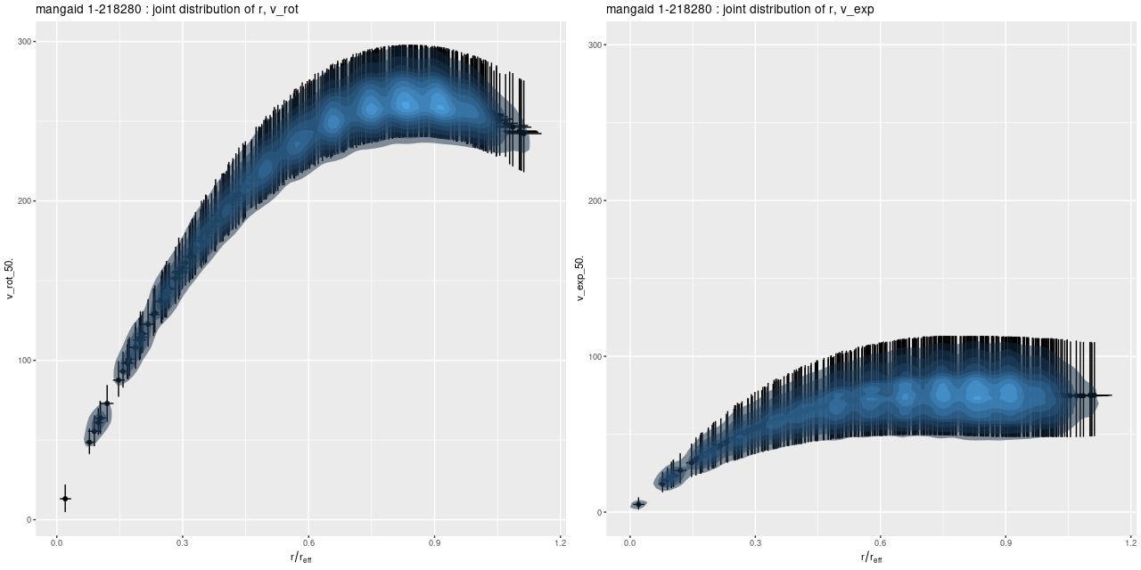
We need a single estimate of circular velocity. Since I scaled the coordinates by 1/(1.5Reff) the sum of the polynomial coefficients conveniently estimates the circular velocity at 1.5Reff, so that’s what I used. And here’s what I got (this is a log-log plot):
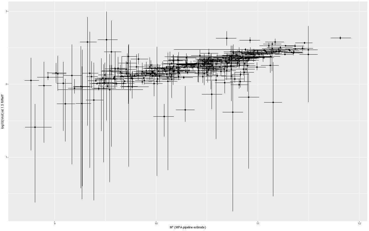
So, most points do follow a fairly tight linear relationship, but some measurements have very large error bars, and there are perhaps some outliers. The obvious choice to quantify the relationship, namely a simple linear regression with measurement error in both variables is also the wrong choice, I think. The reason is it’s not clear what the predictor should be, which suggests that we should be modeling the joint distribution rather than a conditional distribution of one variable given the other. To do that I turn to what astronomers call “extreme deconvolution” (Bovy, Hogg, and Roweis 2009, 2010). This is another latent variable model where the observed values are assumed drawn from some distribution with unknown (latent) mean and known variances, and the latent variables are in turn modeled as being drawn from a joint distribution with mean and variance parameters to be estimated. Bovy et al. allowed the joint distribution to be a multiple component mixture. I wrote my own version in Stan, and for simplicity just allow a single component for now. The full code is listed at the end of this post. Another simplification I make is modeling the measurement errors as Gaussian, which is clearly not the case for at least some measurements since some error bars are asymmetric — the plotted error bars mark the 16th and 84th percentiles of log stellar mass (\(\approx \pm 1 \sigma\)) and 2.5th and 97.5th percentiles of log circular velocity (\(\approx \pm 1.96 \sigma\)). If I had more accurate distribution functions it would be straightforward to adjust the model. This should be feasible for the velocities at least since the rotation model outputs can be recovered and the empirical posteriors examined. The stellar mass estimates would be more difficult with only a few quantiles tabulated. But, forging ahead, here is the important result:
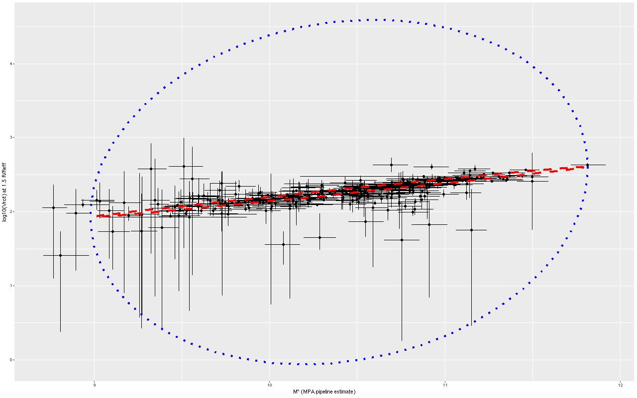
The skinny ellipse is a 95% confidence bound for the XD estimate of the intrinsic relationship. The fat ellipse is a 95% confidence ellipse for the posterior predictive distribution, which is obtained by generating new simulated observations from the full model. So there are two interesting results here. First, the inferred intrinsic relationship shows remarkably little “cosmic scatter,” consistent with a nearly perfect correlation between the unobserved true stellar mass and circular velocity. Second, it’s not at all clear that the apparent outliers are actually discrepant given the measurement error model.
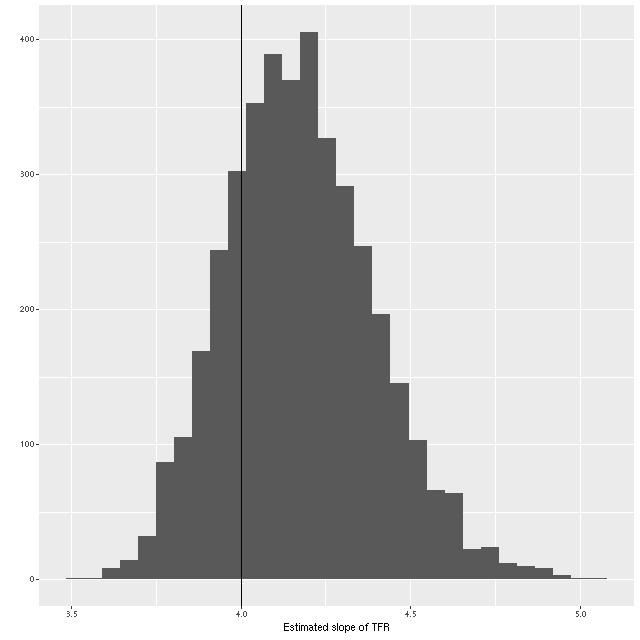
What about the slope of the relation? We can estimate that from the elements of eigenvectors of the eigendecomposition of the variance matrix, which I calculate in the generated quantities block of the Stan model. A histogram of the result is shown below. Although a slightly higher slope is favored, the McGaugh et al. value of 4 is well within the 95% confidence band.
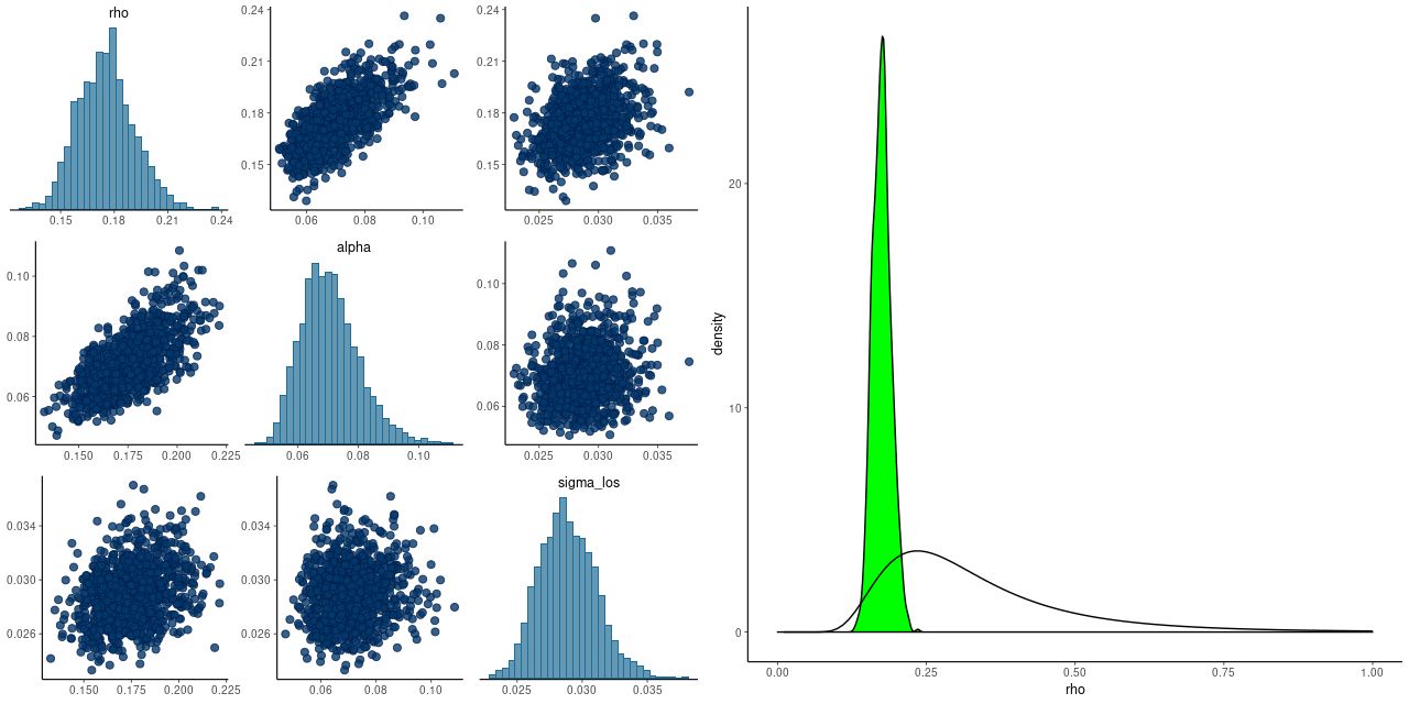
As a check on my model I compared my results to the implementation of the Bovy et al. algorithm in the Python module astroML that accompanies the book “Statistics, Data Mining, and Machine Learning in Astronomy” by Ivezic et al. (2014).
Here is my estimate of the mean of the posterior means of the intrinsic distribution (which isn’t especially interesting) and the posterior variance matrix:
> colMeans(post$mu_unorm)
[1] 10.396068  2.267223
> apply(post$Sigma_unorm, c(2,3), mean)

             [,1]       [,2]
  [1,] 0.32363805 0.07767842
  [2,] 0.07767842 0.01876449
and the same returned by XDGMM
array([[10.39541753, 2.2668531 ]])
array([[[0.32092995, 0.07733682],
        [0.07733682, 0.01866578] ]])
I also tried multicomponent mixtures in XDGMM and found no evidence that more than one is needed. In particular it doesn’t favor a different relation at the low mass end or any higher variance components to cover the apparent outliers.
I plan to return to this topic later, perhaps after the next data release and perhaps using the GP model for rotation curves (or something else if I find a different modeling approach that works).
Continue reading “An application – the Baryonic Tully Fisher relation”
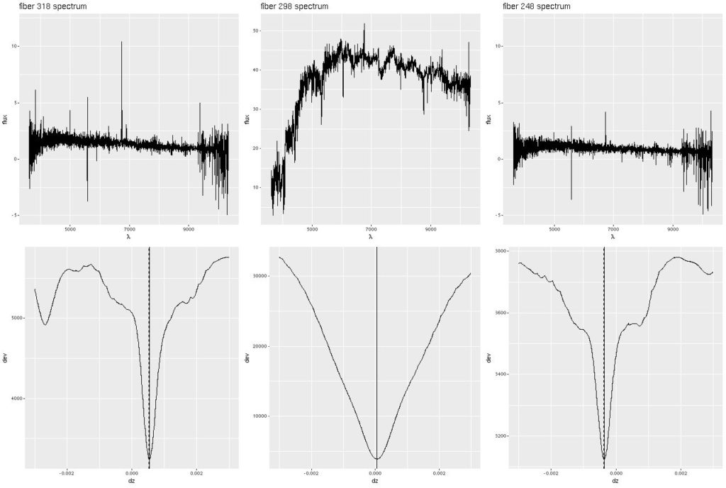 Deviance vs. delta z for 3 fiber/pointing combinations
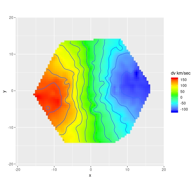
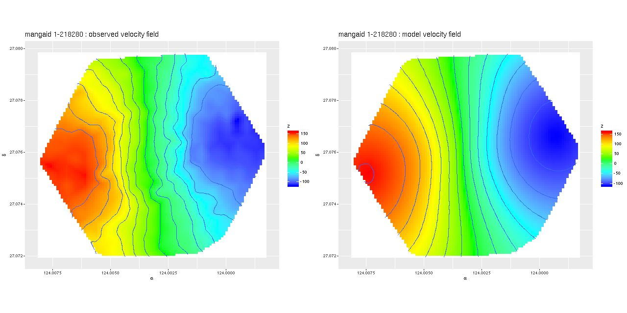
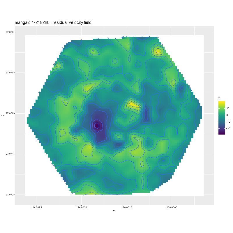
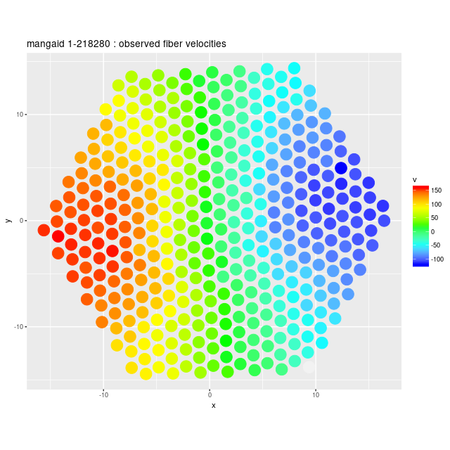 Example velocity field
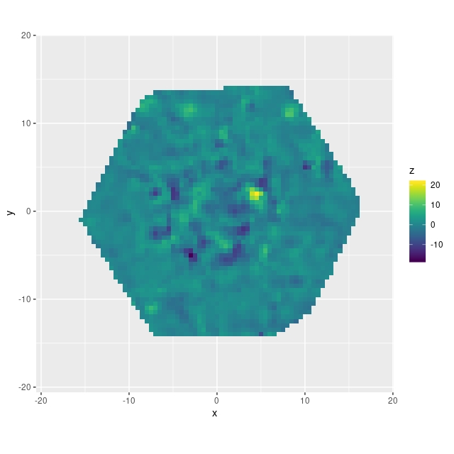
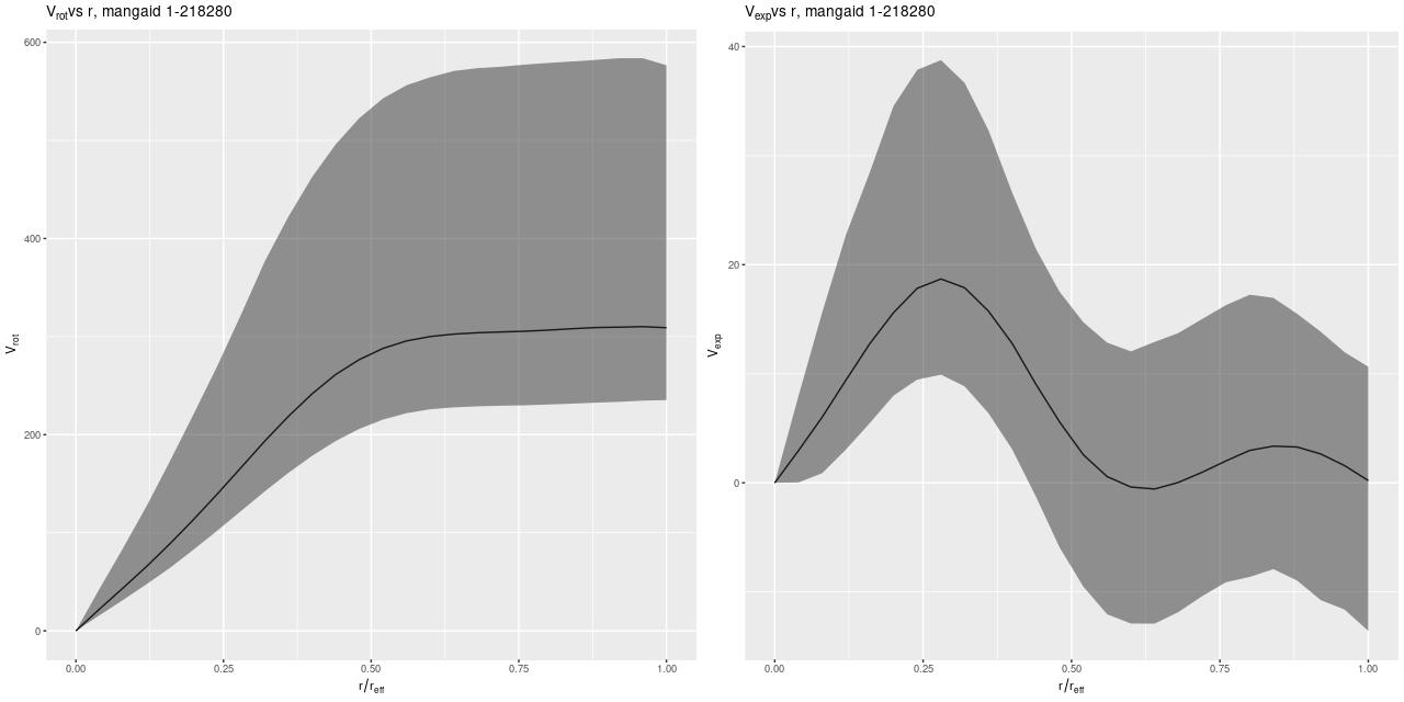
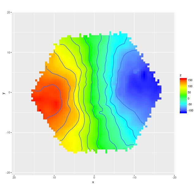 Example velocity field from data cube