SQL – Extragalactic

2020-12-272020-12-28

Using Galaxy Zoo classifications to select MaNGA samples

A while back I came across a paper by Fraser-McKelvie et al. (2020, arxiv id 2009.07859) that used Galaxy Zoo classifications to select a sample of barred spiral galaxies with MaNGA observations. This was a followup to a paper by Peterken et al. (2020, arxiv id 2005.03012) that also used Galaxy Zoo classifications to select a parent sample of spiral galaxies (barred and otherwise). There’s nothing new about using GZ classifications for sample selection of course, although these papers are somewhat notable for going farther down the decision tree than usual. What was new to me though when I decided to get my own samples is the SDSS CasJobs database now has a table named mangaGalaxyZoo containing GZ classifications for (I guess) all MaNGA galaxies. The classifications come from the Galaxy Zoo 2 database supplemented with some followup campaigns to fill in the gaps in GZ2. Besides greater completeness than the zoo2* database tables that can also be queried in CasJobs this table contains the newer vote fraction debiasing procedure described in Hart et al. (2016). It’s also much faster to query because it’s indexed on mangaid. When I put together the sample of MaNGA disk galaxies that I’ve posted about several times I took a somewhat indirect approach of looking for SDSS spectroscopic objects close to IFU centers and joining those with classifications in the zoo2MainSpecz table. The query I wrote took about 3 1/2 hours to execute, whereas the ones shown below required no more than a second.

Pasted below are the complete SQL queries, and below the fold are lists of the positions and plateifu IDs of the samples suitable for copying and pasting into the SDSS image list tool. These queries run in the DR16 “context” produced 287 and 272 hits respectively, with 285 unique galaxies in the barred sample and 263 uniques in the non-barred. These numbers are a little different than in the two papers referenced at the top. Fraser-McKelvie ended up with 245 galaxies in their barred sample — most of the difference appears to be due to me selecting from both the primary and secondary MaNGA samples, while they only used the “Primary+” sample (which presumably include the primary and “color enhanced” subsamples). I also did not make any exclusions based on the drp3qual value although I did record it. The total sample size of 548 galaxies is considerably smaller than the parent sample from Peterken, which was either 795 or 798 depending on which paper you consult. The main reason for that is probably that Peterken’s parent sample includes all bar classifications while I excluded galaxies with debiased f_bar levels > 0.2 in my bar-less sample. My barred fraction of around 52% is closer to guesstimates in the literature.

Both samples contain at least a few false positives, as is usual, but there are only one or two gross misclassifications. One that was especially obvious in the barred sample was this early type galaxy, which clearly has neither a bar or spiral structure and at least qualitatively has a brightness profile more characteristic of an elliptical. Oddly, the zoo2MainSpecZ entry for this object has a completely different set of classifications — the debiased vote fraction for “smooth” was 84%, so most volunteers agreed with me. This suggests maybe a misidentification in the mangaGalaxyZoo data.

Besides this really obvious case I found a few with apparent inner rings or lenses, and a few galaxies in both samples appear to me to be lenticulars with no clear spiral structure. The first of the two below again has a completely different set of classifications in zoo2MainSpecZ than in the MaNGA table.

Although I didn’t venture to count them a fair number of galaxies in the non-barred sample do appear to have short and varyingly obvious bars. Of course the query didn’t exclude objects with some bar votes — presumably higher purity could be achieved by lowering the threshold for exclusion. And again, there are a few lenticulars in the spiral sample. As my sadly departed friend Jean Tate often commented the galaxy zoo decision tree doesn’t lend itself very well to identifying lenticulars.

Unfortunately I have nothing useful to say about Fraser-Mckelvie’s main research topic, which was to decide if, and perhaps why, barred spirals have lower star formation rates than otherwise similar non-barred ones. 500+ galaxies are far more than I can analyze with my computing resources. Perhaps a really high purity sample would be manageable. I may post an individual example or two anyway. The MaNGA view of grand design spirals in particular can be quite striking.

select into gzbars
  m.mangaid,
  m.plateifu,
  m.plate,
  m.objra,
  m.objdec,
  m.ifura,
  m.ifudec,
  m.mngtarg1,
  m.drp3qual,
  m.nsa_z,
  m.nsa_zdist,
  m.nsa_elpetro_mass,
  m.nsa_elpetro_phi,
  m.nsa_elpetro_ba,
  m.nsa_elpetro_th50_r,
  m.nsa_sersic_n,
  gz.survey,
  gz.t01_smooth_or_features_count as count_features,
  gz.t01_smooth_or_features_a02_features_or_disk_debiased as f_disk,
  gz.t03_bar_count as count_bar,
  gz.t03_bar_a06_bar_debiased as f_bar,
  gz.t04_spiral_count as count_spiral,
  gz.t04_spiral_a08_spiral_debiased as f_spiral,
  gz.t06_odd_count as count_odd,
  gz.t06_odd_a15_no_debiased as f_notodd
from mangaDrpAll m
join mangaGalaxyZoo gz on gz.mangaid = m.mangaid
where
  m.mngtarg2=0 and
  gz.t04_spiral_count >= 20 and
  gz.t03_bar_count >= 20 and
  gz.t01_smooth_or_features_a02_features_or_disk_debiased > 0.43 and
  gz.t03_bar_a06_bar_debiased >= 0.5 and
  gz.t04_spiral_a08_spiral_debiased > 0.8 and
  gz.t06_odd_a15_no_debiased > 0.5 and
  m.nsa_elpetro_ba >= 0.5 and
  m.mngtarg1 >= 1024 and
  m.mngtarg1 < 8192
order by m.plateifu

select into gzspirals
  m.mangaid,
  m.plateifu,
  m.plate,
  m.objra,
  m.objdec,
  m.ifura,
  m.ifudec,
  m.mngtarg1,
  m.drp3qual,
  m.nsa_z,
  m.nsa_zdist,
  m.nsa_elpetro_mass,
  m.nsa_elpetro_phi,
  m.nsa_elpetro_ba,
  m.nsa_elpetro_th50_r,
  m.nsa_sersic_n,
  gz.survey,
  gz.t01_smooth_or_features_count as count_features,
  gz.t01_smooth_or_features_a02_features_or_disk_debiased as f_disk,
  gz.t03_bar_count as count_bar,
  gz.t03_bar_a06_bar_debiased as f_bar,
  gz.t04_spiral_count as count_spiral,
  gz.t04_spiral_a08_spiral_debiased as f_spiral,
  gz.t06_odd_count as count_odd,
  gz.t06_odd_a15_no_debiased as f_notodd
from mangaDrpAll m
join mangaGalaxyZoo gz on gz.mangaid = m.mangaid
where
  m.mngtarg2=0 and
  gz.t04_spiral_count >= 20 and
  gz.t03_bar_count >= 20 and
  gz.t01_smooth_or_features_a02_features_or_disk_debiased > 0.43 and
  gz.t03_bar_a06_bar_debiased <= 0.2 and
  gz.t04_spiral_a08_spiral_debiased > 0.8 and
  gz.t06_odd_a15_no_debiased > 0.5 and
  m.nsa_elpetro_ba >= 0.5 and
  m.mngtarg1 >= 1024 and
  m.mngtarg1 < 8192
order by m.plateifu

2019-12-062019-12-06

Selecting “transitioning” galaxies

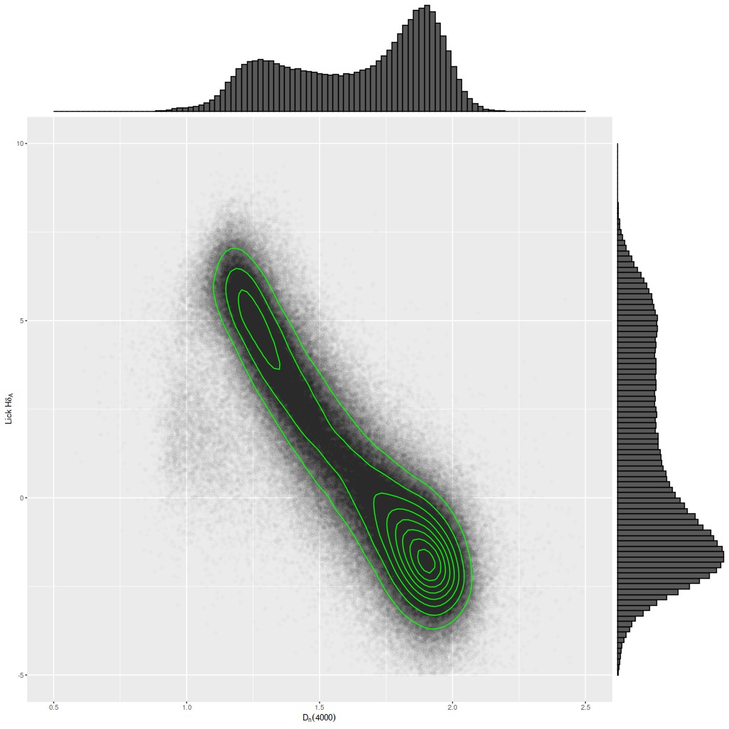
I’ve mentioned a few times that I took a shot several years ago at selecting a sample of post-starburst, or to use a term that’s gained some currency recently, “transitioning” galaxies¹ One thing that astronomers have come to realize is that traditional K+A spectroscopic selection criteria (basically requiring a combination of strong Balmer absorption lines and weak emission) potentially miss important populations, for example galaxies hosting an AGN. Selecting for weak emission also implies that star formation has already shut down, which precludes finding galaxies that are in the process of shutting down but still forming stars. On the other hand simply dropping constraints on emission won’t work because the resulting sample would be contaminated with a large fraction of normal star forming galaxies. Here is a popular spectroscopic diagnostic diagram, plotting the (pseudo) Lick Hδ_A index against the 4000Å break strength index D_n(4000). This version used the MPA-JHU measurements for approximately 1/2 of SDSS single fiber galaxy spectra from DR8.

hd_d4000_380K_mpa_jhu — The lick Hδ – 4000Å break strength plane for a large sample of SDSS galaxies. Measurements from the MPA-JHU pipeline.

As is true of many observed properties of galaxies the distribution in this diagram is strongly bimodal, with one of the modes centered right around Hδ_A ≈ 5Å. For the most part this region of the Hδ-D4000 plane is occupied by starforming galaxies — somewhere around 8-10% of all SDSS spectra with MPA measurements have Hδ_A ≥ 5Å, while true K+A galaxies are no more than a fraction of a percent of the local population. I took the simplest possible approach to try to minimize contamination from starforming galaxies: besides a traditional K+A selection with slightly relaxed emission line constraints I made a selection of spectra with emission line ratios in the “other than starforming” region of the [N II]/Hα vs [O III]/Hβ BPT diagnostic. I decided to use Kauffmann’s empirical starforming boundary as the selection criterion, and therefore included the so-called “composite” region of the BPT diagnostic. For the sake of completeness and reproducibility here is part of the CASJobs query I used. I saved a number of measurements from the MPA spectroscopic pipeline as well as the SDSS photo pipeline that aren’t included in the listing below. I did include a few lines just to point out that it’s important to use the emission line subtracted version of the Lick Hδ index because it can be significantly contaminated. Most of the where clause of the query is selecting spectra with firm detections and good error estimates of the relevant emission and absorption lines. There is also a redshift range constraint — the upper limit is set to avoid contamination of Hδ by the 5577Å terrestrial night sky line. Finally there are some modest quality constraints.

select into mydb.kaufpostagn
  gi.lick_hd_a_sub as lick_hd_a,
  gi.lick_hd_a_sub_err as lick_hd_a_err,
  gi.d4000_n,
  gi.d4000_n_err
from specObj s
  left outer join PhotoObj as p on s.bestObjid = p.Objid
  left outer join galSpecline as g on s.specObjid = g.specObjid
  left outer join galSpecIndx as gi on s.specObjid = gi.specObjid
  left outer join galSpecExtra as ge on s.specObjid = ge.specObjid
  where
  (g.h_alpha_flux/g.h_alpha_flux_err > 3 and g.h_alpha_flux_err > 0) and
  (g.nii_6584_flux/g.nii_6584_flux_err > 3 and g.nii_6584_flux_err > 0) and
  (g.h_beta_flux/g.h_beta_flux_err > 3 and g.h_beta_flux_err > 0) and
  (g.oiii_flux/g.oiii_flux_err > 3 and g.oiii_flux_err > 0) and
  ((0.61/(log10(g.nii_6584_flux/g.h_alpha_flux)-0.05)+1.3 < 
    log10(g.oiii_flux/g.h_beta_flux)) or (log10(g.nii_6584_flux/g.h_alpha_flux)>=0.05)) and
  (gi.lick_hd_a_sub > 5 and gi.lick_hd_a_sub_err > 0) and
  (s.z > .02 and s.z < 0.35) and
  (s.snMedian > 10) and
  (s.zWarning = 0 or s.zWarning = 16)
  order by
  s.plate, s.mjd, s.fiberid

I used a second query to make a more traditional K+A selection. This all could have been done with a single query but the conditions get a bit complicated. These queries run in the DR10 “context”² should return 4,235 and 874 hits respectively, with some overlap.

select into mydb.myka
s.ra,
s.dec,
s.plate,
s.mjd,
s.fiberid,
s.specObjid,
from specObj s
left outer join PhotoObj as p on s.bestObjid = p.Objid
left outer join galSpecline as g on s.specObjid = g.specObjid
left outer join galSpecIndx as gi on s.specObjid = gi.specObjid
left outer join galSpecExtra as ge on s.specObjid = ge.specObjid
where
  (g.oii_3729_eqw > -5 and g.oii_3729_eqw_err > 0) and
  (g.h_alpha_eqw >  -5 and g.h_alpha_eqw_err > 0) and
  (gi.lick_hd_a_sub > 5 and gi.lick_hd_a_sub_err > 0) and
  (s.z > .02 and s.z < 0.35) and
  (s.snMedian > 10) and
  (s.zWarning = 0 or s.zWarning = 16)
order by
  s.plate, s.mjd, s.fiberid

I thought at the time based solely on examining SDSS thumbnails that there were rather too many false positives in the form of normal starforming galaxies for the intended purpose of the sample. The choice to include galaxies in Kauffmann’s composite region played some role in this — although even the people responsible for this classification scheme admit now that it’s too simple some galaxies really do have spectra that are composites of starforming regions and AGN. But the more important reason I think is the well known problem that single fiber spectra only cover a portion of most nearby galaxies and galaxy nuclei (which were the intended targets) just aren’t representative of the global properties of galaxies. The SPOGS³ sample of Alatalo et al. 2016, which has similar aims to my selection but more elaborate selection criteria, has (in my opinion) a similar issue of false positives for the same reason.

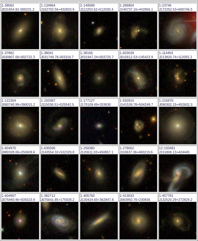
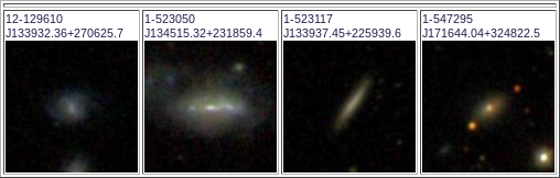
MaNGA provides a unique opportunity to examine the causes of false positives in my transitional sample, and I hope also confirm some real positives. A simple position crossmatch of my sample, which has about 5500 members, with MaNGA DR15 object coordinates produced 29 matches with a position tolerance of about 3″. SDSS thumbnails of the 29 are shown below. By my count at least 13, or 45%, of the sample are visibly disturbed in some way with 7 of those being clear merger remnants with evident shells and tidal tails.

I’ve been calculating star formation history models for these at a leisurely pace and plan to write more about the sample in future posts. Two of these I’ve already written about — besides Mrk 848 number 15 in the postage stamps was the subject of a series of posts starting here. I may write more case studies like those, or perhaps take a more holistic look at the sample and compare to a control group.

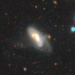
As something of an aside, with a looser position matching tolerance a 30th object turns up:

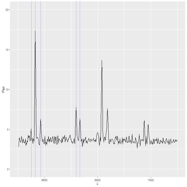
This made my sample based on the spectrum of the eastern nucleus. This object turns out to be doubly strange. Besides having two apparent nuclei, when I did some preliminary spectral fitting I noticed a peculiar pattern of residuals that turned out to be due to this:

8083-9101_spec_extract — Extract from a single spectrum of plateifu 8083-9101 (mangaid 1-38017)

Many of the spectra have emission lines at exactly their rest frame wavelengths. This particular spectrum, which came from somewhere in the SE quadrant of the IFU footprint, clearly shows Hα plus the [N II] and [S II] doublets offset from the same lines at the redshift of the galaxy. It turns out this galaxy lies near the edge of the Orion-Eridanus superbubble, a large region of diffuse emission in our galaxy. Should I choose to study this galaxy in more detail these lines could be masked easily enough, but the metadata for this data cube says it shouldn’t be used.

2018-07-30

An application – the Baryonic Tully Fisher relation

Automating the processing of rotation curve models for the sample I described in the previous post was a relatively straightforward exercise. I just wrote a short script to load the galaxy data, estimate the velocity field, and run the Stan model for the entire sample. I use the MaNGA catalog values of nsa_elpetro_ph and nsa_elpetro_ba as proxies for the major axis position angle and cosine of inclination. Recall from a few posts back that these are used both to set priors for the corresponding model parameters and to initialize the sampler. There’s a small problem in that the photometric major axis is defined modulo \(\pi\) while the kinematic position angle is measured modulo \(2 \pi\). A 180^o error here just causes the signs of the polynomial coefficients for rotation velocity to flip, which is easily corrected in post-processing.

I also use the catalog value nsa_elpetro_th50_r as the estimate of the effective radius, rescaling the input coordinates by dividing by 1.5r_eff. To save future processing (and also as insurance against power outages, etc.) all of the relevant input data and model fits are saved to an R binary data file for each galaxy. This all took some days for this sample, with the most time consuming operation being the calculation of the velocity fields.

Not all of the model runs were successful. Foreground stars and galaxy overlaps can cause catastrophic errors in the velocity offset measurements, and just one such error can seriously skew the rotation curve model. For these cases I manually masked the offending spectra and reran the models. There were three other sources of model failure: a single case of a bulge dominated galaxy, galaxies that were too nearly face on to reliably measure rotation, and galaxies with large kinematic misalignments (that is where the direction of maximum recession velocity is significantly offset from the photometric major axis). I will discuss these cases and what I did about them in more detail in a later post. For now it suffices to say I ended up with 331 galaxies with satisfactory rotation curve estimates.

With rotation curves in hand I decided as a simple project to try to replicate the Baryonic Tully Fisher relation. In its original form (Tully and Fisher 1977) the TFR is a relationship between circular velocity measured at some fiducial radius and luminosity, and as such it constitutes a tertiary distance indicator. Since stellar mass follows light (more or less) it makes sense that a similar relationship should hold between circular velocity and mass, and in due course this was found to be the case by McGaugh et al. (2000) who found \(M_b \sim V_c^4\) over a 5 decade range in baryonic (that is stellar plus gas) mass.

I retrieved stellar masses from the MPA-JHU (and also Wisconsin) pipeline using the following query:


select into gz2diskmass
  gz.mangaid,
  gz.plateifu,
  gz.specObjID,
  ge.lgm_tot_p16,
  ge.lgm_tot_p50,
  ge.lgm_tot_p84,
  w.mstellar_median,
  w.mstellar_err
from mydb.gz2disks gz
left outer join galSpecExtra ge on ge.specObjID = gz.specObjID
left outer join stellarMassPCAWiscBC03 w on w.specObjID = gz.specObjID

The MPA stellar mass estimates were from a Bayesian analysis, and several quantiles of the posterior are tabulated. I use the median as the best estimate of the central value and the 16th and 84th percentiles as \(\pm 1\sigma\).

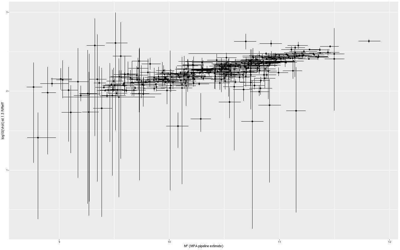
We need a single estimate of circular velocity. Since I scaled the coordinates by 1/(1.5R_eff) the sum of the polynomial coefficients conveniently estimates the circular velocity at 1.5R_eff, so that’s what I used. And here’s what I got (this is a log-log plot):

tf_mv — Stellar mass vs. rotation velocity at 1.5Reff for 331 disk galaxies

So, most points do follow a fairly tight linear relationship, but some measurements have very large error bars, and there are perhaps some outliers. The obvious choice to quantify the relationship, namely a simple linear regression with measurement error in both variables is also the wrong choice, I think. The reason is it’s not clear what the predictor should be, which suggests that we should be modeling the joint distribution rather than a conditional distribution of one variable given the other. To do that I turn to what astronomers call “extreme deconvolution” (Bovy, Hogg, and Roweis 2009, 2010). This is another latent variable model where the observed values are assumed drawn from some distribution with unknown (latent) mean and known variances, and the latent variables are in turn modeled as being drawn from a joint distribution with mean and variance parameters to be estimated. Bovy et al. allowed the joint distribution to be a multiple component mixture. I wrote my own version in Stan, and for simplicity just allow a single component for now. The full code is listed at the end of this post. Another simplification I make is modeling the measurement errors as Gaussian, which is clearly not the case for at least some measurements since some error bars are asymmetric — the plotted error bars mark the 16th and 84th percentiles of log stellar mass (\(\approx \pm 1 \sigma\)) and 2.5th and 97.5th percentiles of log circular velocity (\(\approx \pm 1.96 \sigma\)). If I had more accurate distribution functions it would be straightforward to adjust the model. This should be feasible for the velocities at least since the rotation model outputs can be recovered and the empirical posteriors examined. The stellar mass estimates would be more difficult with only a few quantiles tabulated. But, forging ahead, here is the important result:

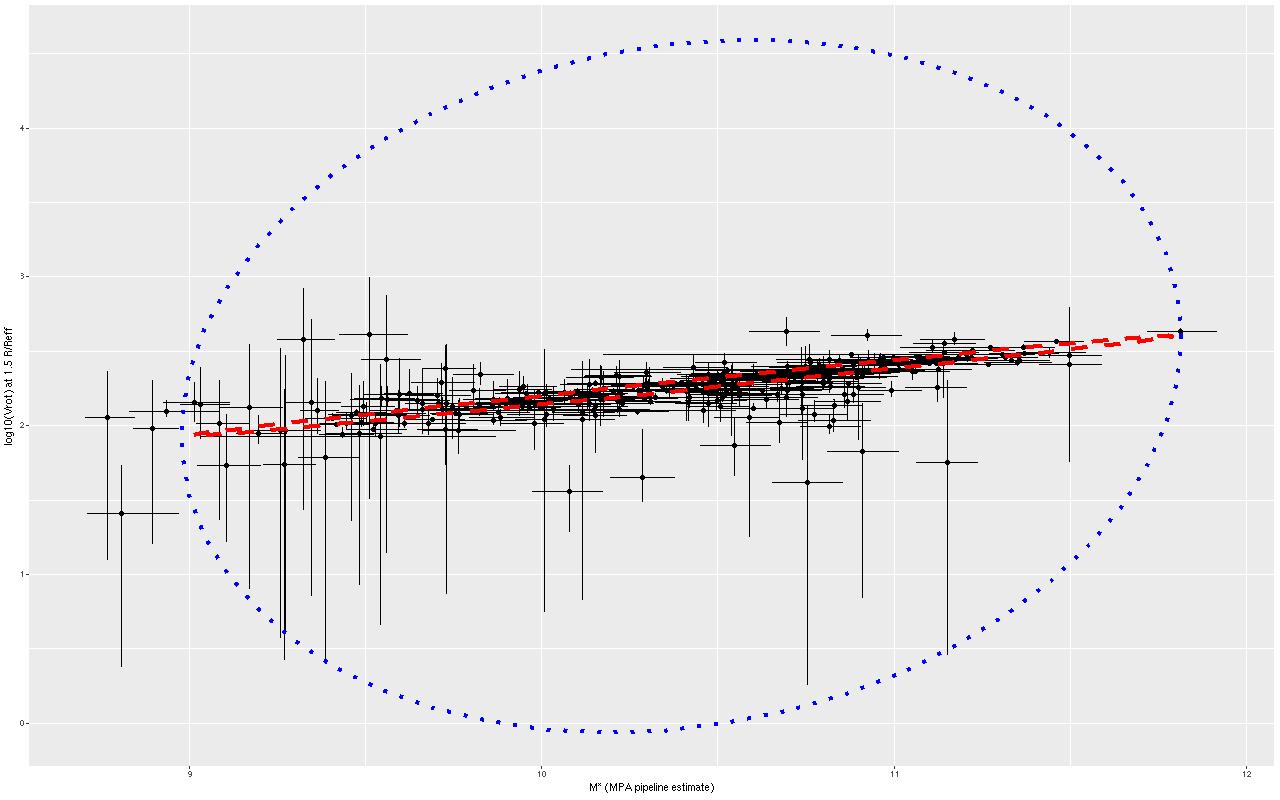
tf_mv_confellipse — Stellar masses vs. rotation velocity with 95% confidence ellipses for “extreme deconvolution” estimate of relationship and pp distribution

The skinny ellipse is a 95% confidence bound for the XD estimate of the intrinsic relationship. The fat ellipse is a 95% confidence ellipse for the posterior predictive distribution, which is obtained by generating new simulated observations from the full model. So there are two interesting results here. First, the inferred intrinsic relationship shows remarkably little “cosmic scatter,” consistent with a nearly perfect correlation between the unobserved true stellar mass and circular velocity. Second, it’s not at all clear that the apparent outliers are actually discrepant given the measurement error model.

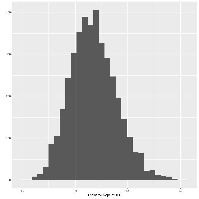
What about the slope of the relation? We can estimate that from the elements of eigenvectors of the eigendecomposition of the variance matrix, which I calculate in the generated quantities block of the Stan model. A histogram of the result is shown below. Although a slightly higher slope is favored, the McGaugh et al. value of 4 is well within the 95% confidence band.

tfr_slope — Estimate of the slope of the TFR

As a check on my model I compared my results to the implementation of the Bovy et al. algorithm in the Python module astroML that accompanies the book “Statistics, Data Mining, and Machine Learning in Astronomy” by Ivezic et al. (2014).

Here is my estimate of the mean of the posterior means of the intrinsic distribution (which isn’t especially interesting) and the posterior variance matrix:

> colMeans(post$mu_unorm)
[1] 10.396068  2.267223
> apply(post$Sigma_unorm, c(2,3), mean)
      
             [,1]       [,2]
  [1,] 0.32363805 0.07767842
  [2,] 0.07767842 0.01876449

and the same returned by XDGMM

array([[10.39541753,  2.2668531 ]])

array([[[0.32092995, 0.07733682],
        [0.07733682, 0.01866578] ]])

I also tried multicomponent mixtures in XDGMM and found no evidence that more than one is needed. In particular it doesn’t favor a different relation at the low mass end or any higher variance components to cover the apparent outliers.

I plan to return to this topic later, perhaps after the next data release and perhaps using the GP model for rotation curves (or something else if I find a different modeling approach that works).
Continue reading “An application – the Baryonic Tully Fisher relation”

2018-07-21

Sample selection – finding disk galaxies

This post is partially based on a series I wrote on the previous version of Galaxy Zoo Talk. I hope it will be shorter.

The analysis in the previous posts is applicable to galaxies whose stars and/or ionized gas are confined to a thin disk with no net vertical bulk motion. In that case velocities can be treated as two dimensional and, for moderately inclined disks, the full velocity vectors recovered from the observed radial velocities. The thin disk approximation is an idealization of course, but it’s reasonable at least for late type spiral galaxies that lack significant bulges.

I ultimately tried three different ideas to acquire a statistically meaningful sample of disk galaxies without actually visually examining all ∼2700 of them (this is certainly feasible, but somewhat error prone and tedious). The first idea was to use the drpall catalog to select a sample of probable disk galaxies. The catalog contains a single morphology proxy in nsa_sersic_n derived from single component sersic index fits to r-band SDSS imaging. A forgotten paper suggests disk galaxies have n ≤ 2.5, so I adopted that as an upper limit. There are several estimates of the minor to major axis size ratio, which for a disk galaxy is a proxy for the cosine of the inclination. The one recommended by the MaNGA science team is nsa_elpetro_ba. I chose a conservative range of inclinations of between 30 and 60^o, or \(0.5 \le \cos i \le 0.866\).

The full MaNGA sample contains several subsamples: the main ones are a primary sample intended to be observed out to ≈1.5 effective radii and a secondary sample observed to ≈2.5R_eff. I initially thought the latter would be most suitable for analysis. The subsample an observation belongs to is identified by three sets of bitmasks, with mngtarg1 used for galaxies in the primary and secondary samples. So, the R code to select this sample is:


attach(drpcat)
maybedisks2 <- which((mngtarg1==4 | mngtarg1==32 | (mngtarg1 >= 2048 & mngtarg1 < 4096)) & nsa_sersic_n < 2.5 & nsa_elpetro_ba>=0.5 & nsa_elpetro_ba<=0.866)
detach(drpcat)

This returns a vector of 254 row indexes in drpcat (in the DR14 release). The following short R function takes the indexes and writes out a text file of MaNGA file names suitable for use with wget


writefn <- function(indexes, ftype="rss", cat=drpcat, outfile="fgets.txt") {
  ftype <- toupper(ftype)
  plates <- cat$plate[indexes]
  plateifus <- cat$plateifu[indexes]
  fnames <- paste(plates, "/stack/manga-", plateifus,
                  "-LOG", ftype, ".fits.gz", sep="")
  cat(fnames, file=outfile, sep="\n")
  fnames
}

I soon found out that this sample has problems. The main issue is that although the IFU covers almost the full visible extent of these galaxies the exposures are no deeper than for the primary sample. Even with optimistic S/N thresholds there is little usable data at large radii.

My next idea was to try the very pure sample of spirals of Masters et al. (2010) selected from the original Galaxy Zoo project. A position cross-reference turned up 69 observations of 68 unique galaxies in the first two MaNGA releases. This is a bit small for the purpose I had in mind, and the sample size was further reduced by another 10-12 galaxies that were too nearly face-on to analyze.

In search of a larger sample I again turned to Galaxy Zoo data, this time the main spectroscopic sample of GZ2 (Willett et al. 2013) which is conveniently included in the SDSS databases. A complication here is that although the vast majority of MaNGA galaxies have single fiber spectra from SDSS their id's aren't tabulated in drpall. Although I could probably have done a simple position based cross match of GZ2 galaxies with MaNGA targets I decided instead to look for SDSS specObjID's near to MaNGA target positions, and then join to matching GZ2 targets. This required a command I hadn't used before and a table valued function that was also new to me:


select into gz2disks
  m.mangaid,
  m.plateifu,
  m.objra,
  m.objdec,
  m.ifura,
  m.ifudec,
  m.mngtarg1,
  m.mngtarg3,
  m.nsa_z,
  m.nsa_zdist,
  m.nsa_elpetro_phi,
  m.nsa_elpetro_ba,
  m.nsa_elpetro_th50_r,
  m.nsa_sersic_n,
  z.specObjID
from mangaDrpAll m
cross apply dbo.fGetNearbySpecObjEq(m.objra, m.objdec, 0.05) as n
join zoo2MainSpecz z on z.specobjid=n.specObjID
where
  m.mngtarg2=0 and
  z.t01_smooth_or_features_a02_features_or_disk_weighted_fraction > 0.5 and
  z.t02_edgeon_a05_no_weighted_fraction > 0.5 and
  z.t06_odd_a15_no_weighted_fraction > 0.5 and
  m.nsa_elpetro_ba >= 0.5 and
  m.nsa_elpetro_ba <= 0.866 and
  m.mngtarg1 > 0

The line that starts with cross apply builds a table of position matches of MaNGA objects to spectroscopic primaries, then in the next line joins data from the GZ2 spectroscopic sample. The last lines set some thresholds for weighted vote fractions for a few attributes: yes votes for "features or disk", no votes for "edge on", and no votes for "something odd". I chose, more or less arbitrarily, to set all thresholds to 0.5. The final lines set inclination proxy limits as discussed above. There were also questions about bulge size, spiral structure, and bars in the GZ2 decision tree that I did not consider but certainly might if I return to this subject.

This query run in the DR14 "context" produced 359 hits out of about 2700 galaxy targets in the first two MaNGA public releases, which is certainly an incomplete census of disk galaxies. On the other hand all 359 appeared to me actually to be disk galaxies, so the purity of the sample was quite high. Next time I'll do something with the sample.