January 2019 – Extragalactic

When I first began modeling disk galaxy rotation curves using low order polynomials for the circular velocity I noticed two rather frequent systematics in the model residuals:

Lobe like areas symmetrically located around the nucleus with approximately equal and opposite signs. Sometimes these are co-located with bar ends but a bar is not always obvious.
A contrast of a few 10’s of kilometers/sec between spiral arms and interarm regions. This is rather common in grand design spirals.

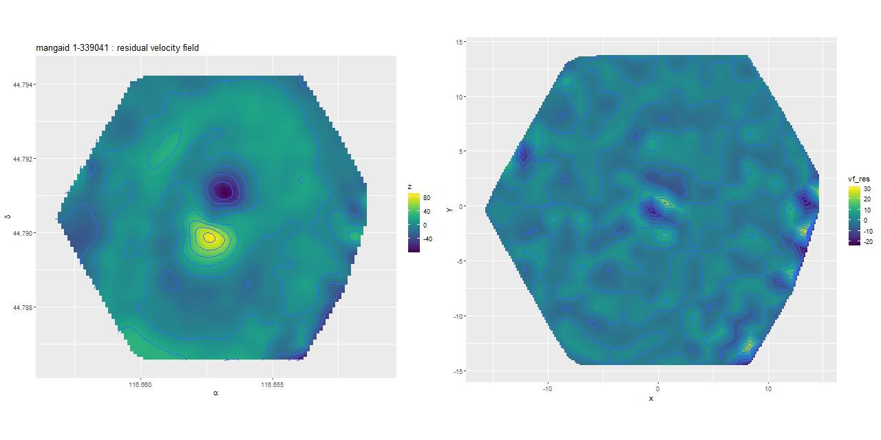
Here’s a particularly dramatic example of symmetrical lobes in mangaid 1-339041 (plateifu 8138-12704), IAU name SDSS J074637.70+444725.8. First, here are the measured line of sight velocities for the fiber spectra:

vf_rss_8138-12704 — (L) Velocity field measured from stacked RSS file (R) Interpolated velocity field mangaid 1-339041 (plateifu 8138-12704)

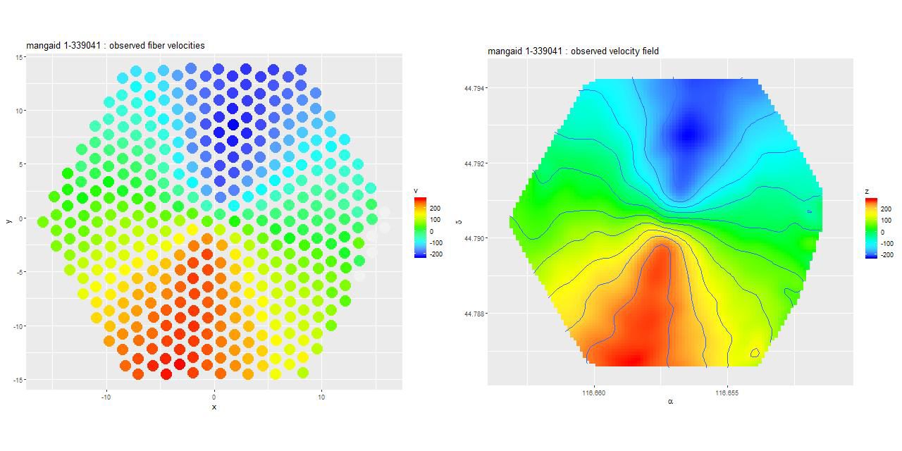
The left plot shows the actual measurements from the stacked RSS file. The right is just an interpolated version of the left. Since value added data is now available it’s worth comparing this to output from “Marvin“. For reference here is the Hα velocity map:

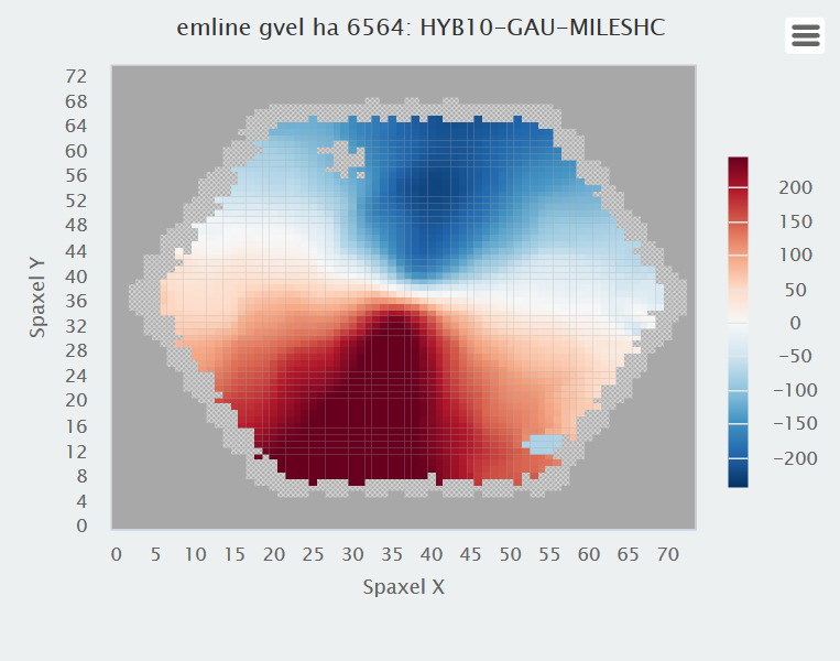
It’s hard to tell in any detail, but these look similar enough and the stellar velocity field as measured by the DAP also looks similar.

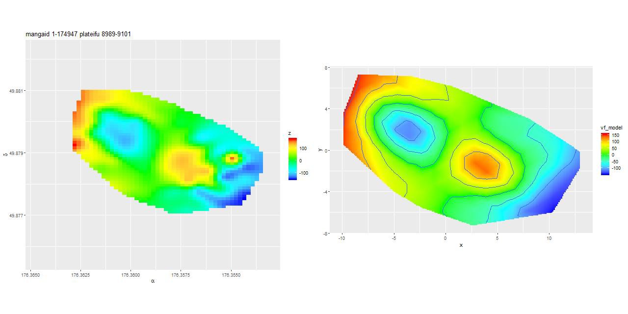
Next, here are the mean residuals from the posterior predictive fits shown as interpolated maps derived from the fits at the observed positions. As promised the left hand map from the low order polynomial fit has prominent lobes situated on either side of the nucleus and a more subtle contrast between spiral arms and interarm regions. The right hand map from the GP model appears to be largely free of systematic patterns. Why the difference?

vf_res_2ests_8138-12704 — Mean residuals from models: (L) Polynomial rotation curve model (R) GP model with atan mean function

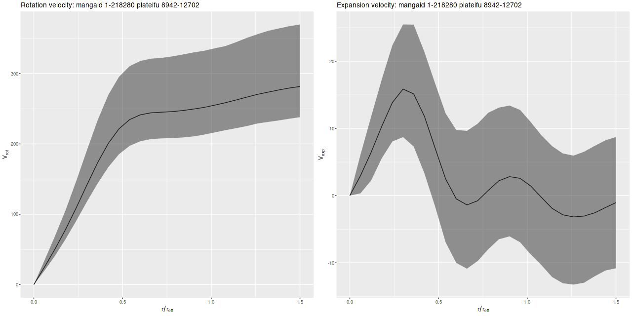
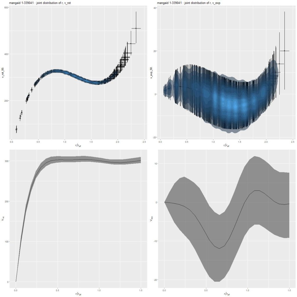
In this case the arctangent mean function I introduced in the last post worked very well, with the estimated circular velocity rising quickly to an asymptotic value of ∼300km/s. The low order polynomial representation is necessarily constrained by the possible shapes of a low order polynomial (in this case cubic), resulting in a shallower initial slope and a first local maximum farther out than in the GP model. The lobed residuals in the polynomial model are therefore seen to be due to an inner disk that’s rotating more rapidly than can be modeled (and not due to a kinematically distinct component or to streaming material).

rot_curves_2ests_8138-12704 — Rotation and “expansion” velocity curves (T) polynomial model (B) GP model with atan mean function

As a brief morphological note, GZ2 classifiers thought this was a normal looking disk galaxy by an overwhelming majority. It’s hard to say they were wrong based on the SDSS imaging, but the deeper and wider legacy survey thumbnail clearly shows the outer disk to be disturbed, presumably by the edge on disk galaxy to the north — the relative velocities are ∼340km/sec, so they are likely in close proximity.

As time allows I may take a closer look at model diagnostics available in Stan or some more examples. Longer term I plan to take another look at the Baryonic Tully-Fisher relationship for the larger sample available in DR15.

I haven’t had a lot of time for this hobby lately and won’t for another month or so, but I haven’t been completely inactive. When I first started modeling disk galaxy rotation curves with Gaussian processes I used a low order polynomial for the mean function. This was an admitted hack, and not a very good one at that. It’s not uncommon in the rotation curve modeling industry to adopt a functional form for the circular velocity. Sometimes it’s physically motivated (usually based on a bulge/disk/dark matter halo model), sometimes it’s purely phenomenological. With a bit of digging in the literature I found a particularly simple form in Courteau (1997):

\(v(r) = v_{0} + \frac{2}{\pi} v_{c} \arctan(r/r_{t})\)

Making this the mean function for the GP model involves just a few simple changes to the Stan code I outlined in that post. We only need two parameters for the curve, and the parameter block now looks like:

parameters {       
                
  real phi;       
                
  real<lower=0., upper=1.> cos_i;  // cosine disk inclination       
                
  real x_c;  //kinematic centers       
                
  real y_c;       
                
  real v_sys;     //system velocity offset (should be small)       
                
  real v_c;       
                
  real<lower=0> r_t;       
                
  real<lower=0.> sigma_los;       
                
  real<lower=0.> alpha;       
                
  real<lower=0.> rho;       
                
}

The key line in the model block is:

  v ~ multi_normal_cholesky(v_sys + sin_i * (2./pi() * v_c * atan(r/r_t) .* yhat ./ r), L_cov);

And then in the generated quantities block are posterior predictions for new data at the observed points and in concentric rings:

  // model and residuals at the original points       
                
         
                
  v_rot = 2./pi() * v_c * atan(r/r_t);       
                
  vf_model = gp_pred_rng(xyhat, v-v_sys-sin_i * (v_rot .* yhat ./ r), xyhat, alpha, rho, sigma_los);       
                
  vf_model = vf_model + v_sys + sin_i * (v_rot .* yhat ./r);       
                
  vf_res = v - vf_model;       
                
         
                
  // model in rings       
                
         
                
  v_gp = gp_pred_rng(xy_pred, v-v_sys-sin_i * (v_rot .* yhat ./ r), xyhat, alpha, rho, sigma_los);       
                
  v_pred = (v_gp + sin_i * 2./pi() * v_c * atan(r_pred/r_t) .* y_pred ./ r_pred) *v_norm/sin_i;       
                
  vrot_pred[1] = 0.;       
                
  vexp_pred[1] = 0.;

The full code is available in my github repository at https://github.com/mlpeck/vrot_stanmodels.

This model turned out to have very nice sampling properties using Stan’s version of NUTS, and convergence is fast enough in terms of both number of iterations and walltime to make it easily feasible to model a large sample.

Since I’ve been using this as a running example here are posterior circular and expansion velocity estimates for plateifu 8942-12702 (mangaid 1-218280):

gp_rot_exp_8942-12702 — Circular and Expansion velocities, mangaid 1-218280 estimated by GP model with atan mean function

These curves are shaped just slightly differently from the ones I posted in July, but the confidence bounds are somewhat tighter. Whether this is actually due to better inference remains to be seen.

Second topic: SDSS Data release 15 went public in December as promised. I haven’t had time to dig into it much, but I did rerun the query I used to get a sample of high confidence disk galaxies based on GZ2 classifications. Run in the DR15 context that query got 588 hits, an increase of 229 from DR14 and still about 13% of the entire MaNGA galaxy sample excluding ancillary targets that aren’t also part of the main samples.

I downloaded the RSS files and have done a first pass at rotation curve modeling of the 229 new galaxies. Unfortunately I won’t have time to actually analyze what I have until, most likely, March. To conclude for now here is the kinematically most interesting example I saw from the new to DR15 sample. GZ2 classifiers called this a normal disk galaxy by a large majority

and were about evenly divided on whether it has a bar. And here is its velocity field measured from the stacked RSS file on the left, with the modeled velocity field on the right. The left graph is interpolated to the same resolution as the data cubes.

vf_8989-9101 — Interpolated velocity field and GP based model, mangaid 1-174947 (plateifu 8989-9101)

This is an incomplete map because of the signal/noise threshold I set, but it’s apparent that the outer disk is counter-rotating relative to the inner disk. This is confirmed for the stellar velocity field in the SDSS DAP, while the ionized gas rotates in the same sense as the outer disk throughout. Keep in mind that I measure blended velocities that in any given case could be dominated either by stellar light or ionized gas — in this galaxy the emission lines are very weak, so I measured the stellar velocity field. The GP based model does a good job of fitting the data, but the rotation curve isn’t exactly the standard shape:

vrot_vexp_8989-9101 — Modeled circular and expansion velocity

One thing this demonstrates is the versatility of the gaussian process model with a simple mean function (even if it’s wrong).

Month: January 2019

Yet more on rotation curve modeling — why the mean function matters

Rotation curves revisited; SDSS DR15; miscellany