Well that was simple enough. I made a simple indexing error in the R data preprocessing code that resulted in a one pixel offset between the template and galaxy spectra, which effectively resulted in shifting the elements of the convolution kernel by one bin. I had wanted to look at a rotating galaxy to perform some diagnostic tests, but once I figured out my error this turned out to be a pretty good validation exercise. So I decided to make a new post. The galaxy I’m looking at is NGC 4949, another member of the sample of passively evolving Coma cluster galaxies of Smith et al. It appears to me to be an S0 and is a rapid rotator:
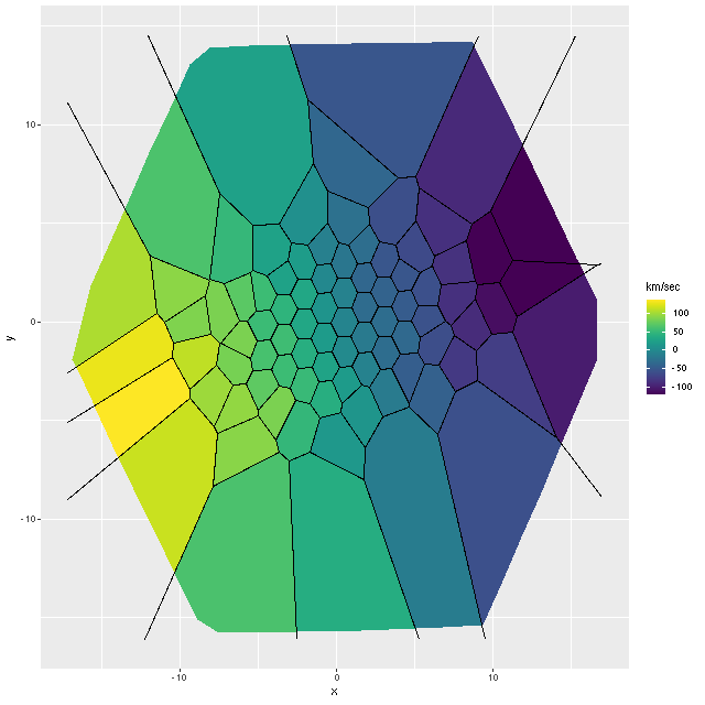
These projected velocities are computed as part of my normal workflow. I may in a future post explain in more detail how they’re derived, but basically they are calculated by finding the best redshift offset from the system redshift (taken from the NSA catalog which is usually the SDSS spectroscopic redshift) to match the features of a linear combination of empirically derived eigenspectra to the given galaxy spectrum.
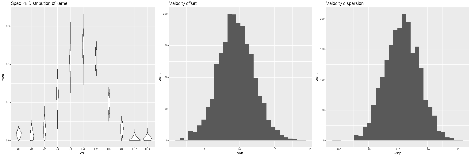
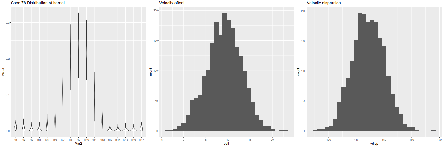
First exercise: find the line of sight velocity distribution after adjusting to the rest frame in each spectrum. This was the originally intended use of these models. This galaxy has fairly low velocity dispersion of ~100 km/sec. so I used a convolution kernel size of just 11 elements with 6 eigenspectra in each fit. Here is a summary of the LOSVD distribution for the central spectrum. This is much better. The kernel estimates are symmetrical and peak on average at the central element. The mean velocity offset is ≈ 9.5 km/sec, which is much closer to 0 than in the previous runs. I will look briefly at velocity dispersions at the end of the post: this one is actually quite close to the one I estimate with a single component gaussian fit (116 km/sec vs 110).
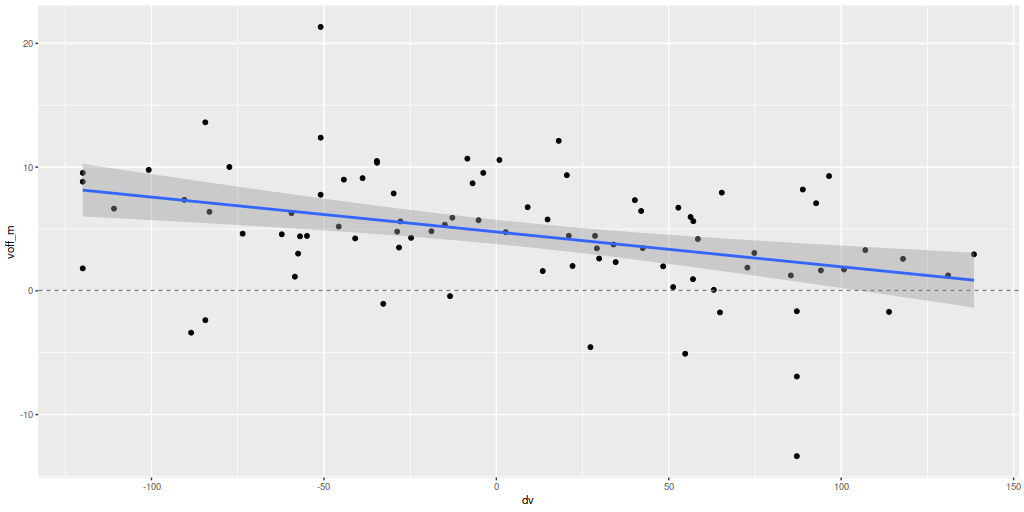
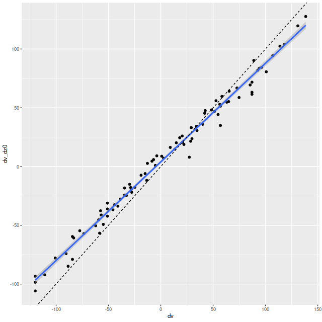
Next, here are the posterior mean velocity offsets for all 86 spectra in the Voronoi binned data, plotted against the peculiar velocity calculated as outlined above. The overall average of the mean velocity offsets is 4.6 km/sec. The reason for the apparent tilt in the relationship still needs investigation.
Exercise 2: calculate the LOSVD with wavelengths adjusted to the overall system redshift as taken from the NSA catalog, that is no adjustment is made for peculiar redshifts due to rotation. For this exercise I increased the kernel size to 17 elements. This is actually a little more than needed since the projected rotation velocities range over ≈ ± 100 km/sec. First, here is the radial velocity map:

Here’s a scatterplot of the velocity offsets against peculiar velocities from my normal workflow. Again there’s a slight tilt away from a slope of 1 evident. The residual standard error around the simple regression line is 6.4 km/sec and the intercept is 4 km/sec, which are consistent with the results from the first set of LOSVD models.
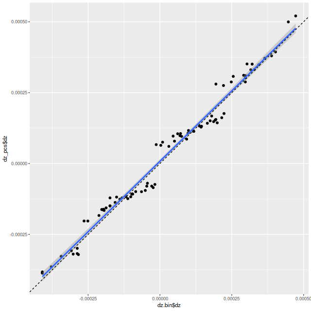
Exercise 3: calculate redshift offsets using a set of (for this exercise, 6) eigenspectra from the SSP templates. Here is a scatterplot of the results plotted against the redshift offsets from my usual empirically derived eigenspectra. Why the odd little jumps? I’m not completely sure, but my current code does an initial grid search to try to isolate the global maximum likelihood, which is then found with a general purpose nonlinear minimizer. The default grid size is 10-4, about the size of the gaps. Perhaps it’s time to revisit my search strategy.
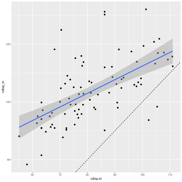
Final topic for now: I mentioned in the last post that posterior velocity dispersions (measured by the standard deviation of the LOSVD) were only weakly correlated with the stellar velocity dispersions that I calculate as part of my standard workflow. With the correction to my code the correlation while still weak has greatly improved, but the dispersions are generally higher:
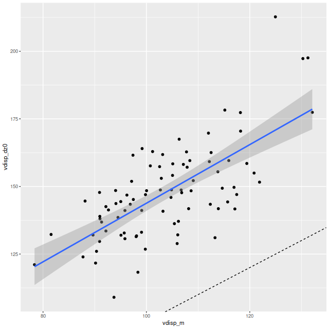
A similar trend is seen when I plot the velocity dispersions from the LOSVD models with correction only for the system redshift and a wider convolution kernel (exercise 2 above) with the fully corrected model runs (exercise 1):
These results hint that the diffuse prior on the convolution kernel is responsible for the different results. As part of the maximum likelihood fitting process I estimate the standard deviation of the stellar velocity distribution assuming it to be a single component gaussian. While the distribution of kernel values in the first graph look pretty symmetrical the tails are on average heavier than a gaussian. This can be seen too in the LOSVD models with the larger convolution kernel of exercise 2. The tails have non-negligible values all the way out to the ends:
Now, what I’m really interested in are model star formation histories. I’ve been using pre-convolved SSP model templates from the beginning along with phony emission line spectra with gaussian profiles with some apparent success. My plan right now is to continue that program with these non-parametric LOSVD’s. The convolutions could be carried out with posterior means of the kernel values or by drawing samples. Repeated runs could be used to estimate how much variation is affected by uncertainty in the kernel.
How to handle emission lines is another problem. For now stepping back to a simpler model (no emission, no dust) would be reasonable for this Coma sample.
