I only have time to analyze one MaNGA galaxy for now and since it was the first to get the correctly coded LOSVD estimates I chose the Coma Cluster S0 galaxy NGC 4949 that I discussed in the last post for SFH modeling. As I mentioned a few posts ago trying to model the LOSVD and star formation history simultaneously is far too computationally intensive for my resources, so for now I just convolve the SSP model spectral templates with the elementwise means of the convolution kernels estimated as described previously and feed those to the SFH modeling code. My intuition is that the SFH estimates should be at least slightly more variable if the kinematics are treated as variable as well, but for now there’s no real alternative to just picking a fiducial value. Of course a limited test of that hypothesis could be made by pulling multiple draws from the posterior of the LOSVD distribution. I will certainly try that in the future.
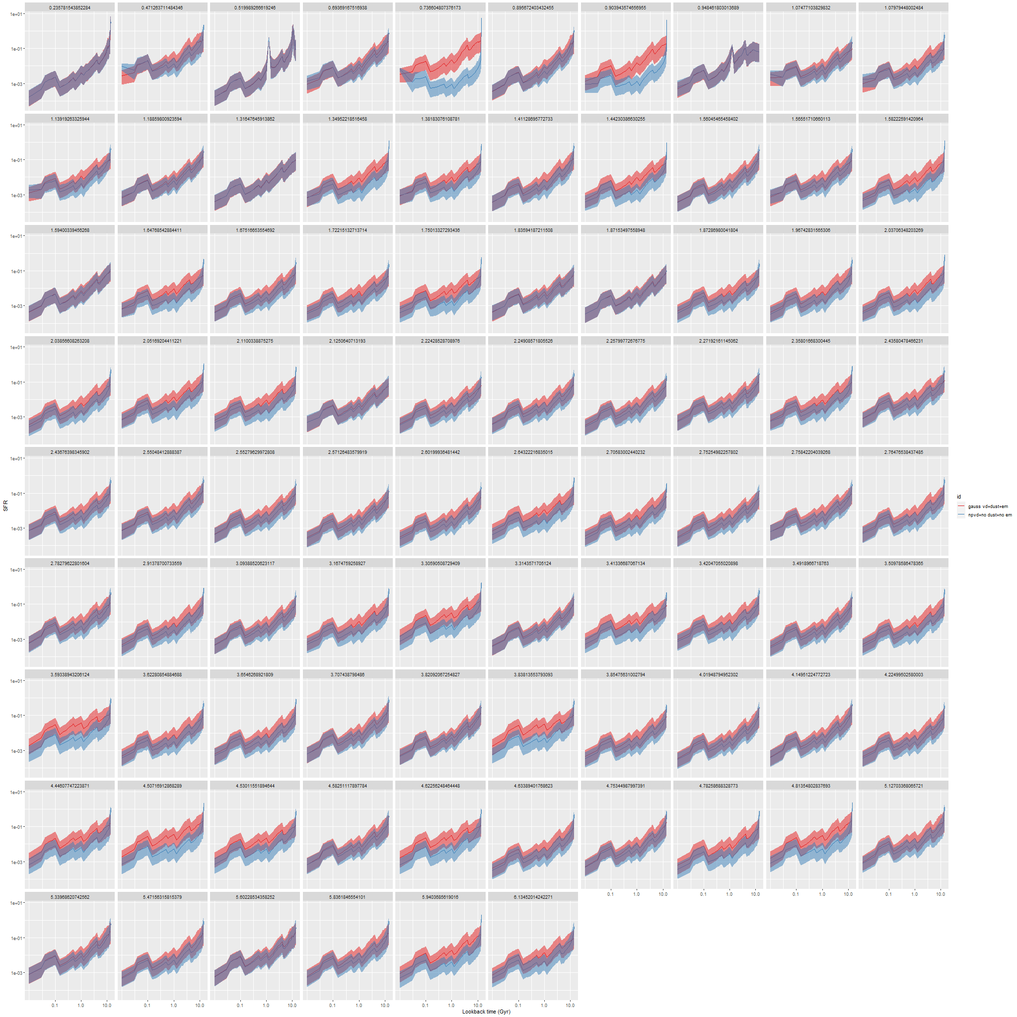
My first idea was to leave both dust and emission lines out of the SFH models. The first choice was to save CPU cycles and also based on the expectation that these passively evolving galaxies should have very little dust. The results were rather interesting: here are ribbon plots of model SFH’s for all 86 binned spectra. The pink ribbons are from the original model runs, which assumed single component gaussian velocity distributions, modified Calzetti attenuation, and included emission lines (which contribute negligible flux throughout). The blue ribbons are with non-parametric LOSVD and no attenuation model:
NGC 4949 – modeled star formation histories with single component gaussian and nonparametric estimates of line of sight velocity distributions with no dust model
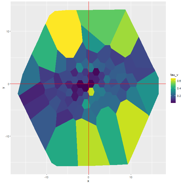
The differences in star formation histories turn out to be almost entirely due to neglecting dust in the second set of model runs. In this galaxy there are some areas with apparently non-negligible amounts of dust:
NGC 4949 – map of estimated optical depth of attenuation
Ignoring attenuation forces the model to use redder, hence older (and probably more metal rich although I haven’t yet checked) stellar populations and this has, in some cases, profound effects on the model SFH.
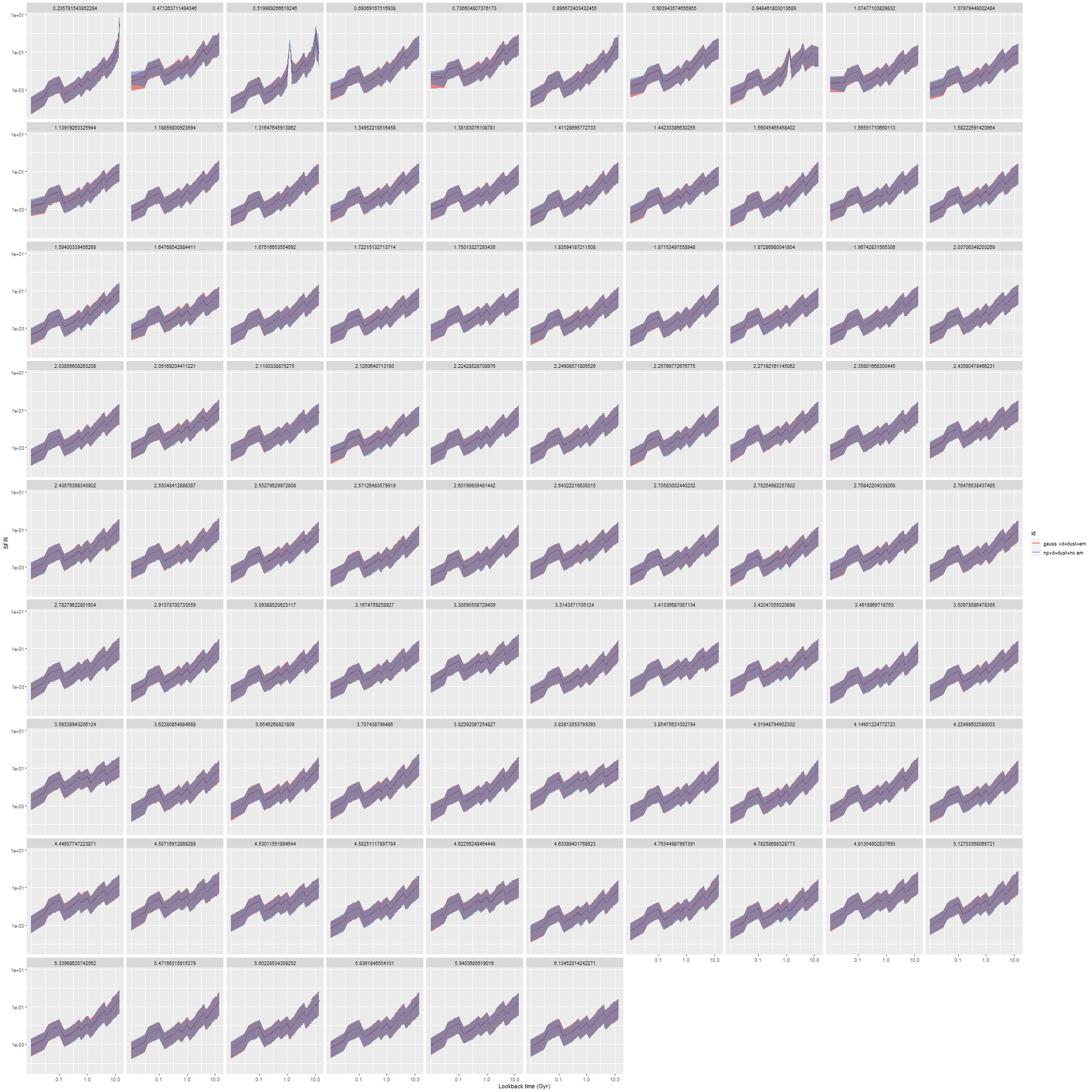
So, I tried a second set of model runs adding back in modified Calzetti attenuation but still leaving out emission:
NGC 4949 – modeled star formation histories with single component gaussian and nonparametric estimates of line of sight velocity distributions
And now the models are nearly identical, with minor differences mostly in the youngest age bin. All other quantities that I track are similarly nearly identical in both model runs.
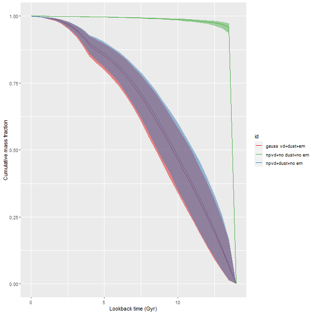
Here is the modeled mass growth history for a single spectrum of a region just south of the nucleus that had the largest difference in model SFH in the second set of runs, and the largest optical depth of attenuation in the first and 3rd. This is an extreme case of the shift towards older populations required by the neglect of reddening. Well over 90% of the present day stellar mass was, according to the model, formed in the first half Gyr after the big bang with almost immediate and complete quenching thereafter. While not an impossible star formation history it’s not one I often see result from these models, which strongly favor more gradual mass buildup.
NGC 4949 – modeled mass growth histories for models with and without an attenuation model
So, the conclusion for now is that having an attenuation model matters a lot, the detailed stellar kinematics not so much. Of course this is a relatively simple example because it’s a rapid rotator and the model convolution kernels are fairly symmetrical throughout the galaxy. The massive ellipticals and especially cD galaxies with more complex kinematics might provide some surprises.
Well that was simple enough. I made a simple indexing error in the R data preprocessing code that resulted in a one pixel offset between the template and galaxy spectra, which effectively resulted in shifting the elements of the convolution kernel by one bin. I had wanted to look at a rotating galaxy to perform some diagnostic tests, but once I figured out my error this turned out to be a pretty good validation exercise. So I decided to make a new post. The galaxy I’m looking at is NGC 4949, another member of the sample of passively evolving Coma cluster galaxies of Smith et al. It appears to me to be an S0 and is a rapid rotator:
NGC 4949 – SDSS imageNGC 4949 – radial velocity map
These projected velocities are computed as part of my normal workflow. I may in a future post explain in more detail how they’re derived, but basically they are calculated by finding the best redshift offset from the system redshift (taken from the NSA catalog which is usually the SDSS spectroscopic redshift) to match the features of a linear combination of empirically derived eigenspectra to the given galaxy spectrum.
First exercise: find the line of sight velocity distribution after adjusting to the rest frame in each spectrum. This was the originally intended use of these models. This galaxy has fairly low velocity dispersion of ~100 km/sec. so I used a convolution kernel size of just 11 elements with 6 eigenspectra in each fit. Here is a summary of the LOSVD distribution for the central spectrum. This is much better. The kernel estimates are symmetrical and peak on average at the central element. The mean velocity offset is ≈ 9.5 km/sec, which is much closer to 0 than in the previous runs. I will look briefly at velocity dispersions at the end of the post: this one is actually quite close to the one I estimate with a single component gaussian fit (116 km/sec vs 110).
Estimated LOSVD of central spectrum of NGC 4949
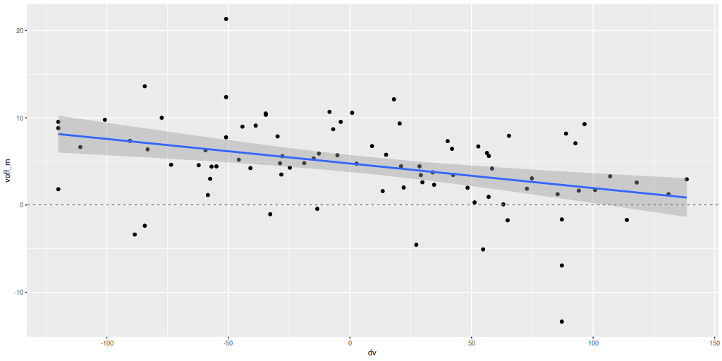
Next, here are the posterior mean velocity offsets for all 86 spectra in the Voronoi binned data, plotted against the peculiar velocity calculated as outlined above. The overall average of the mean velocity offsets is 4.6 km/sec. The reason for the apparent tilt in the relationship still needs investigation.
Mean velocity offset vs. peculiar velocity. All NGC 4949 spectra.
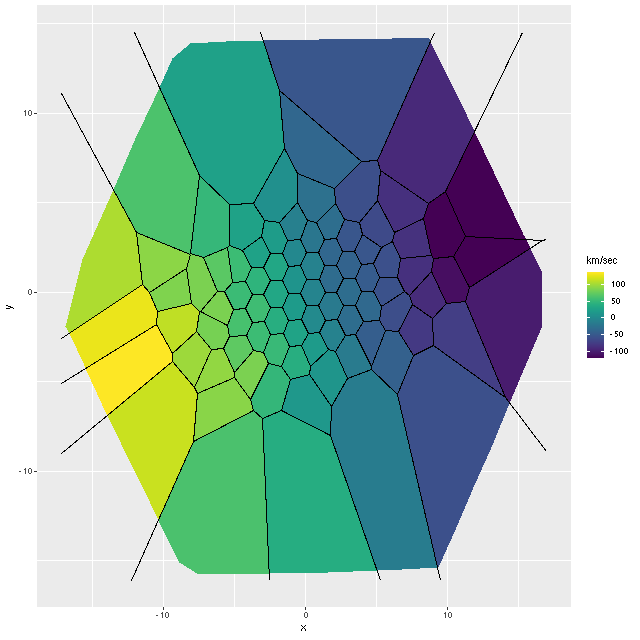
Exercise 2: calculate the LOSVD with wavelengths adjusted to the overall system redshift as taken from the NSA catalog, that is no adjustment is made for peculiar redshifts due to rotation. For this exercise I increased the kernel size to 17 elements. This is actually a little more than needed since the projected rotation velocities range over ≈ ± 100 km/sec. First, here is the radial velocity map:
Radial velocity map from Bayesian LOSVD model with no peculiar redshifts assigned.
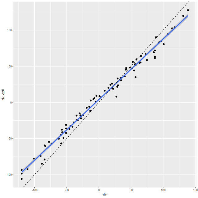
Here’s a scatterplot of the velocity offsets against peculiar velocities from my normal workflow. Again there’s a slight tilt away from a slope of 1 evident. The residual standard error around the simple regression line is 6.4 km/sec and the intercept is 4 km/sec, which are consistent with the results from the first set of LOSVD models.
Velocity offsets from Bayesian LOSVD models vs. peculiar velocities
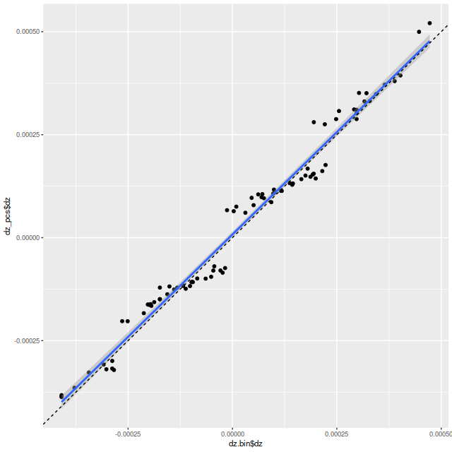
Exercise 3: calculate redshift offsets using a set of (for this exercise, 6) eigenspectra from the SSP templates. Here is a scatterplot of the results plotted against the redshift offsets from my usual empirically derived eigenspectra. Why the odd little jumps? I’m not completely sure, but my current code does an initial grid search to try to isolate the global maximum likelihood, which is then found with a general purpose nonlinear minimizer. The default grid size is 10-4, about the size of the gaps. Perhaps it’s time to revisit my search strategy.
Redshift offsets from a set of SSP derived eigenspectra vs. the same routine using my usual set of empirically derived eigenspectra.
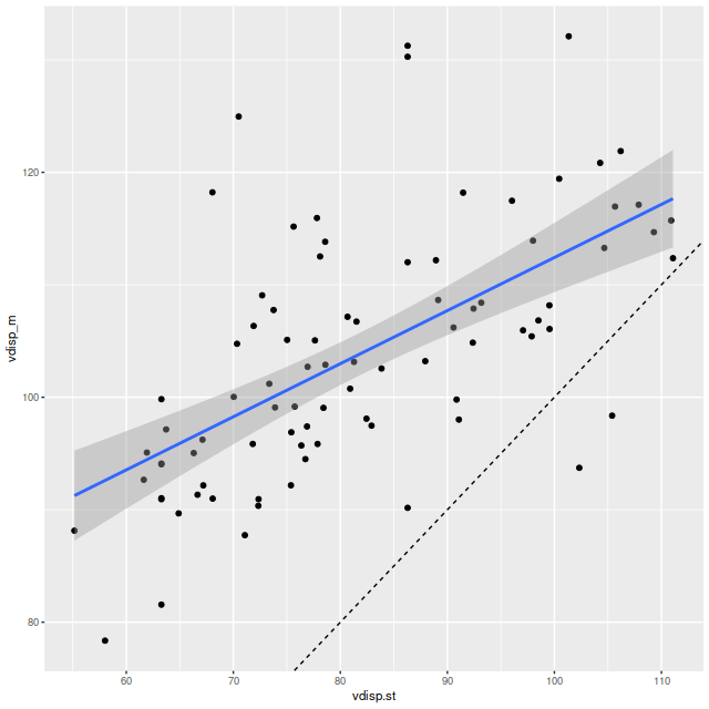
Final topic for now: I mentioned in the last post that posterior velocity dispersions (measured by the standard deviation of the LOSVD) were only weakly correlated with the stellar velocity dispersions that I calculate as part of my standard workflow. With the correction to my code the correlation while still weak has greatly improved, but the dispersions are generally higher:
Velocity dispersion form Bayesian LOSVD models vs. stellar velocity dispersion from maximum likelihood fits.
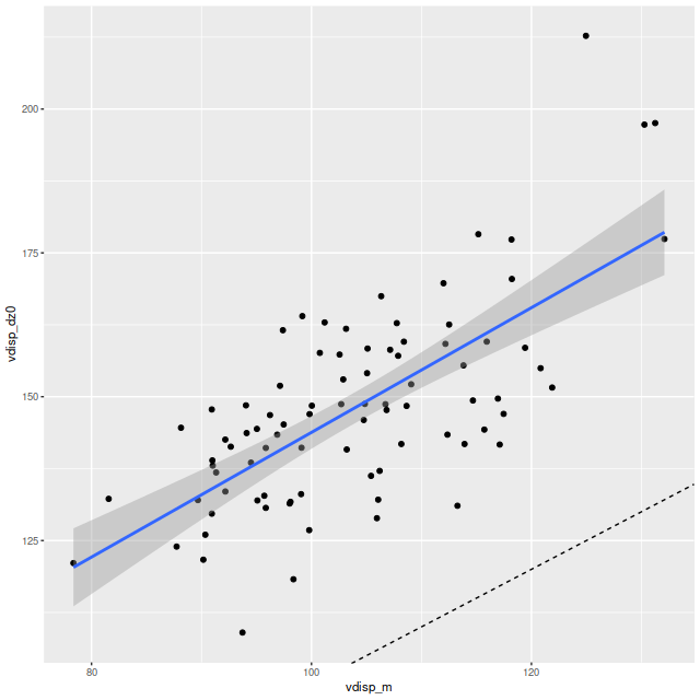
A similar trend is seen when I plot the velocity dispersions from the LOSVD models with correction only for the system redshift and a wider convolution kernel (exercise 2 above) with the fully corrected model runs (exercise 1):
These results hint that the diffuse prior on the convolution kernel is responsible for the different results. As part of the maximum likelihood fitting process I estimate the standard deviation of the stellar velocity distribution assuming it to be a single component gaussian. While the distribution of kernel values in the first graph look pretty symmetrical the tails are on average heavier than a gaussian. This can be seen too in the LOSVD models with the larger convolution kernel of exercise 2. The tails have non-negligible values all the way out to the ends:
Now, what I’m really interested in are model star formation histories. I’ve been using pre-convolved SSP model templates from the beginning along with phony emission line spectra with gaussian profiles with some apparent success. My plan right now is to continue that program with these non-parametric LOSVD’s. The convolutions could be carried out with posterior means of the kernel values or by drawing samples. Repeated runs could be used to estimate how much variation is affected by uncertainty in the kernel.
How to handle emission lines is another problem. For now stepping back to a simpler model (no emission, no dust) would be reasonable for this Coma sample.
This paper by J. Falcón-Barroso and M. Martig that showed up on arxiv back in November interested me for a couple reasons. First, this was one of the first research papers I’ve seen to make use of the Stan language or indeed any implementation of Hamiltonian Monte Carlo. What was even more interesting was they were doing exactly something I experimented with a few years ago, namely estimating the elements of convolution kernels for non-parametric description of galaxy stellar kinematics. And in fact their Stan code posted on github has comment lines linking to a thread on discourse.mc-stan.org I initiated where I asked about doing discrete convolution by direct multiplication and summation.
The idea I was pursuing at the time was to use sets of eigenspectra from a principal components decomposition of SSP model spectra as the bases for fitting convolved model spectra, with the expectation being that considerable dimensionality reduction could be achieved by using just the leading PC’s, which would in turn speed up model fitting. In fact this was certainly the case, although at the time I perhaps overestimated the number of components needed 1I mentioned in that thread that by one criterion — now forgotten — I would need 42, which is about an 80% reduction from the 216 spectra in the EMILES subset I use but still more than I expected. and I found the execution time to be disappointingly large. Another thing I had in mind was that I wanted to constrain emission line kinematics as well, and I couldn’t quite see how to do that in the same modeling framework. So, I soon turned away from this approach and instead tried to constrain both kinematics and star formation histories using the full SSP library and what I dubbed a partially parametric approach to kinematic modeling, using a convolution kernel for the stellar component and Gauss-Hermite polynomials for emission lines. This works, more or less, but it’s prohibitively computationally intensive, taking an order of magnitude or more longer to run than the models with preconvolved spectral templates. Consequently I’ve run this model fewer than a handful of times and only on a small number of spectra with complicated kinematics.
Falcón-Barroso and Martig started with exactly the same idea that I was pursuing of radically reducing the dimensionality of input spectral templates through the use of principal components. They added a few refinements to their models. They include additive Legendre polynomials in their spectral fits, and they also “regularize” the convolution kernels with informative priors of various kinds. Adding polynomials is fairly common in the spectrum fitting industry, although I haven’t tried it myself. There is only a short segment in the red that is sometimes poorly fit with the EMILES library, and that would seem to be difficult to correct with low order polynomials. What does affect the continuum over the entire wavelength range and could potentially cause a severe template matching issue is dust reddening, and this would seem to be more suitable for correction with multiplicative polynomials or simply with the modified Calzetti relation that I’ve been using for some time.
I’m also a little ambivalent about regularizing the convolution kernel. I’m mostly interested in the kinematics for the sake of matching the effective SSP model spectral resolution to that of the spectra being modeled for star formation histores, and not so much in the kinematics as such.
I decided to take another look at my old code, which somewhat to my surprise I couldn’t find stored locally. Fortunately I had posted the complete code on that discourse.mc-stan thread, so I just copied it from there and made a few small modifications. I want to keep things simple for now, so I did not add any polynomial or attenuation corrections and I am not trying to model emission lines. I also didn’t incorporate priors to regularize the elements of the convolution kernel. Without an explicit prior there will be an implicit one of a maximally diffuse dirichlet. I happen to have a sample of MaNGA spectra that are well suited for a simple kinematic analysis — 33 Coma cluster galaxies from a sample of Smith, Lucey, and Carter (2012) that were selected to be passively evolving based on weak Hα emission, which virtually guarantees overall weak emission. Passively evolving early type galaxies also tend to be nearly dust free, making it reasonable not to model it.
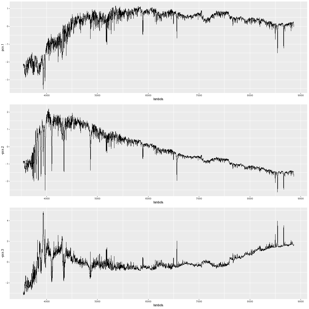
I’ve already run SFH models for all of these galaxies, so for each spectrum in a galaxy I adjust the wavelengths to rest frame using the system redshift and redshift offsets that were calculated in the previous round. I then regrid the SSP library (as usual the 216 component EMILES subset) templates to the galaxy rest frame and extract the region where there is coverage of both the galaxy spectrum and the templates. I then standardize the spectra (that is subtract the means and divide by the standard deviations) and calculate the principal components using R’s svd() function. I again rescale the eigenvectors to unit variance and select the number I want to use in the models. I initially did this by choosing a threshold for the cumulative sum of the eigenvalues as a fraction of the sum of all. I think instead I should use the square of the eigenvalues since that will make the choice based on the fraction of variance in the selected eigenvectors. With the former criterion a threshold of 0.95 will result in selecting 8 eigenspectra, 0.975 results in 13 (perhaps ± 1). In fact as few as 2 or 3 might be adequate as noted by Falcón-Barroso and Martig. The picture below of three eigenspectra from one model run illustrates why. The first two look remarkably like real galaxy spectra, with the first looking like that of an old passively evolving population, while the second has very prominent Balmer absorption lines and a bluer continuum characteristic of a younger population. After that the eigenspectra become increasingly un-spectrum like, although familiar features are still recognizable but often with sign flips.
First three eigenspectra from a principal components decomposition of an SSP model spectrum library
The number of elements in the convolution kernel is also chosen at run time. With logarithmic wavelength binning each wavelength bin has constant velocity width — for SDSS and MaNGA spectra of 69.1 km/sec. If a typical galaxy has velocity dispersion around 150 km/sec. and we want the kernel to be ≈ ±3 σ wide then we need 13 elements, which I chose as the default. Keep in mind that I’ve already estimated redshift offsets from the system value for each spectrum, so a priori I expected the mean velocity to be near 0. If peculiar velocities have to be estimated the convolution kernel would need to be much larger. Also in giant ellipticals and other fairly rare cases the velocity dispersion could be much larger as we’ll see below.
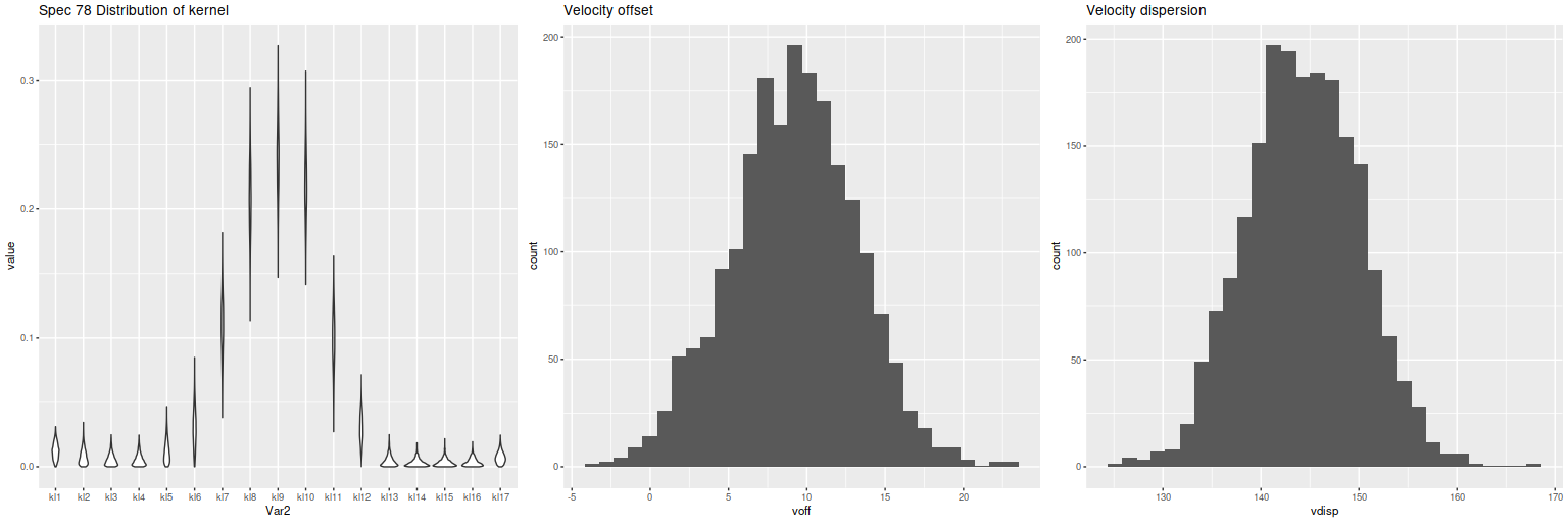
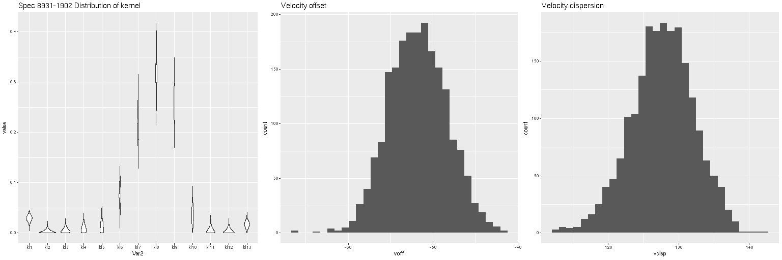
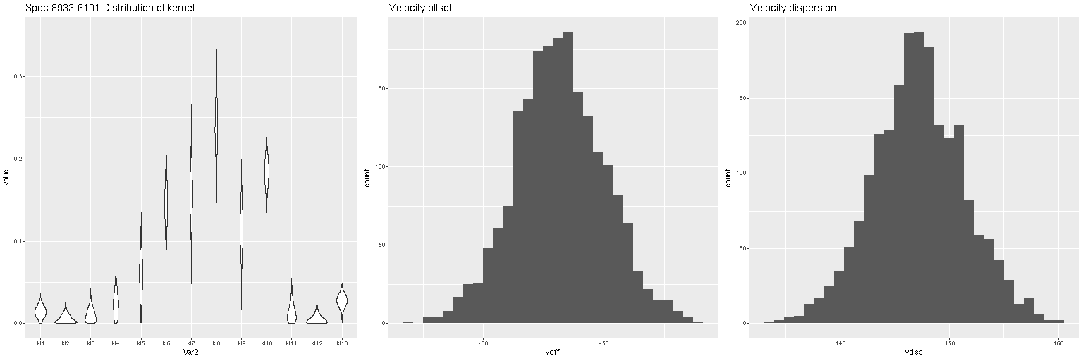
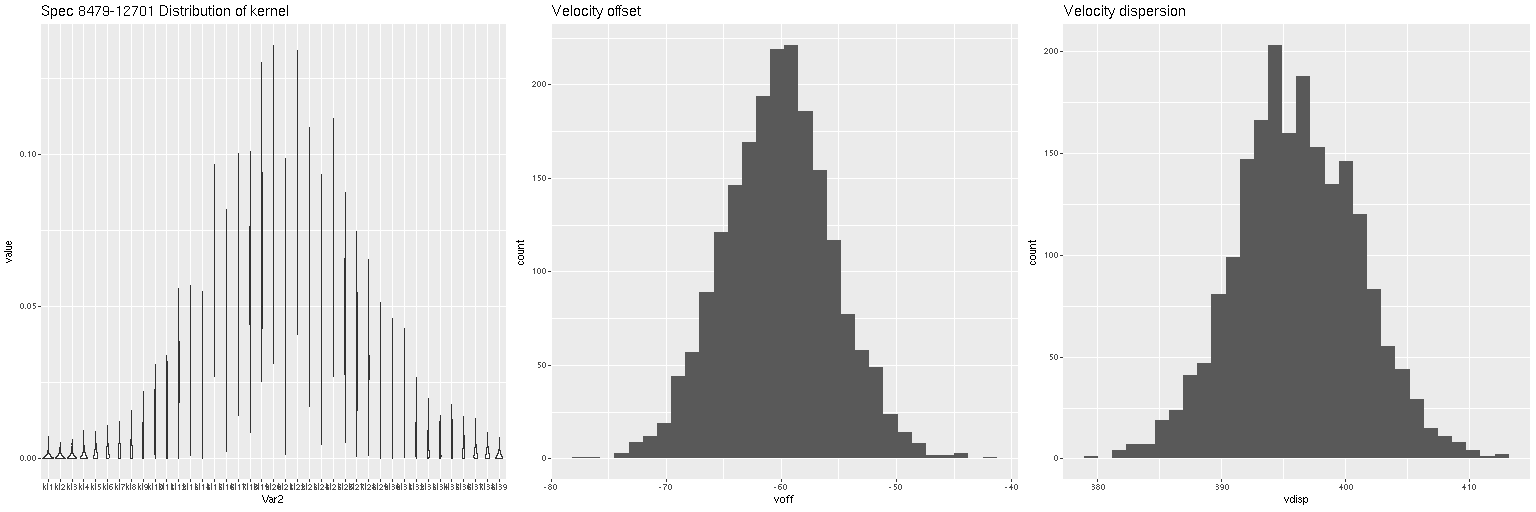
Lets look at a few examples. I’ve only run models so far for three galaxies with a total of 434 spectra. One of these (SDSS J125643.51+270205.1) appears disky and is a rapid rotator. The most interesting kinematically is NGC 4889, a cD galaxy at the center of the cluster. The third is SDSS J125831.59+274024.5, a fairly typical elliptical and slow rotator. These plots contain 3 panels. The left shows the marginal posterior distribution of the convolution kernels, displayed as “violin” plots. The second and third are histograms of the mean and standard deviation of the velocities. For now I’m just going to show results for the central spectrum in each galaxy. These are fairly representative although the distributions in each velocity bin get more diffuse farther out as the signal/noise of the spectra decrease. I set the kernel size to the default for the two lower mass galaxies. The cD has much higher velocity dispersion of as much as ~450 km/sec within the area of the IFU, so I selected a kernel size of 39 (± 1320 km/sec) for those model runs. The kernel appears to be fairly symmetrical for the rotating galaxy (top panes), while the two ellipticals show some evidence of multiple kinematic components. Whether these are real or statistical noise remains to be seen.
Distribution of kernel, velocity offset, and velocity dispersion. Central spectrum of MaNGA plateifu 8931-1902Distribution of kernel, velocity offset, and velocity dispersion. Central spectrum of MaNGA plateifu 8933-6101Distribution of kernel, velocity offset, and velocity dispersion. Central MaNGA spectrum of NGC 4889 (plateifu 8479-12701)
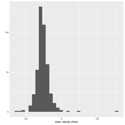
There are a couple surprises: the velocity dispersions summarized as the standard deviations of the weighted velocities are at best weakly correlated and generally larger than the values estimated in the preliminary fits that I perform as part of the SFH modeling process. More concerning perhaps is the mean velocity offset averages around -50 km/sec. This is fairly consistent across all three galaxies examined so far. Although this is less than one wavelength bin it is larger than the estimated uncertainties and therefore needs explanation.
Distribution of mean velocity offsets from estimated redshifts for 434 spectra in 3 MaNGA galaxies.
Some tasks ahead: Figure out this systematic. Look at regularization of the kernel. Run models for the remaining 30 galaxies in the sample. Look at the effect on SFH models.